EcosimPro Simulation of Transient Flow for Rocket Engine and Test Bench Applications

TABLE OF CONTENTS

ABSTRACT……….. 4

1. INTRODUCTION……… 6

2. ECOSIMPRO………... 7

2.1. Introduction……….... 7

2.2. ESPSS, European Space Propulsion System Simulation………... 8

2.2.1. General overview and key concept……… 8

2.2.2. Modelling………... 12

2.2.3. Libraries………. 13

3. FLUID TRANSIENT………... 23

3.1. Introduction……….... 23

3.2. Water hammer……… 23

3.2.1. Fluid transient flow concepts and basic differential water hammer equations……….. 23

3.2.2. Numerical solutions for 1D water hammer equations……… 42

3.3. EcosimPro modelling and validation work……… 48

4. TEST BENCH P2………. 52

4.1. Introduction……… 52

4.2. Test bench description………... 52

4.2.1. Lam1poldshausen Test Centre………... 52

4.2.2. P2: general overview……….. 53

4.2.3. Pressurization system………. 55

4.2.4. Propellant supply system……… 56

4.2.5. Purge system……….. 57

4.3. EcosimPro model………... 58

4.3.1. General overview………... 58

4.3.2. P2 components………... 61

4.3.3. Simulation input parameters ………. 69

4.3.4. Lines characteristics verifications……….. 76

5.1. Introduction……… 77

5.2. General overview………... 77

5.2.1. Ariane 5……….. 77

5.2.2. The upper stage engine: AESTUS………. 79

5.3. AESTUS EcosimPro model………... 82

5.3.1. General overview………... 82

5.3.2. AESTUS components on fuel side………. 83

5.3.3. AESTUS components: oxidizer side……….. 90

5.3.4. Simulation input parameters………... 94

6. MODEL VALIDATION……….. 97

6.1. Introduction……… 97

6.2. Test description……….…………. 97

6.3. Comparison with test results ……….……… 100

6.4. Sensitivity study………. 106

7. CONCLUSION………. 113

SYMBOLS……… 115

ABSTRACT

Storable propellant engine start-up is a complex phase which involves non-stationary hydraulic effects, two-phase flow. Each element of the engine, oxidizer and fuel lines, combustion chamber, has to be verified and qualified. For this purpose test facilities are an indispensable element for development and acceptance for space system, subsystem and components.

The partial failure of Ariane 5 flight No 510 on December 7 2001 called for the attention of liquid rocket propulsion engineers on the importance of the simulation of high frequency (HF) instabilities in propellant feed lines. The disturbances observed during the start-up of the flying engine were not triggered in any of the tests performed. As a consequence of the difference in the engine and test bench lines, transient phenomena result not predicable from a test campaign and so highly dangerous for engines performances and operation.

The knowledge of the flow characteristics in both the test benches and flying rocket stages is essential for future hardware design. Efforts have to be made for advancing the understanding of the transient flow behaviour in pipes for safe operation of the engine and for reducing the high costs and risks associated with tests. In this context, the development of tools for simulating the behaviour of flight-like feed systems by using non-flight-like test bench equipment are widespread.

In the present work a numerical investigation and evaluation of the critical fluid-system parameters is performed by means of the simulation and modeling software EcosimPro 4.4, based on C++ programming language. A hydraulic model of the test bench P2 in Lampoldhausen up to the test facility main valve is built up, as well as a simplified model of the Aestus engine. To validate and qualify the combined test bench-engine model, real on-ground test transients and steady-state results are compared with numerical results.

The numerical model has been successfully modified and adjusted and simulation results matched the measured values within acceptable ranges. Good agreement with steady-state-pressure, propellant mass flow rates behaviour and transient start-up in terms of water hammer peaks have been obtained. However, the water hammer frequencies have been not matched

accurately due to 1D-restrictions of the code and mainly to different characteristics of the simulated fluids.

Future efforts have to be done to improve the implementation of fluid property data bases implementation, especially for NTO (equilibrium condition between NO2 and N2O4 depending on

pressure and temperature) and for deeper understanding and investigation of possible influences of the content of pressurization gas content in the liquid fluid on the transient behaviour of the propellant feed system.

1.

INTRODUCTION

Numerical investigation and evaluation of steady-state and transient fluid system parameters is a key problem for the verification and qualification of stage element of the engine. Flow characteristics of both test benches and applied rocket stages is essential for future hardware design. Efforts have to be done for advancing the understanding of flow behaviour in pipe transient for the safe operation of the engine and to reduce the high costs and risks linked to a pure testing. Following this trend, propulsion system modelling and use of test data from computer simulation as calibration data are widespread.

In particular the partial failure of Ariane 5 flight 510 in 07 December 2001 has drawn attention to the importance of the real feed lines simulation in high frequency (HF) instabilities, phenomena not observed in any of the tests performed, as a consequence of the difference in the engine and test bench lines. Attention has to be turn in the case of flow transient studies to the coupling of these two elements and to the evaluation of any difference in hydraulic lines configuration of test bench and feed line systems of the real thruster, due to the strong dependence of these phenomena on systems geometry.

The purpose of the present work is then the development of a numerical tool to simulate flight-like feed system behaviour by using non-flight-flight-like test bench equipment. The numerical investigation would be used for the evaluation of critical fluid-system parameters. The physical modelling and simulation software chosen is EcosimPro 4.4.

The main steps followed in the present work are:

• The build-up of a hydraulic transient EcosimPro model of the P2 up to the test facility main valve

• The creation of a hydraulic transient EcosimPro simplified model of the Aestus engine for validation purposes

• The validation and qualification of the combined test bench-engine model by means of real on ground test results comparison

2.

ECOSIMPRO

2.1. Introduction

EcosimPro is a physical simulation modelling tool with an integrated visual environment that provides intuitive tools for simulating different kind of system.

The project developed by Empresarios Agrupados A.I.E initiated in the early ‘90s with funds from the European Space Agency (ESA) with the aim of creating simulation software to model Environmental Control and Life support System (ECLSS) for the European modulus (COLUMBUS) of the International Space Station (ISS) and for Hermes. The original objective was not to construct a generic tool but specific software for the ECLSS.

By now EcosimPro can be used to model a larger number of simple and complex physical systems. The software provides an object-oriented non casual approach towards creating reusable components libraries and powerful symbolic and numerical methods capable of processing complex systems represented by differential-algebraic equations (DAE) or ordinary-differential equations(ODE) and discrete events.

The multidisciplinary nature of this modelling tool led to its use in many other disciplines, including fluid mechanics, chemical processing, control, energy, propulsion and flight dynamics.

The EcosimPro general math capabilities are:

• Symbolic handling of equations (eg: derivation, etc.) • Robust solvers for non-linear and DAE systems

• Math wizards for: defining boundary conditions, solving algebraic loops, reducing high-index DAE problems

• Mathematical algorithms based on graph theory to minimize the number of unknown variables and equations

2.2. EPSS, European Space Propulsion System Simulation 2.2.1. General overview and key concept

The EPSS software provides a collection of standard databases for the propellant, pressuring gases and other fluid simulation as a collection of components and functions for the spacecraft and launch vehicle propulsion system simulation to be used for analysis of concept definition, mission analysis, impact studies, investigation of anomalies and optimization, testing and pressuring gas/propellant loading.

The object oriented tool, with the propulsion library for example, allows the user to draw, and design at the same time, the propulsion system with components of that specific library with tanks, lines, orifices, thrusters and tees and enables both steady state and transient study. The user enhances the design with components from the thermal library (heaters, thermal conductance, radiators), control library (analogue/digital devices), electrical library, etc, to represent a functional propulsion system, e.g. fluid properties, pipe networking, including multi-phase fluid flow, two-phase two fluids tanks, non-adiabatic combustion chambers, chemistry, turbomachinery, etc.

The main features of this software are:

• Conservation equations for liquid, gas and two-phase flow regimes implemented,

• Fluid phase automatically calculated and a homogenous equilibrium model for a real fluid under two phase conditions with or without a non condensable gas (so that absorption/desorption is not considered),

• Flow inertia, inversion and gravity forces and high speed phenomena present, • Concentrated and distributes load losses calculated,

• Heat transfer between fluid and the wall is modelled,

• Special components as check valve and pressure regulators available. The EPSS software is structured in different areas summarized as followed.

A set of fluid property functions for the propellants, pressuring gases and ground fluids allowing for the calculation of real properties of the typical working fluids in propulsion systems.

A set EcosimPro libraries including: 1D Fluid Flow Library (to simulate cold gas flow, liquid flow and homogeneous equilibrium tow-phase flow, two fluid flow), Combustion Library (for chemical equilibrium of an arbitrary mixture of chemicals in transient and non-adiabatic conditions so that vaporization and global reaction times can be considered), Chemical Library, Tank Library, Turbo-machinery Library.

Every physical system can be described by means of the fundamental concepts presented in the following lines.

Component: basic simulation unit generated by EcosimPro Language (EL) represented by means of

variables, differential-equations, topology and event- based behaviour, defined from a system library or by the user, containing a mathematical description of the real-world component. Two kinds of components are programmed: abstract and operational components. Abstract component describe some physical behaviour that does not represent a complete component, but that can be used as a base for others. These components contain the main formulation later used in the operational

components. Within the component optional blocks can be included:

• PORTS interface with the environment outside the component and must be a type already declared

• DATA known data items of the component

• DECLS declaration of the local variables to the experiment • OBJECTS the instances of classes used in this component

• TOPOLOGY aggregation of other components and their connections • INIT initialization of the component

• DISCRETE discrete behaviour of the component

• CONTINUOUS continuous behaviour of the component

• OBJECTS declaration of the external objects defined with classes • INIT initial value (i.e. starting value) assigned to the boundary variables

Port connection type: set of variables to be interchanged in connections in order to join together more

components to interface one or to shape a new one. The program in this sense is hierarchical: it allows creation of more complex components from other equipped with ports and to inherit behaviour from other components (tried and tested code from parent components can be reused).

Partition: associated mathematical model for the component defining the causality of the final

model. It is the intermediate step between the component and the experiment.

Experiment: representation of different simulation cases. It enables the definition of the initial

conditions and the boundary conditions of the mathematical model and the desired solution (transient or steady state). Within the experiment four optional blocks can be included:

• DECLS declaration of the local variables to the experiment. • OBJECTS declaration of the external objects defined with classes. • INIT initial value (i.e. starting value) assigned to the boundary variables.

• BODY block that contains the sequential instruction which defines the experiment.

Libraries: general classification by disciplines of all components.

The EL is the basic language used in EcosimPro. This language has been developed to be used in modelling combined continuous-discrete physical systems. It is based on continuous modelling concepts, developed in the 1970’s, and modern object-oriented techniques so that components can be inherited from one another and can be aggregated to create other more complex and modular components. EL allows mathematical modelling of complex structures by automatically solving systems of differential-algebraic equations, it can also generate reports, plots and other hard copies from within a classical sequential language and it has the ability to reuse C, FORTRAN and C++ classes.

Three different types of statements can be used in EL, depending on the context: sequential, continuous (the only one allowed in classical languages such as FORTRAN and C++) or discrete (only statements are allowed in event-oriented modelling).

• Sequential statements are used for initializations, functions and discrete event bodies which require a strict execution order. They are executed progressively and allow for the user to

control the flow of the program. They can be used in all sequential parts (BODY INIT). An example of these statements are WHILE, IF and FOR cycles.

• Continuous statements are used to express sets of differential-algebraic equations where the order in which they are written is important. They create the core where the continuous physical models are defined.

• Discrete statements are used to express events controlled by conditional statements which indicate when an event occurs. The basic statement is WHEN which declares an event by waiting for a condition to become true, at which point the associated code is executed.

The EL language creates the basic component and the Libraries are the mechanism used to organize design information and to provide other functionalities. A Library in EL is a set of items: components, port types, global variables, classes and functions which are related to the same area. They are the natural way to group components and functions.

After all the preliminary steps, the problem is formulated as a system of differential-algebraic equations (DAEs) written as follows:

( ) ( )

[

]

( )

EcosimPro has a robust DAE solver called DASSL. It is useful to solve two general classes of problems: the ones for which y′

( )

possible to solve y′

_{( )}

in (1) by a difference approximation and then to solve the resulting equation for the solution at the current time tN using Newton’s method. DASSL is not limited to approximate y′

( )

order approximation, but it can also approximate the derivate using the kth order finite difference,

where k is between 1 and 5. The order k and the time step are automatically chosen by this method at each step on the basis of the behaviour of the solution.

The iteration technique is a Newton-Raphson method, and the iteration matrix required in this case can be given as a Jacobian analytical subroutine or calculated as a Jacobian numerically using finite differences.

2.2.2. Modelling

The first step to create a model in EcosimPro is to create a Library by either using the EcosimPro Language (EL) or by reusing the already existing component and create the schematic that represent the physical system, combining together the different elements. The next step involves the generation of an associated mathematical model or partition, then creating an experiment for this partition. Finally, the simulation can start.

Create a library

Select one component from the Libraries and set the data

Create a new component

Code components, ports , etc, in EL language

Compile into a library

Generate a partition

Create an experiment

Run the simulation

Create a component graphically

2.2.3. Libraries

FLUID PROPERTIES LIBRARY

Getting appropriate fluid properties is a matter of vital importance and the Fluid Properties Library provides a large collection of functions returning the value of fluid properties (or the complete thermodynamic state) and introducing relevant parameters such as temperature, pressure, internal energy, density, etc. Most of the common fluids used for rockets are available.

Fluids in EcosimPro are supported in different categories:

• Perfect gas: temperature dependent only transport and heat capacity properties obtained from CEA coefficients.

• Simplified liquid: non pressure dependent properties.

• Real fluid: density, sound speed, specific heat interpolated in external tables as function of the temperature and pressure, considering liquid conditions such as superheated, supercritical or two-phase). The mixture of real fluid with non-condensable gas is also allowed and the homogenous equilibrium model is used to calculate the properties (quality, void fraction...) in case of two-phase flow.

For real fluids properties, data tables provided with EPSS have been generated using three different methods:

• Running the NIST program: pressure is used as a parameter and temperature as the first independent variable. The tables cover the liquid, vapour and super-critical zones and can guarantee continuity between two-phase flow, vapour, liquid and super critical state.

• Using an EXCEL tool for some fluids such as MMH, UDMH not available with NIST program. • The user can finally build his own property files.

The following methods are used for calculating fluid properties in the EXCEL tool. The density is calculated according to Peng-Robinson's state equation of state. The saturation pressure is assumed to be a polynomial or exponential adjustment of the temperature. The enthalpy and entropy properties are

based on the calculation of the non-ideal term _      −       ∂ ∂ p T T p V

to be added to the cp(T) polynomial

adjustment coefficient calculated at zero pressure (ideal gases) assuming:

3 2 DT CT BT R A C_V = − _g + + + (2.2)

The Peng-Robinson equation is badly adapted to the NTO properties because of the fluid reactivity and the variable concentration of nitrogen oxides that must be considered in the gas phase. For this fluid, the gas properties are calculated by means of CEA equilibrium properties. Liquid properties are calculated using specific correlation for a semi-perfect liquid. The liquid table will give good results when temperature is below critical, and will have large errors when the critical temperature is approached.

Two main problems are faced. The first one refers to the difficulty to find reliable correlation for all properties of liquid N2O4 (NTO), which is directly linked to experimental study. The second one

deals with the spontaneous decomposition that takes place as soon as N2O4 is in gaseous state

(dissociation in NO2 at ambient pressure and 400 K and a second dissociation at higher temperatures

creating NO and O2). Taking this phenomenon into account implies calculating the chemical

equilibrium at every pressure and temperature of interest in the vapour and supercritical phase. This is done using the CEA code where reaction contribution to cp and thermal conductivity are taken into

account.

For perfect gas the thermodynamic state, as a function of ρ-T, is based on the classical perfect gas state equation. The energy calculations are based on the computation of the specific heat at constant pressure for ideal gases, as a function of the temperature only, by means of polynomial expression:

4 7 3 6 2 5 4 3 1 2 2 1T a T a a T a T a T a T a R Cp + + + + + + = − − _(2.3)

The functions giving the viscosity and the thermal conductivity, when data is available, are also based on polynomial expressions. Otherwise they are estimated with different methods.

For simplified liquid density, speed of sound and specific heat values are based on the tables read from the property file and are interpolated as function of the temperature only. Once the properties have been interpolated, the equation of state can be applied assuming constant compressibility with pressure:





Viscosity and thermal conductivity are also interpolated from external data as a function of temperature:

Viscosity=ν (T)

Conductivity=λ (T)

In case of a perfect gas-real liquid mixture, the homogeneous equilibrium model (HEM) of the mixture is calculated. One fluid must be a real fluid or a simplified liquid, the other a perfect non-condensable gas (NCG). The hypotheses done with this model are:

• NCG forms a homogenous mixture at uniform temperature with the real fluid • NCG occupies the same volume as the Real Fluid according to Gibbs Dalton Law • If NCG is present the Real Fluid vapour is saturated (relative humidity=1)

• NCG is insoluble in the liquid phase of the Real Fluid.

The heat capacity, viscosity and thermal conductivity are calculated as a mixture of a liquid and composed gas (vapour and NCG) .The mixture properties are a result of the weighing of the pure fluid with the mass fraction:

Pliq Pgas mix P Pliq Pgas mix P Pliq Pgas mix P x x x x c x c x c λ λ λ µ µ µ ) 1 ( ) 1 ( ) 1 ( − + = − + = − + = (2.5)

where x_mix is the mixture quality defined as the mass ratio of gas (vapour+ NCG).

The gas mixture transport properties and speed of sound are calculated. In the same way the speed of sound is specifically approximated as an equivalent two-phase mixture, where the vapour phase is a mixture of NCG with 100% humidity.

FLUID FLOW 1D LIBRARY

This Library is the EcosimPro library for 1D transient simulations of two-fluid, two-phase system. The main features of this library are:

• Conservation equations for liquid, gas and two-phase flow regimes.

• Automatic calculation of fluid phase (homogenous equilibrium model used to calculate a real fluid under two phase conditions with or without NCG)

• Flow inertia, inversion and gravity forces and high speed phenomena. • Calculation of concentrated (valves) and distributed load (pipes) losses • Inclusion of heat transfer between fluid and the wall.

• Special components such as check valves and pressure regulators.

In ESPSS fluid networks every component is a resistive or a capacitive component.

The C (capacitive) elements integrate the mass and the energy equations: they receive the flow variables (volumetric, mass and entropy flow) and deliver the state variables (pressure, density, velocity, chemical composition and enthalpy). These elements simulate a volume with several fluid ports. Ports that belong to C elements have a small dot in the middle of the arrow and need to be initialized in a different way according to the option chosen.

The simplest component belonging to this group is Volume. It represents an adiabatic volume with a given number of fluid ports and contains:

Mass conservation equation:

∑

Non condensable mass fraction (x_nc) conservation equation:

∑

Energy equation: 2 / ) ( 2 v e E dt dV P Q mH V dt dE E dt dV VE dt d mix in j mix mix mix mix mix mix + = − + = + +ρ ρ

∑

where j is the number of ports.

From the thermal point of view, the term Q_in permits the heat exchange of heat through a thermal

port. The average velocity of the volume is required for the total energy conservation equations and for the evaluation of the friction forces and the wall heat transfer. For this calculation, volumes are considered to be made of two sides (1), (2), each one with a certain number of ports.

The average velocity is computed as follow:

A m m v jin in

ρ

where the total mass flow rate entering the volume from the side (1) is:

∑

from the side (2):

∑

This average velocity will be transmitted to the ports and the effective port velocity will be:

) cos( )

(j v α

v = (2.12)

where α is the port angle.

Instead of simply adiabatic constant volume, it is also possible to have more complicated components like Chamber and Cavity that are generic variable volumes which also take into account the possibility of sonic limitation. The critical mass flow models phenomena such as compressible and sub-cooled choking and it is calculated at each port as a function of pressure, density and speed of sound of the lumped volume.

)

(

)

(

j

g

z

z

p

=

−

∆

ρ

M (momentum) elements explicitly calculate the mass flow between C elements and work in the

opposite way as a C component.

The basic resistive component is the Junction. It represents a concentrated load loss with sonic loss limitation where no mass accumulation and enthalpy flow is assumed.

This element contains the momentum conservation equation that dynamically calculates the mass flow (per unit area):

up crit mix mix G G v P v P dt dG Lv G dt dA dt dG A I I ρ ζ ζ ρ ρ ) ( 0.5 ) 0.5( ) 5 . 0 ( ) )( ( 2 2 1 2 2 1 + − + − + = + + + (2.14)

where 1,2 indicate the inlet and the outlet port.

The mass flow rate G instead of m (=GA) is used for preventing a singularity in the system at the complete cross section closing (A=0).

The linearization of the quadratic term GG in the momentum equation, when G<GLAM,takes in

account that pressures losses are linear with laminar mass flow regimes.

The pressure drop coefficient will be automatically calculated from the orifice area and the adjacent connected flow areas assuming abrupt area changes as follows:

2 1 2 2 2 1 ) 1 ( ) 1 ( 5 . 0 002 . 0 ) 1 ( ) 1 ( 5 . 0 002 . 0 A A A A A A A A th th b th th f − + − + = − + − + = ζ ζ (2.15)

or can be an input of the user.

Valve and Filter components are built in the same way with a special arrangement of the momentum

equation.

ρ ρ µ µ n ref ref n ref ref m m P P P dt dm I I1+ 2) =( )1−( )2−∆ ( ) ( )2− ( (2.16)

where n is the exponent of the mass flow in the pressure loss equation.

For the Valve the derivative of the valve area in the momentum equation will be calculated as follows: tau A A dt dA _controlled − = (2.17)

Where A_controlledis the A0 s_pos.signal and tau is the time constant of area change (s).

The signal will be a boundary to be specified in the Experiment file or controlled by a component of the Control Library.

Pipe and Tube components are built as an alternation of Junctions and Volumes. They simulate a

cylindrical or rectangular area-varying non-uniform mesh 1D pipe or fluid vein.

The number of volumes in which the pipe is split into will be a parameter chosen by the user.

1D mass, energy and momentum equations, in transient regime, are incorporated so that all kind of flows (compressible or nearly incompressible flows, single or two components flow as well single or two-phase flow) can be simulated:

(2.18) ) ( ) ( ω ω ω Ω = ∂ ∂ + ∂ ∂ x f t

























=

E

v

nc

x

A

ρ

ρ

ρ

ρ

ω

_

In the first equation it must be noted that the source term responsible for the wall compressibility effect of the mixture, fundamental for the simulation of phenomenon like water hammer.

The equivalent distributed friction (∆ξ) calculates the pressure drop coefficient and the friction factor, including laminar and turbulent regimes.

At each discretized volume, the non-derivate state variables (pressure, qualities and temperature) will be calculated using the state function. If it is present a NCG, the homogenous equilibrium model will also be applied.

The sonic flow per unit area (ρu)crit is calculated at each pipe port as a function of the corresponding

node pressure, density and speed of sound. The last one will be used to take into account the sonic flow limitation

Models of arbitrary piping networks are built by an alternating C-M arrangement of the two types of Fluid Flow 1D component. Then a special component called Working Fluid defines the working fluid in a loop so that all interconnected elements will have the same fluids. For the first main fluid every category is possible, for the second fluid only perfect gases are allowed. Simplified liquids are supposed to have a zero constant vapour pressure, then, using this kind of fluid, bubble formation should take place when the pressure reaches a negative value. Pipe and Volume, so all the capacitive components will in this case calculate the corresponding void fraction and the pressure peaks due to bubble collapse.

It has to be noted that initializing a model and choosing the appropriate boundaries is an important point: boundary components will determine P, T, ρ and the mass fraction at the model interfaces. The simplest way to do this is using the component Vol_TM. It represents time dependent (TMD) boundary conditions and its purpose is to establish the complete thermodynamic state of a fluid port by imposing two variables (P-T, P-x, T-x..) and the non-condensable mass fraction(x_nc).

TANKS LIBRARY

Tanks play a fundamental role in rocket engine and spacecraft feed and pressurization system, an important role that can be evaluated using the Tank Library. This Library accounts for transient simulation of rocket engine and spacecraft tanks. Every component belonging to this Library can be

connected with the FLUID FLOW 1D component with the aim of simulating a complete rocket engine cycle.

The most important features are the following:

• Gas, liquid and two-phase regimes modelled for ideal and real fluids. Mixtures of real fluid (two phase condition) with or without NCG are included.

• Correlation to calculate the heat transfer between the tank walls and the fluid cavities • Bladder tank component, including bladder motion calculation is present.

• Single tanks 1D ,working with a pressuring gas and a liquid, are available including liquid level calculation (liquid and gas, heat exchange with the walls, mass and heat exchange at the liquid/gas interface).

This element allows for the calculation of the liquid level evolution assuming that the gas mixture (vapour plus NCG) is separated from the liquid and assuming liquid and gas phases at the same equilibrium temperature.

The mass, energy and momentum equations are basically the same present in the Pipe with additional moving grid terms corresponding to a variable volumes discretization:

i jun i i i jun i wall i jun i jun i i i i i i i i i fch i fch i dif i dif i jun i jun i i i i L A T T q mh mh V u V u u m m m m m m V V , 1 , , , 1 , , 1 , 1 , 1 , , 1 , ' ' ) / )( ( ) ( ) ( ' ) ' ' ( + + = − + + − − + − + − = + − − − − − − λ ρ ρ ρ ρ ρ (2.19)

The diffusive mass flow at the exit of volume i is calculated as follows:

i jun i i dif _L A m _, ( / )_1−1/2( )_{−1/2 ,} ∂ ∂ = µ ρ ρ (2.20)

The phase change (boiling or condensation) mass flow at the exit of the volume i is estimated as follows, when the temperature of the gas control volume is equal to or less than Tsat_gas:

) 1 ( , _

,i turb sat liqi i i fich f V x

m = ρ − (2.21)

when the temperature of the liquid control volume is greater than or equal to Tsat_liq ,the boiling of the

liquid volume is obtained as:

i i i vap sat turb i fich f V x m _, = ρ _{_ ,} ( ) (2.22)

The number of fluid (gas and liquid) and thermal nodes have to be taken equal to one, if it is not necessary to calculate the thermal stratification in the tank.

The temperature variations in the wall and in the liquid and gas sides, are calculated along the vertical axis. Heat transfer and mass transfer at the liquid/gas interface as well at the wall interface are also taken into account.

The use of special components like Sphere_ins and Cylinder_ins, connected to the respective thermal ports of the Tank, model the insulation layer according to its conductance properties.

Most typical wall shapes, to model heat conductivity in walls and insulations, are present.

The gravity is only in one direction, top or bottom and the lateral acceleration is not included in the calculation. The liquid height of the tank is taken into account to calculate the liquid column pressure.

Other fundamental libraries present in EcosimPro are:

• The Turbo Machinery Library for the simulation of pumps, turbines and compressors. • The Combustion Chamber Library for modelling of rocket engines

• The Control library that provides the custom items needed to represent analogue and digital control systems

• The Thermal library supplied with components to predict temperature distributions and heat flows in systems and devices using the thermal network method.

3. FLUID TRANSIENTS

3.1. Introduction

Flow in pipelines and channels are usually unsteady. A change from the steady state flow in a piping system occurs because of a change in boundary conditions.

There are many kinds of boundary conditions that may introduce transients. Common ones are changes in valves settings, starting and stopping of pumps, waves on a reservoir and unstable pump or fan characteristics. The changes in flow, acceleration and slow down of the fluid masses, can cause large pressure or depth fluctuations which can endanger the integrity of pipes. Such large fluctuations are the most dangerous events which the lines will be exposed to.

These pressure fluctuations are called pressure transients and the corresponding flow, transient

flow. To describe unsteady flow the word water hammer is used synonymously, although it is

customarily restricted to water.

Operation of spacecraft propulsion systems is regularly adversely faced with water hammer. The presence of very low pressure or vacuum conditions complicates the classically known water hammer, due to various phenomena such as cavitation, absorption and desorption of a pressurizing gas.

In the following chapter the water hammer phenomenon and the relevant factors influencing its behaviour are presented. In the last paragraph, an EcosimPro schematic for validation purposes is described.

3.2. Water hammer

3.2.1. Fluid transients flow concepts and basic differential water hammer equations

General overview

Water hammer mainly concerns with the generation, propagation and reflection of pressure waves in liquid filled pipe systems. Sudden shut-down of a pump or closure of a valve causes

formation, hydraulic and structural vibrations and excessive mass oscillation. Large pressure waves are transmitted through the system with the speed of sound, causing additional pressures in networks. These waves can have very steep front prone to excite the structural system.

In a solid body, a common practice for the analysis of a mass being acted on by a force is to consider the mass concentrated at its centroid. This technique can be applied to a mass of water as well. If the mass is very long and thin, as occurs in pipelines and channels, such an approach is not realistic. When a force is applied to a long mass, the force is propagated by wave action. The wave transmission takes a finite time interval and the entire mass involved does not experience the force at the same time.

An analysis that takes into account this phenomenon is called elastic analysis, whereas the method used for solid bodies is said to be a rigid body analysis. Thus the basic methods for the study of an unsteady flow are: the rigid column theory and elastic theory. In the former, the pipeline is considered rigid and does not deform under the pressure as well as the fluid, which is assumed to be incompressible. In the latter, both the elasticity of the fluid and of the pipe is taken into account.

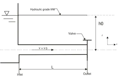
The simplest and most representative fluid transient case to consider is a sudden valve closure at the end of a pipeline. The mass of fluid that was moving forward with velocity v0 before the

closure, builds up a high pressure shock wave due to the sudden stoppage. The water downstream

the valve will attempt to continue flowing, creating a vacuum that may cause the pipe to collapse or implode. The more rapid the valve closure the more rapid is the change in momentum, hence greater is the additional pressure development.

Figure 3.1. - Reservoir-Pipe-Valve system.

The complete cycle that results from an instantaneous closure of a valve is briefly presented. At the instant the valve closes, the fluid nearest the valve is compressed, brought to rest and the pipe wall is stretched. The process is repeated for the next layer of fluid. The fluid upstream, from the valve continues to move downstream with the same speed v0 until the successive layers have been

compressed back to the source. The high pressure moves upstream as a wave, bringing the fluid to rest as it passes, compressing it and expanding the pipe. When the wave reaches the upstream end all the fluid is stopped and it is under the extra head h. All the momentum has been lost and the kinetic energy has been transformed into elastic energy.

Figure 3.2 - Propagation of pressure wave at t=ε v = v0 h0 h x z L

hydraulic grade line v = v0

h0

x z

L

Hydraulic grade line

Inlet Outlet

Figure 3.3 - Propagation of pressure wave at t=L/a

Since the reservoir pressure is unchanged, an unbalanced condition at the upstream end is present. The fluid starts to flow backward returning the pressure to initial value and the pipe wall in the initial configuration. Thus the flow proceeds at velocity v0 in the backward direction. The

unbalanced pressure energy is then converted into kinetic energy. This process of conversion travels downstream in the pipe with the speed of sound a. At the moment the wave arrives at the valve the pressure is again at the starting value and the velocity is everywhere v0.

Figure 3.4 - Propagation of pressure wave at t=L/a+ε v = 0 h0 h x z L

hydraulic grade line

h0 h

x z

L

hydraulic grade line

v = 0 v = -v0

Figure 3.5 - Propagation of pressure wave at t=2L/a

Since the valve is still closed, no fluid is available to maintain these conditions. A –h pressure head develops such that the fluid is brought to rest. This low pressure wave travels again backward and brings all of the fluid to rest, causing its expansion and the contraction of the pipe. At the moment the wave is again at the upstream end, the fluid is completely at rest and at the uniform pressure head –h with respect to the initial one.

Figure 3.6. - Propagation of pressure wave at t=2L/a+ ε v =- v0

h0

x z

L

hydraulic grade line

v =- v0

h0

x z

L

hydraulic grade line

v = 0

Figure 3.7 - Propagation of pressure wave at t=3L/a

Again an unbalanced condition is present at the reservoir. The fluid flows forward returning to normal conditions, as the wave progresses downstream at velocity a. At the instant the wave reaches the valve, the fluid conditions will be the same as at the initial time.

Figure 3.8 - Propagation of pressure wave at t=3L/a+ ε

h0

x z

L

hydraulic grade line

v = 0 h v = v0 h0 x z L

hydraulic grade line

v = 0

Figure 3.9 - Propagation of pressure wave at t=4L/a

This process will be repeated every 4L/a if the pipe is perfectly frictionless and no elastic structural interaction is considered. The half interval (2L/a) after which conditions are repeated, is termed the theoretical period of the pipeline.

In real systems the pressure waves are dissipated due to friction losses as the wave propagates in the pipeline, and the fluid becomes stationary after a short time.

The following characteristics may reduce or eliminate water hammer: • Low fluid velocities(flow velocity at or below 1.5 m/s for water) • Slowing closing valves

• High pipeline pressure rating • Water towers

• Air vessels • Surge tanks

To prevent this phenomena air vents or vacuum relief valves are installed. Shorter lengths of straight pipe with elbows are preferred to reduce the influence of pressure waves.

v = v0

h0

x z

L

Water hammer equations

All methods of analysis of unsteady flow in conduits starts with the equation of motion, continuity energy, plus equations of state and other physical property relationships.

Assuming that the fluid is under a pressure that increases along the pipe length L and that the diameter increases in the same direction of increasing x the following expression for the continuity equation is valid:

0 2 ₌ ∂ ∂ + ∂ ∂ + ∂ ∂ x v a x P v t P ρ (3.1)

The equation of motion, in terms of centreline pressure P(x, t) and average velocity v(x, t), states that the resultant x component of force in the control volume is equal to the time rate of increase of x momentum within the control volume plus the net efflux of momentum from the control volume: 0 2 ∂ = ∂ + ∂ ∂ + ∂ ∂ + + ∂ ∂ t v x v v x z g D v fv x P H ρ ρ ρ (3.2)

In most treatments the hydraulic grade h, and the discharge Q are preferred dependent variables, while x and t are the independent variables. Using these as variables, and assuming cavitation, leakage and blockage absent, the convective transport terms u

x h ∂ ∂ , v x v ∂ ∂ , u x z ∂ ∂

are very small compared to other terms and therefore neglected. These restrictions cause only 0.1% of errors in the normal engineering situation. The simplified unsteady pipe flow equations are obtained:

0 2 = ∂ ∂ + ∂ ∂ t Q gA a t h (3.3) 0 2 1 2 = + ∂ ∂ + ∂ ∂ gDA Q fQ t Q gA x h (3.4)

The Equations (3.3) and (3.4) are valid as long as the flow is 1D, the duct properties (diameter, wave speed, temperature) are constant and the friction force can be approximated by the Darcy-Weisbach formula for steady state flow. In addition it is always assumed that the friction factor f is either constant or weakly dependent on the Reynolds number.

In the hypothesis of a rigid column analysis, the pipeline is rigid. No useful information could be obtained from the continuity equation in this case. Integrating the momentum equation over a finite pipe line, it is possible to obtain the well-known Allievi-Joukowsky equation:

v g a

h=± ∆

∆ (3.5)

The pressure peak due to the sudden valve closure is a function of the dimensions of the pipe (diameter and length), speed of the fluid, its density and mostly of the closure time of the valve. The equation above also shows that over an increase in velocity at the gate, the head there must be reduced. So the minus sign has to be used for waves travelling upstream and plus for waves travelling downstream.

The range of validity of this expression is given by a valve closure time less than 2L/a. A valve closure can be approximated by a series of very small steps of closure spread over a period of time. Each step causes a ∆v decrement and a corresponding wave. If the last wave, created during the closure, is emitted before the first wave is reflected back, the sum of all the initial positive small waves will be equal to the corresponding wave produced by an instantaneous closure. On the other hand, if any wave has been reflected before the last wave is emitted, the resulting wave must be smaller than the wave emitted for a closure in less than the time of 2L/a. Thus, the magnitude of a wave generated by a rapid closure of a valve at the downstream end of a simple pipeline is equal to that of the wave produced by an instantaneous closure. If the closure takes more than 2L/a, the magnitude of the wave is smaller. For very long pipelines the value of the pipeline period (2L/a) can be very large. In this situation, what initially could be intended as a really slow rate of valve movement could result in a sudden closure with the consequent generation of large pressure oscillations. In the case of a network, it can be difficult to establish a value for the reflection time.

Transmitted and reflected pressure waves lead to one main oscillation flow in a pipe-line with a natural frequency of the pipe. The time period after which the natural frequency of water column gets stabilized depends on the elasticity of the pipe material.

Unfortunately water hammer is not only a pressure wave travelling in a liquid at the speed of sound. The conditions in pipeline systems can be far from the idealized situation described by the

classical water hammer theory. Possible sources that may affect the waveform are friction, cavitation and a number of fluid-structure interactions effects (FSI).

Speed of sound

The magnitude of pressure waves depends strongly on the speed of sound. The value of the acoustic velocity itself depends on the bulk modulus or compressibility of the fluid.

For rigid pipe walls, the velocity of water hammer waves in a compressible fluid can be calculated by:

ρ

K

a= (3.6)

The bulk modulus is affected by pressure, temperature and gas content of the liquid. The free gas, being highly compressible, increases the compressibility of the fluid. When small quantities of gas are available in the liquid, the elasticity tends to that of the gas whilst the density remains close to that for the liquid. The effect predicted from Equation (3.6) is to reduce the pressure wave velocity to well below that of either the liquid or the gas. Assuming homogeneous flow, the pressure wave velocity in a gas-liquid mixture at atmospheric pressure, can be evaluated substituting in the Equation (3.6) the following expressions for mixture bulk modulus:

)

1

(

1

+

−

=

K

K

V

V

K

K

So that the speed of sound assumes the following form:

) 1 ( 2 α α ρ ρ − = l g ga a (3.9)

One percent of gas by volume reduces the pressure wave velocity in water to 120 m/s compared to 1400 m/s without any gas. If it is relatively simple to calculate the wave speed given a particular percentage of bubble in the liquid, it is not so simple to determine how the bubble content varies with pressure and time. Solids in liquids have a similar but less drastic influence, unless they are compressible.

Not only the bulk modulus of the fluid affects the value of the speed of sound, but also the elastic properties of the duct, as well as the external constrains. Elastic properties include the duct size, wall thickness and wall material; the externals involve type of supports and freedom of movement in the longitudinal direction. To consider the influence of the elasticity of the pipe walls upon the propagating pressure wave, the bulk modulus needs amendment to take the deformation effects into account. Together with the Equation (3.6), derived for the rigid column theory, the water hammer wave velocity is modified in order to account for the bulk modulus reduction due to contraction and expansion of the pipe walls. The following general expression is presented by Halliwell for the wave velocity:

) 1 ( ψ ρ s D E K K a + = _(3.10)

in which ψ is a non dimensional parameter that depends upon the Poisson's ratio and the pipe restraint. For a thin-walled pipeline wave speed formulas are developed for different kind of support.

For a pipe anchored at its upstream end only:

) 4 5 ( 1 ( 1 µ ρ + − = sE D K a _(3.11)

For a pipe anchored throughout:

) 4 5 ( 1 ( 1 µ ρ + − = sE D K a _(3.12)

) 1 ( 1 sE D K a + = ρ (3.13)

The final expression taking into account gas compressibility and wall elasticity for the speed of sound is: ) 1 ( ) 1 ( 1 ref ref mix _K D_{sE p} a α ρ α + + − = _(3.14)

Where p_ref is the pressure and α_ref the void fraction at reference conditions.

Fluid-Structure Interaction (FSI)

The classical theory of water hammer predicts a squared-wave pressure history in a reservoir-pipeline-valve system subject to sudden valve closure. This square wave is distorted with the introduction of high-frequency pressure oscillations due to secondary effects. This can make the wave front less steeper, increase the system main frequency and invalidate the use of Joukowsky’s formula.

If non-zero dynamic stresses and strain in the pipe wall are taken into account the extended

theory of water hammer has to be considered.

The axial-radial vibration of liquid-filled pipes, excited by water hammer waves are described by the so-called four-equation model. It permits the coupled propagation for pressure waves in the liquid and axial stress waves in the pipe wall. The FSI coupling mechanism is often referred to as

Poisson’s coupling, because it is induced by radial/axial pipe contractions which are proportional

to Poisson’s ratio. Due to radial expansion of the pipe, induced by pressure rise in the fluid, axial contractions of the pipe are induced. These contractions send out stress waves and an associated pressure change in the fluid, called precursor waves. The precursor waves are stress-wave-induced disturbances in the liquid that travel ahead of the classical water hammer wave. The effects created are initially very small. However their cumulative effect can be significant.

0 1 = ∂ ∂ + ∂ ∂ fluid x P t v ρ (3.15) 0 2 ) 2 1 ( = ∂ ∂ − ∂ ∂ + + ∂ ∂ x E t P Es R K x v µ σx _(3.16) 0 1 = ∂ ∂ − ∂ ∂ x x u _x str x σ ρ & (3.17) 0 1 = ∂ ∂ − ∂ ∂ − ∂ ∂ t P Es R t E x u&_x σ_x µ _(3.18)

The model is valid for the low-frequency acoustic behaviour of straight thin-walled, linearly elastic, liquid-filled, prismatic pipes of circular cross-section.

Writing the structural equation for axial motion, it can be immediately realized that this equation is coupled via σx, P and µ, representing the boundary conditions that account for the contact

between liquid and pipe wall on the interface, with the mass conservation equation. This is what will be referred to as Poisson's coupling. If the ratio s/R of wall-thickness to pipe-radius is then small with respect to unity, circumferential stresses are uniform in the wall cross-section and radial stresses are neglected. If this is not true axial/radial vibration of thick-walled pipes have to be considered and a correction of the FSI model is necessary.

Local FSI can also occur at valves, orifices, expansions, contractions, elbows, bends and branches. The dynamic interaction of a local component with fluid unsteadiness is called junction

coupling. Steep pressure wave fronts passing unstrained pipe bends will make the bends move.

The bend movements provide elastic storage capability for the contained liquid, which will affect the passing pressure waves. The “breathing” of the pipes provides a secondary elastic storage capability which also affects the pressure waves.

Another important phenomenon that has to be considered is the so-called friction coupling. It represents the mutual friction between liquid and pipe and, as the Poisson’s coupling, it acts along the entire duct length. In the previous treatment the friction has been neglected, so the initial head everywhere was assumed equal to the reservoir head h0. With friction, the steady state

situation is different. When the disturbance is introduced in the system, a pressure wave starts travelling in the pipeline. As the wave travels upstream, it produces a velocity reduction in layers

of fluid which are at progressively higher initial pressures, owing to friction presence. Then, considering a travelling wave, it is possible to see on the downstream side of the wave a pressure increase transmitted throughout a fluid already at high pressure. The pressure at the valve therefore rises higher and higher as the wave continues its progress in the pipe. This phenomenon is called line pack and takes a time equal to L/a to be transmitted to the valve. The continuous rise in pressure causes the fluid to compress further. The velocity just downstream of the wave is no longer zero as flow has to continue to supply fluid to fill the additional volume made available by this compression. The velocity difference hence diminishes and so also the wave magnitude is lower. This process is called attenuation and it is the process that attenuates the waves, finally extinguishing them. The wave shape is also modified by the line pack.

Figure 3.10- Line pack and attenuation [1]

Also, the material response is important for the water hammer phenomena behaviour. The visco-elastic behaviour of plastic pipes influences water hammer events, attenuating pressure fluctuations and increasing the dispersion of water hammer waves.

Column Separation

Concerning liquid transients in a pipeline system, there are two different types of flow regimes to analyse. The first is referred to as the water hammer regime or no cavitation case, where the pressure is above the vapour pressure of the liquid. The second is the cavitation regime, where the pressure is below the vapour pressure of the liquid. The magnitude of the absolute negative pressure in the system is governed by the flow conditions and the cavitation properties of liquid and pipe walls. Even if the pipe is really simple, additional complications arise if cavitation occurs. This phenomenon is of particular concern because of the strong impulsive load on the structure due to the violent cavity collapse, with consequent severe structural damage.

Two types of cavitation in pipelines can be distinguished depending on the void fraction α (ratio of the volume of vapour to the liquid/vapour mixture volume).

The first is the discrete vapour cavity or liquid column separation. This phenomenon refers to the breaking of a column in fully filled pipelines. It implies a large value of α and it is assumed to have a local character.

The column separation may occur in fluid transients having high peaks, or in systems in which transients are produced rapidly where the pressure may be reduced to the vapour pressure of the liquid at a specific location. The reduction in pressure causes a negative wave pulse to travel down the pipe reducing the velocity. The difference in velocity between portions of pipe flow tends to put the liquid column into tension, which commercial fluid can not stand. When the vapour pressure is reached a vapour cavity forms into the pipe. The vapour cavity, driven by the inertia of the parting fluid columns, starts growing. The size of this cavity increases until the difference between its internal pressure and the decreasing external pressure is sufficient to offset the surface tension. Once this critical size is reached, the vapour-filled cavity becomes unstable and expands explosively. Depending upon the system geometry and the velocity gradient, the cavity may become so large to fill the entire cross section of the pipe thus divide the liquid in two columns as in the specific case of column separation. This usually occurs in vertical pipes and pipes having steep slopes or sharp edges. The cavity acts like a vacuum retarding the columns, causing a significant increase in the wave reflection time. Such a lengthening for the pipe period (2L/a) is characteristic of the presence of separation. The cavity will diminish in size only when

partial pressures of the liquid vapours and the released gases. If the temperature of the liquid vapours is constant then the partial pressure of the liquid is constant. However the partial pressure of the gas can increase or decrease if the molar fraction in the cavity increases or decreases. If a cavity forms and collapses several times during a transient, the cavity increases in size with successive cavity formations. The following graph shows the typical pressure signature of a fluid transient in a pipeline modified by the presence of separation.

Figure 3.11- Pressure diagram for a pipeline where separation is occurring[13]

The latter cavity flow regime is the distributed vaporous cavitation or two-phase (bubbly) flow. It implies a small value of α. It is more common in case of horizontal pipes or pipes having mild slopes. The vaporous cavitation consists of a region of two-phase flow of both vapour and liquid appearing over an extended length of the pipe with the pressure at the liquid vapour pressure. If the liquid in the pipelines contains dissolved air or gases, a reduction below the saturation pressure causes gas bubble formation at the many nuclei generally present in technical liquids. These small bubbles greatly decrease the wave speed. If the temperature increases but the pressure is kept constant then the cavitation hammer decreases due to the decreased speed of sound in liquid and saturation pressure increase.

The collision of two columns or of one column with a closed end, or simply the cavities collapsing may cause a large and nearly instantaneous rise in pressure. A severe hydraulic load for the whole system is created. The duration of the pressure pulse is about one tenth of a 2L/a period and, if the difference in velocity between the columns at the moment of collapse of the cavity is ∆v, a head increase of a∆v/2g may be expected. The head directly caused by the cavity collapse is less than the water hammer head generated at the beginning, but a narrow short-duration pulse occurs. The resulting maximum head in the system could be greater than the maximum head predicted by Joukowsky equation, if the cavity collapse occurs exactly at the arrival of a pressure wave front. This head increase may be sufficient for the pipe to rupture. The maximum pressure head due to the collapse of a cavity in a simple valve-pipe-reservoir system is given by: v r f h v g a h_max = +2 ₋ (3.19)

where v_f is the velocity of the liquid column at the valve just before cavity collapse and hr−v is

the difference in elevation between the downstream valve and the upstream reservoir pressure head.

The location and intensity of column separation is influenced by several system parameters including the cause of the transient regime (rapid valve-closure, pump failure, turbine load-rejection), layout of the pumping system (pipeline dimensions, longitudinal profile and position of the valves) and hydraulic characteristics (steady flow-velocity, static pressure-head, skin

friction, cavitation properties of the liquid and pipe walls). Therefore it is very hard to judge the severity of the pressure peak following cavity collapse that may or may not exceed the Joukowsky’s pressure rise and cavities may form at the valve or/and along the pipe.

The situation can even be worse: the occurrence of water column separation can trigger a series of cavity formations and collapses resulting in a series of impulsive loads on the structure. The first cavity is often a single coherent void this will shatter into a cloud of smaller bubbles as a result of the violence of the first collapse. The cavities will grow and diminish according to the dynamic pressure of the system.

Figure 3.13 - Wave speed against fractional volume of gas for a water-air mixture[14]

Because of the presence of the bubbles, the liquid in a cavitating flow is a mixture of the released gases and the liquid. Experimental investigations have shown that there is more dissipation of the pressure waves in a gas-liquid mixture than in a pure liquid. The additional dissipation is due to the heat transfer to the liquid when the bubbles are expanded and compressed. To compute the energy dissipation in cavitating flows, the total shear stress is determined by adding to wall shear stress, the shear stress due to non-adiabatic behaviour of a spherical bubble:

v L v h gD C _l bubble = α ρ ∆ τ 0 (3.20)

where C is an unknown constant and α0 the void fraction at the reservoir pressure.

Accompanying the generation of vapour there is also a release of gas from solution in the liquid. At atmospheric pressure in a liquid there will commonly be a content of free bubbles. When the pressure changes the bubble content will change. Due to pressure drops caused by the water hammer phenomenon, there will be an increase in volume of bubbles present. This change in volume can be really large if the drop in pressure is great. A very small amount of gas comes out when the pressure is below atmospheric pressure, but progressively more and more comes out as the pressure drops further. If the diffusion of gas in the fluid towards bubbles is a relatively slow process, only small quantities of gas evolve during most transients and the concentration of dissolved gas changes only slightly. However, due to the strong relationship between free gas void fraction, pressure and wave propagation speed, even a small quantity of free gas can have a profound influence on the behaviour of low pressure transient waves. For gas to come out of solution sufficiently rapidly, on the order of pressure transient, it is necessary for the pressure to drop sufficiently below a certain value, the so called gas head.

The presence of free gas does not significantly affect the formation of the separation bubble but it is considered to have a cushioning effect upon its closure. This is due to the fact that the solution for gas bubbles is slower than their evolution, so that the gas bubbles are left floating in the liquid after the main vapour-filled cavities collapsed. Thus they are available to reduce the magnitude of the pressure waves that would have been generated, decreasing the effective bulk modulus of the fluid.

Summarizing, a system in which cavitating flow and column separation occur can be divided in three regions: (1) water hammer (2) cavitation (3) column separation.

In the water hammer region, the void fraction is so small that it can be neglected, hence the velocity of the pressure waves does not depend upon pressure. In the cavitating region, gas bubbles are dispersed throughout the liquid and the fluid behaves like a gas-liquid mixture. In such flow the speed of sound depends upon the void fraction, which depends on the pressure. The classical water hammer equations are not valid in cavitating regions. The third region may be