Forward implied volatility expansions in LSV models

(1)

facoltà di scienze matematiche, fisiche e naturali

Corso di Laurea Magistrale in Matematica

Forward Implied Volatility Expansions

in LSV models

Tesi di Laurea in Matematica Finanziaria

Relatore

Presentato da:

Chiar.mo Prof.

Paolo Martini

Andrea Pascucci

II Sessione

(2)

(3)

Forward Implied Volatility

Expansions in LSV models

(4)

(5)

Ai miei genitori

Alla mia pulce Fabiana

(6)

(7)

Introduction

In this work we address the problem of finding formulas for efficient and

reliable analytical approximation for the calculation of forward implied volatility

in LSV models, a problem which is reduced to the calculation of option prices as

an expansion of the price of the same financial asset in a Black-Scholes dynamic.

The motivation for this work comes from financial mathematics, where the

prices of financial derivatives is reduced to the calculation of these expectations.

The speed of calculation of rates and calibration procedures is a very strong

operational constraint and we provide real-time tools (or at least more competitive

than Monte Carlo simulations, in the case of multi-dimensional diffusion) to meet

these needs.

Our approach involves an expansion of the differential operator, whose solution

represents the price in local stochastic volatility dynamics. Further calculations

then allow to obtain an expansion of the implied volatility without the aid of any

special function or expensive from the computational point of view, in order to

obtain explicit formulas fast to calculate but also as accurate as possible.

In the first chapter we introduce briefly the dynamics of black-schole and the

problem of implied volatility, explaining the importance of this value, but also the

difficulty of building models that are able to effectively simulate the behavior of

financial securities, and that provide implied volatility surfaces that are close to

the empirical data.

The second chapter of the thesis focuses on the work of Lorig, Pagliarini and

Pascucci, while in the third chapter we try to implement codes that allow to verify

the consistency of this method, but also to numerically analyze what are the most

convenient choices for a practical use of these formulas.

Finally, in the fourth chapter we attempt to extend this approach to the case of

forward implied volatility, performing some numerical tests on the Heston model.

(12)

(13)

C H A P T E R

1

B&S Model and IV problem

1 The Black&Scholes Model

In the early 1970s, Fischer Black, Myron Scholes, and Robert Merton achieved

a major breakthrough in the pricing of stock options ([BS73] and [Mer73]). This

involved the development of what has become known as the Black&Scholes (or

Black-Scholes-Merton) model. This model has had a huge influence on the way

that traders price and hedge options. It has also been pivotal to the growth and

success of financial engineering in the last 30 years.

1.1 Lognormal Property of Stock Prices

The model of stock price behaviour used by Black, Scholes and Merton is a

model which assumes that percentage changes in the stock price S in a short

period of time are normally distributed; given:

m: Expected return on stock per year

s: Volatility of the stock price per year

The mean of the return in a period of time Dt is m Dt, and the standard deviation of

the return is s

Dt , so that

(1.1)

DS

S

~

N

_{m Dt , s}

2

_Dt

where DS is the change in the stock price S in time Dt, and

N

m,v

denotes a normal

distribution with mean m and variance v. Formula (1.1) implies that:

(1.2)

ln

HS

T

L - lnHS

t

0

L~N

Jm+

s2 2

N HT-t

0

L , s

2

HT-t

0

L

and

(1.3)

ln

HS

T

L~N

ln

HS

t0

L+Jm+

s2 2

N HT-t

0

L , s

2

HT-t

0

L

where S

T

is the stock price at the future time T , while S

t

0

is the present stock price

(at time t

0 ). Formula (1.3) shows tha ln

HS

T

L is normally distribuited, so that S

T

has

a lognormal distribution. The mean of ln

HS

T

L is lnHS

t

0

L + Im - s

2 ‘ 2M HT - t

0 L and

the standard deviation is s

2 HT - t

0 L ; thus from (1.3) and the properties of the

(14)

(at time t

0 ). Formula (1.3) shows tha ln

HS

T

L is normally distribuited, so that S

T

has

a lognormal distribution. The mean of ln

HS

T

L is lnHS

t

0

L + Im - s

2 ‘ 2M HT - t

0 L and

the standard deviation is s

2 HT - t

0 L ; thus from (1.3) and the properties of the

lognormal distribution we have this equation for the expected value of S

T

:

(1.4)

E

PS

T

T = S

t

0

ã

m

HT-t

0

L

1.2 Black-Scholes-Merton differential equations

The Black-Scholes-Merton differential equation is an equation that must be

satisfied by the price of any derivative dependent on a non-dividend-paying stock.

They involve setting up a riskless portfolio consisting of a position in the

deriva-tive and a position in the stock. In absence of arbitrage opportunities, the return

from the portfolio must be the risk-free interest rate, r. This leads to the

Black-Scholes-Merton differential equation.

In the Black&Scholes (BS) model, the market consists of a locally non-risky

asset, the bond B, and a risky asset, the stock S. The bond price verifies the

equa-tion

(1.5)

â B

t

= r B

t

â t

where r is the short-term (or locally risk-free) interest rate, assumed to be a

con-stant. Thus the bond B has a deterministic behaviour; from now on let’s consider

B

t

0

= 1, then

(1.6)

B

t

= ã

r

Ht-t

0

L

The price of the stock S is a geometric Brownian process, verifying the equations

(1.7)

â S

t

= m S

t

â t + s S

t

â W

t

where the drift m Î R is the average rate of return, while s Î R

>0

is the volatility.

HW

t

L

tÎ

@t

0

,T

D

is a real Brownian motion on the probability space

HW, F , P, HF

t

LL.

Finally we recall that the solution of the previous SDE has an explicit expression:

(1.8)

S

t

= S

t

0

ã

s W

_Ht-t0L

+

Jm-s2

2

N Ht-t

0

L

Suppose now that f is the price of a call option or other derivative contingent

on S. The value of f must be some function of S and t. Hence, form Ito’s formula:

(1.9)

â f =

¶ f

¶ S

_t

m S

t

+

¶ f

¶ t

+

1

2 ¶

2 f

¶ S

t

2 s

2 S

t

2 â t +

¶ f

¶ S

_t

s S

t

â W

t

It follows that a portfolio of the stock and the derivative can be constructed so

that Wiener process is eliminated; the holder of this portfolio is short one

deriva-tive and long an amount

¶ f

¶S

of shares. Define P as the value of the portfolio. By

(15)

(1.10)

P = - f +

¶ f

¶ S

S

and

(1.11)

â P = -

¶ f

¶ S

_t

+

1

2 ¶

2 f

¶ S

t

2 s

2 S

t

2 â t

Because this equation does not involve the Wiener process, the portfolio must be

riskless, so it must instantaneously earn the same rate of return as other short-term

risk-free securities. If it earned more than this return, arbitrageurs could make a

riskless profit by borrowing money to buy the portofolio; if it earned less, they

could make a riskless profit by shorting the portfolio and buying risk-free bonds.

It follows that:

(1.12)

â P = r P â t

Substituting (1.10) and (1.11) in (1.12) we obtain the Black-Scholes-Merton

differential equation:

(1.13)

¶ f

¶ t

+ r S

t

¶ f

¶ S

t

+

1

2 s

2 S

t

2 ¶

2 f

¶ S

t

2 = r f

This equation has many solutions, corresponding to all the different derivatives

that can be defined with S as the underlying variable. The particular derivative

that is obtained when the equation is solved depends on the boundary conditions

used. These specify the values of the derivative at the boundaries of possible

values of S and t. In the case of European call and put options, these boundary

conditions are:

(1.14)

HcallL f HS

T

L = HS

T

- K

L

+

(1.15)

HputL f HS

T

L = HK - S

T

L

+

where K is the strike price, and T is the maturity.

One point that should be emphasized about the port folio used in the derivation

of (1.13) is that it is not permanently riskless: it’s riskless only for an

infinitesi-mally short period of time. To keep the portfolio riskless, it is therefore necessary

fo frequently change the relative proportions of the derivative and the stock in the

portfolio composition.

In the last part of this work we consider forward start European option, which

basically can be considered as forwards on normal plain vanilla options. More

precisely, a Call option of this kind is an option which begins at some specified

future date t

i

> t

0 , the forward date, and with an expiration further in the future

t

i

+ T with T > 0, the premium being paid in advance at the initial date t

0 . We can

(16)

(1.16)

f

HS

t

i

+T

, S

t

i

L =

S

t

i

+T

S

t

i

- K

+

(type A) for a given strike K > 0; it’s essentially an option on the return of the

asset in the time interval

@t

i

, t

i

+ T

D. (1.17)

f

HS

t

i

+T

, S

t

i

L = HS

t

i

+T

- K S

t

i

L

+

(type B) with K > 0, which can be view as an option with a stochastic strike

determined only at the forward date t

i

; this looks like a spread option with the

same underlying but considered at different dates.

1.3 Risk-Neutral Valuation

The risk-neutral valuation is with no doubt the most important tool for the

analysis of derivatives. The key point is that the Black-Scholes-Merton

differen-tial equations doesn’t involve any variables that are affected by risk; the variables

that do appear are the current stock price, time, stock price volatility and the

risk-free rate of interest.

Because the Black-Schole-Merton differential equation is independent of risk

preferences, they cannot affect its solution, so the very simple assumption that all

investors are risk neutral can be made. In a world where investors are risk neutral,

the expected return on all investment assets is the risk-free rate of interest, r. The

reason is that risk-neutral investors do not require a premium to induce them to

take risks. Thus, it is also true that the present value of any cash flow in a

risk-neutral world can be obtained by discounting its expected value at the risk-free

rate.

It is important to appreciate that risk-neutral valuation is merely an artificial

device for obtaining solutions to the Black-Scholes differential equation. The

obtained solutions are valid in all worlds, not just those where investors are risk

neutral, because changes in the expected growth rate in the stock price, and in the

discount rate off set each other exactly.

Assuming that interest rates are constant and equal to r, and considering a

European call option with strike K that matures at time T , we know that the value

of the contract at maturity is

(1.18)

HS

T

- K

L

+

From the risk-neutral valuation argument, the value of the forward contract at

time t

0 is its expected value at time T in a neutral world discounted at the

risk-free rate of interest. Denoting the value of the forward contract with the function

F, this means that:

F

HS

T

L = EPHS

T

- K

L

+

T

(17)

(1.19)

F

HS

t

0

L = ã

-r

HT-t

0

L

_E

PHS

T

- K

L

+

T

where E denotes as usual the expected value in a risk-neutral world.

1.4 Black&Scholes Pricing Formulas

The Black-Scholes formulas for the prices at time t of an European call option

on a non-dividend-paying stock and of the relative put option are:

(1.20)

c

t

= S

t

F

Hd

1 L - K ã

-r

HT-tL

F

Hd

2 L

(1.21)

p

t

= K ã

-r

HT-tL

F

H-d

2 L - S

t

F

H-d

1 L

where

(1.22)

F

HxL =

1 2 p

à

-¥

x

ã

-y2 2

â y

is the cumulative probability distribution function for a stardardized normal

distribution, and

(1.23)

d

1 =

ln

I

S

t

K

M + Jr +

s

2

2 N HT - tL

s

T - t

(1.24)

d

2 = d

1 - s

T - t =

ln

I

S

t

K

M + Jr

-s

2

2 N HT - tL

s

T - t

As you will see, it’s important to explain that we usually work only on call

options, because we can easily obtain the price of the relative put option, thanks to

the put-call parity formula:

(1.25)

c

t

= p

t

+ S

t

- Kã

-r

HT-tL

which can be derived from (1.20) and (1.21), or making a simple reasoning on a

market free from arbitrage opportunities that consists of a bond B and a stock S

that is the underlying asset of a call option c and of a put option p, both of

Euro-pean type with maturity T and strike K. If we now consider two portfolios of this

kind:

X

t

= c

t

+

K

B

T

B

t

and

Y

t

= p

t

+ S

t

we can notice that they both have the same final value, so from the no-arbitrage

principle, they must have the same value at every time t; from here follows the

put-call parity formula.

One way of deriving the Black&Scholes formulas is by solving the differential

equation (1.13) subject to a boundary condition, for example (1.14); another

approach is to use risk-neutral valuation. Given an European call option, as we

have seen before, the expected value of the option at time t in a risk-neutral world

(18)

equation (1.13) subject to a boundary condition, for example (1.14); another

approach is to use risk-neutral valuation. Given an European call option, as we

have seen before, the expected value of the option at time t in a risk-neutral world

is

(1.26)

c

t

= F

HS

t

L = ã

-r

HT-tL

E

PHS

T

- K

L

+

T

which can computed analitically even in a computer algebra program such as

Wolfram’s Mathematica:

- first of all let's consider the underlying asset dynamic S

t

= S

t

0

ã

X

t

_where

(1.27)

â X

_t

= m â t + s â W

_t

and

X

t

0

= 0

so the density function of the process X

t

is the normal distribution

N

m t, s

2

_t

;

- secondly, in order to guarantee the absence of arbitrage opportunities, we must

assure the martingale condition on the discounted process X

Ž

t

= - r t + X

t

, which

means that the expected value of ã

X

t

_{is equal to the value of the risk-free bond}

with the same initial value, i.e. B

t

= S

t

0

ã

r t

_{: so we must put m = r -}

s

2

2 ; thus

X

t

~

N

_Jr-

s2

2

N t, s

2

_t

;

- finally we can compute the call price with this code in which we limit the

inter-val of integration in order to have

HS

t

0

ã

x

t

_{- K}

L

+

₌

HS

t

0

ã

x

t

_{- K}

L, and where compare

the function erf

HzL =

2 p

Ù

0 z

e

-t

2

dt:

Input Code:

ã

-rHT-t0L

Ù

LogB St0 KF ¥

Hã

x

_S

t0

-

K

L

PDF

B

NormalDistribution

BJ

r

-

s 2 2

N H

T

-

t

0

L

,

s

T

-

t

0

F

, x

F â

x

Output: 1 2

S

t0

Erf

B

I2 r+s2M H_T_-_t 0L-2 LogB K St 0 F 2 2 s T-t0

F +

1 -K

ã

-rHT-t0L

₁

_-

_Erf

B

2 LogBK St 0 F+Is2_-_{2 r}M H_T_-_t 0L 2 2 s T-t0

F

and it can be easily proved that this formula is equivalent to (1.20).

1.5 Consistence of Black&Scholes Formulas

When the initial stock price S

t

0

becomes very large, a call option is almost

certain to be exercised. It then becomes very similar to a forward contract with

delivery price K, so we expect the call price to be

(1.28)

S

t

0

- K ã

-r

HT-t

0

L

This is, in fact, the call price given by equation (1.20) because, when S

t

0

becomes

(19)

This is, in fact, the call price given by equation (1.20) because, when S

t

0

becomes

very large, both d

1 and d

2 become very large, and F

Hd

1 L and FHd

2 L go close to 1.

When the stock price becomes very large, the price of an European put option p

approaches zero. This is consistent with equation (1.21), because F

H-d

1 L and

F

H-d

2 L are both close to zero in this case.

Consider next what happens when the volatility s approaches zero. Because the

stock is virtually riskless, its price will grow at rate r to S

t

0

ã

r

HT-t

0

L

_{at time T , so}

discounting the payoff from a call option

(1.29)

ã

-r

HT-t

0

L

IS

t

0

ã

r

HT-t

0

L

_{- K}

M

+

₌

IS

t

0

- K ã

-r

HT-t

0

L

M

+

and again this is consistent with equation (1.20).

2 Implied Volatility

At a rst glance, the works of Black and Scholes ([BS73] ) and Merton

([Mer73]) on how to price an option seem now irrelevant: the market in doing it

for us! Such is however not the case. First, there exist more complex options,

often called exotic options, a simple example that we shall consider later is a

barrier option. These are not actively traded and therefore need to be priced. More

importantly the work of Black and Scholes and Merton is still of utmost

impor-tance because of the paradigm they proposed to price options.

Their fundamental contribution was to see that the risk contained in an option

(the uncertainty about stock prices in the future) could be exactly synthesized in a

self nancing portfolio. In other words, they provide a 'trick' to change risks in the

future into portfolio strategies of stocks and bonds. These portfolios have simply

to be rebalanced continuously and in a precise way but without injecting cash.

This means that the seller of an option will exactly meet his or her obligations at

maturity by simply holding at each time a certain quantities of stocks and bonds.

This is true in every state of the world, whatever happens to the stock! The fair

price of the option ought then to be the initial cost of such a replicating strategy.

As we shall see in the next paragraphs, the hypotheses under which the

Black-&Scholes formula was established are wrong. However, the idea of dynamically

hedging the risk is still the main methodology to price options.

The rst problem when we price an option in the Black&Scholes model is the

choice of the parameter s that is not directly observable. The rst idea could be to

use a value of s obtained from an estimate on the historical data on the underlying

asset, i.e. the so-called historical volatility. Actually, the most widespread and

simple approach is that of using directly, where it is available, the implied

volatil-ity of the market: we see, however, that this approach is not free from problems.

The Black&Scholes formula in [BS73] and [Mer73] is obtained under the

assumption that the stock can be modeled as a geometric Brownian motion with

constant volatility. Since option quote prices are available and the only unknown

parameter is the volatility, if the Black&Scholes assumption were true, we could

(20)

assumption that the stock can be modeled as a geometric Brownian motion with

constant volatility. Since option quote prices are available and the only unknown

parameter is the volatility, if the Black&Scholes assumption were true, we could

nd the volatility of the stock by simply inverting Black&Scholes formula.

In the Black&Scholes model the price of a European Call option is a function of

the form

C

BS

= C

BS

Hs, S

t

0

, K, T , r

L

where s is the volatility, S

t

0

is the current price of the underlying asset, K is the

strike, T is the maturity and r is the short-term rate. Actually the price can also be

expressed in the form

C

BS

= S

j

s,

S

t

0

K

, T , r

where f is a function whose expression can be easily deduced from the

Black&Sc-holes formula. The number m =

S

t0

K

is usually called “moneyness” of the option: if

S > K, we say that that the Call option is “in the money”, since we are in a

situa-tion of potential pro t; if

S < K, the Call option is “out of the money” and has null intrinsic value; nally, if

S = K, we say that the option is “at the money”.

Of all the parameters determining the Black-Scholes price, the volatility s, as

we have already said, is the only one that is not directly observable. We recall that

s

# C

BS

Hs, S

t

0

, K, T , r

L

is a strictly increasing function and therefore invertible: having xed all the other

parameters, a Black&Scholes price of the option corresponds to every value of s;

conversely, a unique value of the volatility s

*

is associated to every value C

*

on

the interval

D 0, S@ (the interval to which the price must belong by arbitrage

argu-ments). We set

s

*

= IV

HC

*

, S

t

0

, K, T , r

L

where s

*

is the unique value of the volatility parameter such that

C

*

= C

_BS

Hs

*

, S

t

0

, K, T , r

L

The function

C

*

# IV

HC

*

, S

t

0

, K, T , r

L

is called implied volatility function.

2.1 The Implied Volatility Problem

The concept of implied volatility is so important and widespread that, in

na-ncial markets, the plain vanilla options are commonly quoted in terms of implied

volatility, rather than explicitly by giving their price. As a matter of fact, using the

implied volatility is convenient for various reasons. First of all, since the put and

call prices are increasing functions of the volatility, the quotation in terms of the

(21)

ncial markets, the plain vanilla options are commonly quoted in terms of implied

volatility, rather than explicitly by giving their price. As a matter of fact, using the

implied volatility is convenient for various reasons. First of all, since the put and

call prices are increasing functions of the volatility, the quotation in terms of the

implied volatility immediately gives the idea of the “cost” of the option.

Analo-gously, using the implied volatility makes it easy to compare the prices of options

on the same asset, but with different strikes and maturities.

The main problem with the implied volatility is that, for options with different

maturities and different strikes but written on the same stock, one should nd the

same implied volatility, i.e., the volatility of the stock which is unique. Such is not

the case. At a given maturity, options with different strikes trade at different

implied volatilities. When plotted against strikes, implied volatilities exhibit a

smile or a skew effect. So, the implied volatility surface relative to the prices

obtained by the Black&Scholes model considering different strikes and maturities

should be at and coincide with the graph of the function that is constant and

equal to s; on the contrary, for an empirical implied volatility surface, inferred

from quoted prices in real markets, the result is generally quite different: it is well

known that the market prices of European options on the same underlying asset

have implied volatilities that vary with strike and maturity.

Typically every section, with T xed, of the implied volatility surface takes a

particular form that is usually called "smile" or "skew". Generally we can say that

market quotation tends to give more value (greater implied volatility) to the

extreme cases "in" or "out of the money". This re ects that some situations in the

market are perceived as more risky, in particular the case of extreme falls or rises

of the quotations of the underlying asset.

Also the dependence on T , the time to maturity, is signi cant in the analysis of

the implied volatility: this is called the term-structure of the implied volatility.

Typically when we get close to maturity

HT ® 0

+

L, we see that the smile or the

skew become more marked.

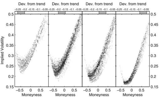
Other characteristic features make de nitely different the implied volatility

surface of the market from the constant Black&Scholes volatility: for example, in

Figure 1.1 we show the dependence of the implied volatility of options on the

S&P500 index, with respect to the so-called “deviation from trend” of the

underly-ing asset, de ned as the difference between the current price and a weighted mean

of historical prices. Intuitively this parameter indicates if there have been sudden

large movements of the quotation of the underlying asset.

Finally we note that the implied volatility depends also on time in absolute

terms: indeed, it is well known that the shape of the implied volatility surface on

the S&P500 index has signi cantly changed from the beginning of the eighties

until today. The market crash of 19 October 1987 may be taken as the date

mark-ing the end of at volatility surfaces. This also re ects the fact that, though based

on the same mathematical and probabilistic tools, the modeling of nancial and,

for instance, physical phenomena are essentially different: indeed, the nancial

dynamics strictly depends on the behaviour and beliefs of investors and therefore,

differently from the general laws in physics, may vary drastically over time.

(22)

Fig. 1.1. Effect of the deviation from trend on the implied volatility. The

volatility smiles for options on the S&P500 index are grouped for

differ-ent values of the deviation, as indicated on top of each box

The Black&Scholes model and its pricing formula are wrong: the analysis of the

implied volatility surface makes it evident that the Black&Scholes model is not

realistic. As often quoted, the implied volatility is the wrong number to put in the

wrong formula to obtain the right price: more precisely, we could say that

nowa-days Black&Scholes is the language of the market (since prices are quoted in

terms of implied volatility), but usually it is not the model really used by investors

to price and hedge derivatives. It comes at rst as a surprise to see this apparently

irrelevant number being constantly used by traders. Why should it deserve so

much attention?

A rst answer is pointed out in [Lee05]. "[...] it is helpful to regard the

Black-&Scholes implied volatility as a language in which to express an option price.

Use of this language does not entail any belief that volatility is actually constant.

A relevant analogy is the quotation of a discount bond price by giving its yield to

maturity, which is the interest rate such that the observed bond price is recovered

by the usual constant interest rate bond pricing formula. In no way does the use

or study of bond yields entail a belief that interest rates are actually constant. As

yield to maturity is just an alternative way of expressing a bond price, so is

implied volatility just an alternative way of expressing an option price.

The language of implied volatility is, moreover, a useful alternative to raw

prices. It gives a metric by which option prices can be compared across different

strikes, maturities, underlyings, and observation times; and by which market

prices can be compared to assessments of fair value. It is a standard in industry,

to the extent that traders quote option prices in "vol" points, and exchanges

update implied volatility indices in real time."

Indeed the use of the Black&Scholes model poses some not merely theoretical

problem: for instance, let us suppose that, despite all the evidence against the

Black-Scholes model, we wish to use it anyway. Then we have seen that we have

to face the problem of the choice of the volatility parameter for the model. If we

use the historical volatility, we might get quotations that are “out of the market”,

especially when compared with those obtained from the market-volatility surface

in the extreme “in” and “out of money” regions. On the other hand, if we want to

use the implied volatility, we have to face the problem of choosing one value

among all the values given by the market, since the volatility surface is not “ at”.

Evidently, if our goal is to price and hedge a plain vanilla option, with strike,

say, K and maturity, say, T , the most natural idea is to use the implied volatility

corresponding to

HK, TL. But the problem does not seem to be easily solvable if

we are interested in the pricing and hedging of an exotic derivative: for example,

(23)

Indeed the use of the Black&Scholes model poses some not merely theoretical

problem: for instance, let us suppose that, despite all the evidence against the

Black-Scholes model, we wish to use it anyway. Then we have seen that we have

to face the problem of the choice of the volatility parameter for the model. If we

use the historical volatility, we might get quotations that are “out of the market”,

especially when compared with those obtained from the market-volatility surface

in the extreme “in” and “out of money” regions. On the other hand, if we want to

use the implied volatility, we have to face the problem of choosing one value

among all the values given by the market, since the volatility surface is not “ at”.

Evidently, if our goal is to price and hedge a plain vanilla option, with strike,

say, K and maturity, say, T , the most natural idea is to use the implied volatility

corresponding to

HK, TL. But the problem does not seem to be easily solvable if

we are interested in the pricing and hedging of an exotic derivative: for example,

if the derivative does not have a unique maturity (e.g. a Bermudan option) or if a

xed strike does not appear in the payoff (e.g., an Asian option with oating

strike).

These problems make it necessary to introduce more sophisticated models than

the Black&Scholes one, that can be calibrated in such a way that it is possible to

price plain vanilla options in accordance with the implied volatility surface of the

market. In this way such models can give prices to exotic derivatives that are

consistent with the market Call and Put prices. This result is not particularly

difficult and can be obtained by various models with non-constant volatility. A

second goal that poses many more delicate questions and is still a research topic

consists in nding a model that gives the “best” solution to the hedging problem

and that is stable with respect to perturbations of the value of the parameters

involved ([SST04] and [Con06]).

Instead of a constant volatility, one can posit a volatility that is a function of the

spot process itself. This way, the spot process is a Markov process solution of a

stochastic differential equation, and we obtain the so-called local volatility (LV)

models ([Bre06], [Cre03], [DK94], [DKC96], [DKK96], [Dup93], [Dup94],

[Eng06], [Gat06], [Reb04], [Wil06]). A more general approach consists in a

volatility being a stochastic process on its own. In such a case the spot process

alone is no longer Markov and such models are often called stochastic volatility

(SV) models ([DK98], [HKLW02], [Hes93], [HW87]). Finally, people have

further proposed to introduce jumps in the spot process (Lévy models: [AA00],

[Mer76]). These idea can of course be combined with any of the other ones.

Stochastic volatility processes were introduced by Hull and White [HW87]. In it

the volatility itself is a process that satis es a stochastic differential equation. The

most famous stochastic volatility models are the Heston model [Hes93] and the

SABR model [HKLW02]. How these models cause the volatility skew in the

market is discussed in ([DK98], [HKLW02]).

Jump-diffusion models were rst introduced by Merton [Mer76]. These models

incorporate discontinuous jumps in the underlying asset price. This resembles

reality were events can have sudden impacts on asset prices. How this explains the

volatility skew is described in [AA00].

The local volatility model assumes the volatility is a deterministic function of

the asset price and time. It came into existence when Dupire ([Dup93], [Dup94])

showed that, in the presence of volatility skews, consistent models can be built if

(24)

The local volatility model assumes the volatility is a deterministic function of

the asset price and time. It came into existence when Dupire ([Dup93], [Dup94])

showed that, in the presence of volatility skews, consistent models can be built if

the asset price process is assumed to have the following dynamics under the risk

neutral probability measure Q

â S

_t

S

t

=

Hr

_t

- q

_t

L ât + sHt, S

_t

L âW

_t

where the volatility is now a deterministic function of time and the asset price and

r

t

and q

t

denote the continuously compounded short rate and dividend

respec-tively. In this case the diffusion process is usually referred to as local volatility.

These models attempt to explain the various empirical deviations from the

Black&Scholes model by introducing additional degrees of freedom in the model

such as a local volatility function, a stochastic diffusion coef cient, jump

intensi-ties, jump amplitudes etc. However, these additional parameters describe the

in nitesimal stochastic evolution of the underlying asset while the market usually

quotes options directly in terms of their market-implied volatilities which are

global quantities.

In order to see whether the model reproduces empirical observations, one has to

relate these two representations: the in nitesimal description via a stochastic

differential equation on one hand, and the market description via implied

volatili-ties on the other hand.

However, in the majority of these models it is impossible to compute directly

the shape of the implied volatility surface in terms of the model parameters.

Although it is possible to compute the implied volatility surface numerically,

these numerical studies show that simple jump processes and one factor stochastic

volatility models do not reproduce correctly the pro les of empirically observed

implied volatility surfaces and smiles ([BCC97], [DS99], [Tom01]).

This problem is also re ected in the dif culty in 'calibrating' model parameters

simultaneously to a set of liquid option prices on a given date: if the number of

input option prices exceeds the number of parameters (which should be the case

for a parsimonious model) a con ict arises between different calibration

con-straints since the implied volatility pattern predicted by the model does not

corre-spond to the empirically observed one. This problem, already present at the static

level, becomes more acute if one examines the consistency of model dynamics

with those observed in the options market. While a model with a large number of

parameters, such as a non-parametric local volatility function, may calibrate well

the strike pro le and term structure of options on a given day, the same model

parameters might give a poor t at the next date, creating the need for constant

re-calibration of the model. Examples of such inconsistencies over time have been

documented for the implied-tree approach by Dumas et al ([DFW98]). This time

instability of model parameters leads to large variations in sensitivities and hedge

parameters, which is problematic for risk management applications.

The inability of models based on the underlying asset to describe dynamic

behaviour of option prices or their implied volatilities is not, however, simply due

to the mis-speci cation of the underlying stochastic process. There is a deeper

reason: since the creation of organized option markets in 1973, these markets have

(25)

The inability of models based on the underlying asset to describe dynamic

behaviour of option prices or their implied volatilities is not, however, simply due

to the mis-speci cation of the underlying stochastic process. There is a deeper

reason: since the creation of organized option markets in 1973, these markets have

become increasingly autonomous and option prices are driven, in addition to

movements in the underlying asset, also by internal supply and demand in the

options market.

This fact is also supported by recent empirical evidence of violations of

qualita-tive dynamical relations between options and their underlying ([BCC00]). This

observation can be accounted for by introducing sources of randomness which are

speci c to the options market and which are not present in the underlying asset

dynamics.

(26)

(27)

C H A P T E R

2

s s s 2

Lorig, Pagliarani and

Pascucci’s Work

When it comes to the options market, particularly the Foreign Exchange (FX)

options market, the valuation of barrier options and other exotic options is

differ-ent from that of vanilla options as prices of these exotic options are not only

dependent on the dynamics of the vanilla market quotes.

Neither local volatility (LV) nor stochastic volatility (SV) models are able to t

empirically observed implied volatility levels over the full range of strikes an

maturities. This has led to the development of local- stochastic volatility (LSV)

models, which combine the features of LV and SV models by describing the

instantaneous volatility of an underlying S by a function f

HS

t

, Z

t

L where Z is some

auxiliary, possibly multidimensional, stochastic process (see, for instance,

[Lip02], [AN04], [Ewa05], [HeLa09] and [Cla10]).

Local volatility and stochastic volatility models are actually calibrated to only

market vanilla options, and hence do not have the exibility to capture the

dynam-ics of exotic options. Therefore, hybrid use of both models was proposed. For

example, a linear average of prices from both local volatility and stochastic

volatil-ity models was employed by practitioners as to price exotic options (see [TF10]),

whereas there is no theocratical point of this approach.

The general dynamics of the hybrid stochastic-local volatility model are

(2.1)

â S

t

= m

1 HS

t

, t

L ât + LHS

t

, t

L s

1 HS

t

, Z

t

, t

L âW

t

1 ,

â Z

t

= m

2 HZ

t

, t

L ât + s

2 HZ

t

, t

L âW

t

2 ,

â W

t

1 × â W

t

2 = r â t

with the correlation - 1 < r < 1. L

HS

t

, t

L is called leverage function, which is to be

determined by market information in order to control the weights of local

volatil-ity and stochastic volatilvolatil-ity. If the price process of the new LSV model could

mimic that of the local volatility model, then the two models should generate the

same pricing results for European options. In order to achieve this goal, we need

to match the diffusion terms of the two models. We refer to [Gyo86], [Kle02],

[Dup04] and [Tac11] for more theoretical backgrounds.

Compared to their LV and SV counterparts, LSV models produce implied

volatility surfaces that more closely match those observed in the market.

How-ever, LSV models rarely allow for exact formulas for option prices. Thus, LSV

models present two challenges. First, given an LSV model, can one nd accurate

(28)

volatility surfaces that more closely match those observed in the market.

How-ever, LSV models rarely allow for exact formulas for option prices. Thus, LSV

models present two challenges. First, given an LSV model, can one nd accurate

closed-form approximations for option prices? Second, given approximate option

prices, can one nd accurate closed-form approximations for implied volatilities?

In the class of the stochastic-local volatility model, there are different

view-points of modeling and calibration approaches. Jex, Henderson and Wang

([JHW99]) used a trinomial tree method. Lipton ([Lip02]) proposed a so-called

universal volatility model, which combines local volatility and stochastic

volatil-ity. Ren, Madan and Qian ([RMQ07]) used a log-normal model for spot process

and volatility process with zero correlation. Tataru & Fisher ([TF10]) also

sug-gested a term-structure model with log-normal process for volatility, which they

believe describes the realistic market dynamics. Moreover, both Ren et al.

([RMQ07]) and Tataru and Fisher ([TF10]) constructed the volatility process as a

stochastic multiplier (around 1) imposed on local volatility. Henry-Labordère

([HeLa09]) and van der Stoep, Grzelak and Oosterlee ([vdSGO13]) proposed

Monte Carlo based approaches for calibration. Choi, Fouque and Kim ([CFK12])

used a stochastic volatility following a mean-reverting Ornstein-Uhlenbeck

pro-cess. Deelstra & Rayée ([DR12]) suggested a LSV model with stochastic interest

rate to price long-dated FX options.

In the area of pricing, there have been a number or recent developments. An

exhaustive review of LSV pricing approximations would be prohibitive. However,

we also mention the following: Pagliarani and Pascucci ([PP13]) added jumps to a

LSV model, but also a general local volatility to the Heston model obtaining a

Fourier-like representation for approximate option prices. Rather than

non-paramet-ric construction of the leverage function, Murex ([Mur11]) and Wystup ([Wys11])

constructed a parametric approach with a forward process. Lorig ([Lor12]) added

multi scale stochastic volatility to general scalar diffusions, and thus obtains

analytically tractable eigenfunction approximations for options prices. Finally,

Lorig, Pagliarani and Pascucci ([LPP13]) proposed an asymptotic expansion for

the transition probability of general parametric hybrid volatility models.

Typically, unobservable LSV (or SV or LV) model parameters are obtained by

calibrating these models to implied volatilities that are observed on the market. To

do this, one must nd model-induced implied volatilities over a range of strikes

and maturities. Computing model-induced implied volatilities from option prices

by inverting the Black Scholes formula numerically is a computationally intensive

task, and therefore, not suitable for the purposes of calibration. For this reason

closed-form approximations for model-induced implied volatilities are needed. A

number of different approach have been taken for computing approximate implied

volatilities in LV, SV and LSV models.

Concerning LV models, perhaps the earliest and most well-known implied

volatility result is due to Hagan and Woodward ([HW99]), who used singular

perturbation methods to obtain an implied volatility expansion for general LV

models. For certain models (e.g., CEV) they obtained closed-form

approxima-tions. More recently, Lorig ([Lor13]) used regular perturbation methods to obtain

an implied volatility expansion when a LV model can be written as a regular

perturbation around Black-Scholes. Jacquier and Lorig ([JL13]) extended and

re ned the results of Lorig ([Lor13]) to nd closed-form approximations of

(29)

models. For certain models (e.g., CEV) they obtained closed-form

approxima-tions. More recently, Lorig ([Lor13]) used regular perturbation methods to obtain

an implied volatility expansion when a LV model can be written as a regular

perturbation around Black-Scholes. Jacquier and Lorig ([JL13]) extended and

re ned the results of Lorig ([Lor13]) to nd closed-form approximations of

implied volatility for local Lévy-type models with jumps. Gatheral, Hsu,

Lau-rence, Ouyang, and Wang ([GHLO12]) examined the small-time asymptotics of

implied volatility for LV models using heat kernel methods.

There is no shortage of implied volatility results for SV models either. Fouque,

Lorig, and Sircar ([FLS12]) (see also [FPSS11]) derived an asymptotic expansion

for general multiscale stochastic volatility models using combined singular and

regular perturbation theory. Forde and Jacquier ([FJ11]) used the

Freidlin-Wentzell theory of large deviations for SDEs to obtain the small-time behavior of

implied volatility for general stochastic volatility models with zero correlation.

Their work added mathematical rigor to previous work by Lewis ([Lew07]). Forde

and Jacquier ([FJ09]) used large deviation techniques to obtain the small-time

behavior of implied volatility in the Heston model (with correlation). They further

re ned these results in [FJL12].

Concerning LSV models, perhaps the most well-known implied volatility result

is due to Hagan, et al. ([HKLW02]), who used WKB approximation methods to

obtain implied volatility asymptotics in a LSV model with a CEV-like factor of

local volatility and a GBM-like factor of non-local volatility (i.e., the SABR

model). More recently, Henry-Labordère ([HeLa05]) used a heat kernel expansion

on a Riemann manifold to derive rst order asymptotics for implied volatility for

any LSV model. As an example, he introduced the l-SABR model, which is a

LSV model with a mean reverting non-local factor of volatility, and obtained

closed form asymptotic formulas for implied volatility in this setting. See also

[HeLa09a]. There are also some model-free results concerning the extreme-strike

behavior of implied volatility. Most notably, we mention the work of Lee

([Lee04]) and Gao and Lee ([GL11]).

In this chapter we talk about local stochastic volatility (LSV) models, and in

particular, we’re going to obtain a price and an implied volatility expansion for

these models; in doing so, we define the problem and the method of resolution as

presented in the works of Lorig, Pagliarani and Pascucci ([LPP13] and [LPP13a]),

following also other works of the same authors ([LPP13b] and [PP12]) and

propos-ing some method’s improvements.

In order to guarantee consistence in our work, we use from the beginning the

notation presented in [LPP13b] which is more general and flexible, but whereas in

all of these papers the risk-free interest rate is set to zero, here we consider a

deterministic interest rates.

In the next chapter we consider the particular case covered in [LPP13a] and we

implement the obtained implied volatility expansion in some numerical tests,

optimizing the code and going further in the computation than in ([LPP13]) in

order to prove whether the approximation converges and at which order we could

and should stop.

(30)

3 Local Stochastic Volatility (LSV) models

As in [LPP13], we consider general LSV models. For these models, they derive

a family of closed-form asymptotic expansions for transition densities, option

prices and implied volatilities. The presented method most closely follows that of

Forward implied volatility expansions in LSV models

facoltà di scienze matematiche, fisiche e naturali

Corso di Laurea Magistrale in Matematica

Forward Implied Volatility Expansions

in LSV models

Tesi di Laurea in Matematica Finanziaria

Relatore

Presentato da:

Chiar.mo Prof.

Paolo Martini

Andrea Pascucci

II Sessione

Forward Implied Volatility

Expansions in LSV models

Ai miei genitori

Alla mia pulce Fabiana

Table of Contents

x

Introduction

Chapter 1

1

B & S Model and IV problem

1

1 The Black & Scholes Model

1

1.1 Lognormal Property of Stock Prices

2

1.2 Black - Scholes - Merton differential equations

4

1.3 Risk - Neutral Valuation

5

1.4 Black & Scholes Pricing Formulas

6

1.5 Consistence of Black & Scholes Formulas

7

2 Implied Volatility

8

2.1 The Implied Volatility Problem

Chapter 2

15

Lorig, Pagliarani and Pascucci

÷s Work

18

3 Local Stochastic Volatility

HLSVL models

19

3.1 General local - stochastic volatility models

19

4 Transition density and option pricing PDE

22

5 Expansion basis

23

5.1 Taylor Expansion

23

5.2 Enhanced Taylor Expansion

24

5.3 Hermite Expansion

24

6 Density and option price expansions

26

7 Implied volatility expansions

27

7.1 Implied volatility expansions from price expansions

30

7.2 Implied volatility when

option prices are given by Theorem

H6L

Chapter 3

33

Numerical Tests on Implied Volatility

33

8 A Taylor series approach

34

8.1 CEV local volatility model

36

8.1.1 First Set : d = 0.25, b = 0.8

50

8.1.2 Second Set : d = 0.25, b = 0.2

56

8.1.3 Third Set : d = 0.4, b = 0.5