Laser Beam Characterization by Imaging for Product Inspection

UNIVERSITÀ DI PISA

Facoltà di Ingegneria

Laurea Specialistica in Ingegneria dell’Automazione

Tesi di laurea

Candidato:

Filippo Bisti

_____Firma__________

Relatori:

Prof. Michele Lanzetta _____Firma__________

Ing. Lorenzo Pollini

_____Firma__________

Prof. Michael Schmidt _____Firma__________

Prof. Giovanni Tantussi _____Firma__________

LASER BEAM CHARACTERIZATION BY

IMAGING FOR PRODUCT INSPECTION

Sessione di Laurea del 02/03/2012 Anno accademico 2010/2011

ABSTRACT

This thesis discusses the design and the realization of a Beam Propagation Analyzer apparatus and the application of laser beams in surface characterization. Most of this work has been performed at the University of Erlangen-Nürnberg, Chair of Photonics Technologies (Germany).

Today laser beams are widely used in a large number of industrial applications. Mechanical Machining, Electronics Industries, Communication Engineering and Medical Application are some areas in which the laser technologies play a key role. The design of optical system is treated with powerful simulation software but it requires at the same time a good knowledge of basic rules of Optics. These beam propagation and transformation can be defined by two critical parameters: the beam waist (the smallest beam radius achieved in the beam trajectory) and the divergence angle (the ratio at which the beam enlarges far away from the waist). These parameters are strongly related and they are important indicators of the beam quality. The beam quality can be measured with an apparatus composed by a beam profiler (instrument able to measure the intensity profile of the beam) and a translation stage that permits the measurement of the beam intensity at different positions. Such a type of apparatus has been realized.

The apparatus has been designed and realized with commercial elements, the hardware interacts with the laser beam and PC software controls the image acquisitions and analyzes the data. The developed apparatus characterizes the quality of low power laser beams in the range ! = 500 ÷ 1000  !" and !_! = 0.8 ÷ 2.5  !! collecting images of the beam sections along the propagation axis. The image analysis returns the beam parameters !_!!, !_!!, !_!", !_!", !_!! _{and !}

!!.

Laser beams are also widely used in surface characterization. A novel method, based on the speckle effect and normally applied in roughness characterization of metallic surfaces, is tested on Carrara marble stones to investigate a possible new field of applications.

ACKNOWLEDGEMENTS

I wish to thank Prof. Michele Lanzetta for the opportunity to realize this work in a foreign institute. I want also thank Ph.D Ilya Alexeev for the support and the suggestions received during the period spent in Erlangen.

I would like to give special thanks to Prof. Giovanni Tantussi, for his help in the preparation and characterization of the specimens.

1.

LASER AND BEAM QUALITY

High power lasers in manufacturing are used for cutting, welding, marking, drilling, surface treatments and powder processing on a variety of materials ranging from metal, to polymers and natural materials like leather or stone. Low power lasers are increasingly applied for optical inspection, by measuring position, distance, speed and surface properties like roughness and gloss. An apparatus has been developed that controls the beam path and measures these properties with an image analysis.

1.1 Laser Parameters

1.1.1 Beam Quality

The most common parameter used to quantify the beam quality is the !! _{parameter. As}

described in (Siegman & Ginzton, 1997), in a resumption of the previous work (Siegman, 1993), every laser beam can be characterized by the factor called !!_{, which is related to the capability to}

focalize the laser in a narrow spot with a predetermined divergence angle. The best possible beam quality is achieved for a diffraction-limited Gaussian beam (particular solution of the of equation wave), having !! _{= 1. Many lasers approach this}

value, especially the low power single mode like some diode lasers. On the other hand, high power lasers can have a very large !! _{of more than 100}

or even well above 1000.

Figure 1.1 shows a scheme of welding process. A better beam quality permits to locate the welding head farther from the working surface, avoiding possible damages. In laser delivery systems the beams with high quality propagate with a narrower beam size, so smaller and cheaper optics can be used. These beams remain collimated for a longer distance, increasing the tolerance for longitudinal alignment. (Paschotta, 2011).

A laser beam is normally described referring to an ideal Gaussian beam.

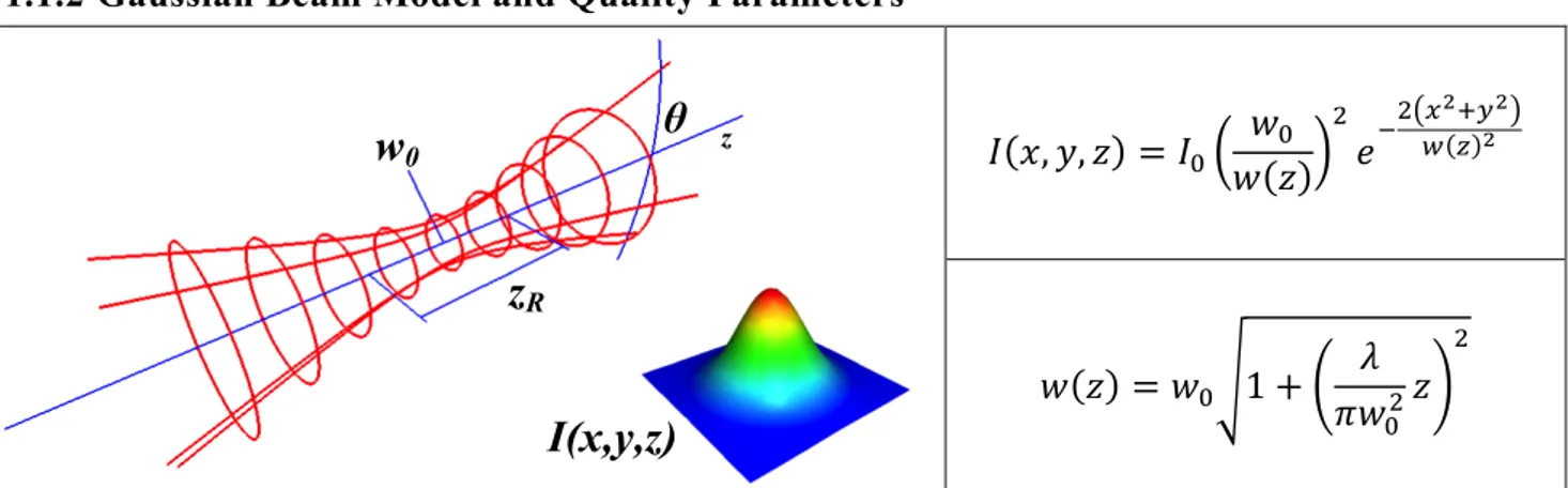
1.1.2 Gaussian Beam Model and Quality Parameters

! !, !, ! = !_! !! ! ! ! !! ! !!!!! ! !! ! ! = !_! 1 + ! !!_!!! !

Figure 1.2 Gaussian Beam Propagation Functions.

A laser beam is characterized by its transversal intensity distribution in the planes perpendicular to the beam axis. The fundamental model for a laser beam is the Gaussian beam. In Figure 1.2 are provided the fundamental equations characterizing the shape of a Gaussian beam. The intensity function !(!, !, !) is the time-averaged power density. The beam radius ! ! is the width of the

Figure 1.1 Beam Quality Effect in Welding !"#$%&'()%*+(,"-.% /0_12% 345%&'()%*+(,"-.%_/0_662% !"# !$# %"&%$# !% !"'!$# %"# %$# ()*+,#-./,0+# 1,,)23)4+2#-/,!)0+# 5+ )6# 7 3,+ 08 .9 # (+9*# (+9*#

w

z

θ

I(x,y,z)

beam in the propagation axis transversal plane. Three parameters define a Gaussian Beam:

Beam Waist !! The parameter !_{reached by the beam along its path.} ! is the beam waist, the smallest radius

Divergence Angle ! ≅ !"# ! = ! !!_!  

The region in which !"#!→∞! ! = !" is called far field. A small beam waist implies a large divergence

angle, and vice versa. Rayleigh Range !_! = !

!!!!  

At a distance equal to !_! from the beam waist, the beam radius is ! !! = 2!!. The interval centered in !! and

with semi-aperture of !_!,  is called near field.

1.1.3 Real Beams Characterization and !! _Parameter

The beam quality !! _{parameter adapts the Gaussian model to a real beam. It quantifies the}

quality in relation to the similarities between a real beam and a Gaussian beam. It is defined as: !! ₌ !"!!"#$ !"!_!"#$$%"&= !_!!_! !_!! = !"_!! !

The !! _{is larger than one for any real beam and represents the ratio between the beam waist}

radius of the real beam and the beam waist radius of a Gaussian beam with the same divergence angle. The !! _{defines the shape of the real beam along the z-axis.}

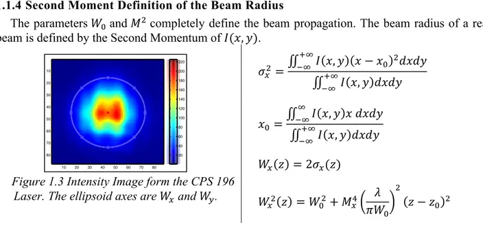
1.1.4 Second Moment Definition of the Beam Radius

The parameters !_! and !! _{completely define the beam propagation. The beam radius of a real}

beam is defined by the Second Momentum of !(!, !).

Figure 1.3 Intensity Image form the CPS 196

Laser. The ellipsoid axes are !_! and !_!.

!!! = ! !, ! ! − !_! !_!"!# !! !! ! !, ! !"!# !! !!   !_! = ! !, ! !  !"!# ! !! ! !, ! !"!# !! !!   !_! ! = 2!_!(!) !!! ! = !!! + !!! ! !!_! ! ! − !! !

The characterization of these parameters is the task of the developed apparatus.

2.

DESIGN OF THE OPTICAL SYSTEM

The design of the apparatus consists in the project of the hardware layout based on the laser source specifications and on the camera limitations defined with computer simulations.

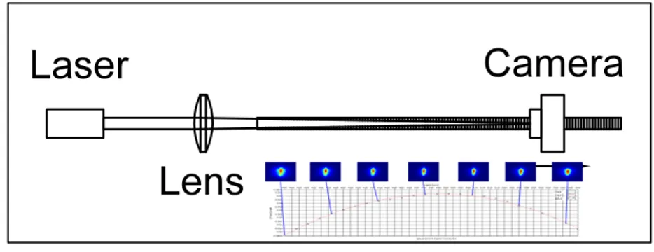
2.1 Characterization Strategy

The characterization of a real laser beam requires a several beam scans along the beam path. A possible layout is presented in Figure 2.1. The laser beam is focalized by a lens and a camera records images the path. The collected scans are then analyzed to extract the beam parameters.

10 20 30 40 50 60 70 80 10 20 30 40 50 60 70 80 20 40 60 80 100 120 140 160 180 200 220

Figure 2.1 Schematic Beam Characterization Hardware

There are two applicable algorithms for the parameter characterization. The beam waist and the divergence angle can be estimated separately or the estimated beam radii can be fitted with a parabolic function and the parameters are then calculated from the parabola coefficient.

2.2 Beam Profiling with CMOS Camera

Some works describe methods for the analysis of the beam profile with camera sensors (Schweinsberg & Van Woerkom, 1999), (Alsultanny, 2006), (Andrews, Gupta, Bose, & Kumar, 2007) and a general review of the commercial instruments is available in (Roundy, 2005).

The CMOS camera DCC1545 is selected for the apparatus. The resolution of the CMOS camera is critical for the beam radius measurement. Simulations were performed to investigate the effect on the estimation of the beam radius caused by the spatial discretization and the intensity level quantization. Complex camera models are discussed in (Micron, 2010).

2.2.1 Image Generation and Analysis

The most important property to be defined is the smaller beam radius that the apparatus can measure. Each pixel is treated like an integrator of the light intensity to simulate the image acquisition. The output signal !_!"!"" _{is proportional to the energy !}

!"  collected during the exposure

time. The energy !_!" is then scaled to set the output range between 0 and 255, simulating the compensation in the exposure time to avoid image saturation. Finally, these values are quantized and a random noise !_!!"" _{between 0 and 5 levels is added to generate pseudo-images.}

!!" = ! ! !, ! !"   !!" ! !  !" !_!"!"" _{= !"#$8} 255 !"# ! !!" + !!!""

The random noise in the zones far from the beam center generates deviations in the radius estimation. The estimation algorithm implements the second moment definition for the radius as:

Divergence Procedure (ISO 11146):

1. Set the measuring instrument to estimate the radius with the second moment method

2. Measure the beam radius at 5 axial positions in the near field

3. Measure the beam radius at 5 axial positions in the far field

4. Fit the data couples !, ! ! in the near field with

a parabolic function to estimate !₀

5. Fit the data couples in the far field with a linear function to estimate !

6. !2= !"!0

! , !! = !!₀!

!!2

Second Moment Procedure (Siegman & Ginzton, 1997): 1. Set the measuring instrument to estimate the radius

with the second moment method

2. Measure the beam radius at several positions along the propagation axes

3. Fit the data with a parabolic function:

! ! !_{= !!}!_{+ !" + !}

4. Calculate the beam waist with the formula:

!₀= −! 4! ;  ! 2 _{= (}!!0 ! ) !;  !!  = !2_!!!" !!!

!_!! _{= !} !"!"" ! − !! !!!"# ! !!! ! !!! , !!"# = 0, !_!" < !"# 1, !_!" ≥ !"#  

The Figure 2.2 shows that the best cutoff value must be near to the peak value of the noise.

Figure 2.2 Cutoff Effect with Random Noise.

A too large value would decrease too much the estimated beam radius. The enlargement of the beam radius also improves the estimation because the sensor has a finite area so the spatial SNR increases. Figure 2.2 shows that a suitable choice for the cutoff level is a value near to the peak of the supposed random noise.

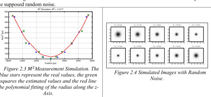
Figure 2.3 !!_{Measurement Simulation. The}

blue stars represent the real values, the green squares the estimated values and the red line the polynomial fitting of the radius along the

z-Axis.

Figure 2.4 Simulated Images with Random Noise.

Finally, general simulations of the entire process of estimation have been performed. Errors in the positions of the images are introduced and the radii are estimated with the previous algorithm. Figure 2.3 shows the results for a simulated beam with !! _{= 1. As it can be seen from this and}

other simulations, in spite of the noises in both position and radius values, the estimated value of the !! _{is close to the real value. The simulated images are displayed in Figure 2.4.}

2.2.2 Simulation results

From these simulations a cutoff value of 5 levels is selected. The minimum beam radius is set to 10 pixels, which is equal to 52  !" for the employed camera.

1 2 3 4 5 6 7 8 9 10 10ï1 100 101 102 103 104

Cutoff Level Effect

Real Radius [px] Relative Error ¡ % Cutoff Level = 0 Cutoff Level = 2 Cutoff Level = 4 Cutoff Level = 6 Cutoff Level = 8 ï6000 ï4000 ï2000 0 2000 4000 6000 100 150 200 250 300 350 400 450 500 550 M2 _{Simulation: M}2 _{= 1.0177} Position [px] W(z) 2 [px] Wx = 22.6 [px] 20406080 100 20 40 60 80 100 Wx = 19.1 [px] 20406080 100 20 40 60 80 100 Wx = 15.8 [px] 20406080 100 20 40 60 80 100 Wx = 12.9 [px] 20406080 100 20 40 60 80 100 Wx = 10.9 [px] 20406080 100 20 40 60 80 100 Wx = 10.1 [px] 20406080 100 20 40 60 80 100 Wx = 10.9 [px] 20406080 100 20 40 60 80 100 Wx = 12.9 [px] 20406080 100 20 40 60 80 100 Wx = 15.8 [px] 20406080 100 20 40 60 80 100 Wx = 19.0 [px] 20406080 100 20 40 60 80 100

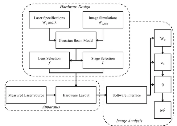
The simulation results and the laser specifications allow the hardware design as depicted in Figure 2.5.

Figure 2.5 General Scheme of the Apparatus and its Design.

2.3 Hardware Design

The hardware layout in Figure 2.1 causes waist of space and problem with the camera movements. These issues are solved with the designed layout. The movable part is a prism on a rail guide, allowing save of space and no camera motion.

Figure 2.6 Scheme of the Hardware Layout. The camera records the beam intensity. The movement of the prism permits the collection of images along the beam path.

The simulations on the camera and the properties of the low power lasers define the specifications to be fulfilled by the apparatus: ! = 500 ÷ 1000  !" , FWHM: 0.8 ÷ 2  !! , 2!_! = 52  !". From these specifications a focalizing lens and the translation stage length are selected. Figure 2.6 shows a conceptual scheme of the apparatus parts.

Image Simulations W0,min

Laser Specifications

W0 and !

Gaussian Beam Model

Stage Selection

L

Lens Selection

f

Hardware Layout

Measured Laser Source Software Interface

W0 " z_R M2 Hardware Design Apparatus Image Analysis

Aligning Optics Focusing Lens

Camera I(x,y)

Prism on Rail Guide

Position: z Laser Source Hardware Layout Acquisition Software Analysis Software PC Apparatus

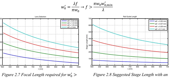
2.4 Lens and Stage Length Selection

The beam has to be focused to characterize the !!_{. The camera resolution imposes the minimum}

measurable beam waist. The beam waist is related to the Rayleigh range that should be not too large to save space on the platform. For a Gaussian beam, under certain conditions (Self, 1983), it holds:

!_!! ₌ !"

!!_! → ! >

!!_!!_!,!"#!

!  

Figure 2.7 Focal Length required for !_!! _>

52  !".

Figure 2.8 Suggested Stage Length with an Optimal Lens.

The lens is selected analyzing the behavior of the beam waist and the Rayleigh range against the variation of the wavelength and the beam initial radius. The results are plotted in the graph in Figure 2.7. An analogue consideration can be done for the minimal stage length required. Considering the selection of an optimal lens accomplished with the graph in Figure 2.7, the minimal beam waist will be larger than 52  !". The rail length must be 5 times the Rayleigh range to perform an accurate measure. Figure 2.8 reports the suggested translation stage lengths.

2.5 Hardware Layout

Figure 2.9 CAD Model of the Beam Propagation Analyzer Apparatus.

In a real application it is very difficult, even impossible, to move the laser source to adjust the

500 550 600 650 700 750 800 850 900 950 1000 0 100 200 300 400 500 600 700

Rail Guide Length

h [nm] Stage Length [mm] w0, _{= 0.05 mm} w0, _{= 0.07 mm} w0, _{= 0.09 mm} w0, _{= 0.1 mm} 500 550 600 650 700 750 800 850 900 950 1000 100 200 300 400 500 600 700 Lens Selection h [nm] f [mm] w0 = 0.8 mm w0 = 1.2 mm w0 = 1.6 mm w0 = 2 mm

beam path to match a determinate trajectory. The best way to redirect the beam along a predetermined trajectory consists in building an optical track with a series of optics elements. The CAD model of the apparatus, realized with SolidWorks, is visualized in Figure 2.9. The request of a long rail guide length is managed introducing a right angle prism used as retro-reflector to modify the length of the beam path.

The beam travels through the air from the laser source (1) to the camera (10), following an optical track formed by a periscope (2), a mirror (3) and a prism (7). The prism is supported by the translation stage (8) on the rail guide (9), allowing the movement of the prism along the propagation axis. Before the beam strikes the prism it is focalized by a convex lens. The prism position can be read on a ruler fixed along the rail guide (9s) or on the micrometer of the translation stage (8s). The prism is used like a retro-reflector; it sends the beam back in the same direction of the incident beam. In this way, the movement of the prism results doubled in the length of the beam path, permitting to save space in the hardware. In this apparatus, the measures are performed on a diode laser source.

3.

BEAM CHARACTERIZATION SOFTWARE

The tasks of the software are depicted in Figure 3.1. The software is divided in two subprograms.

Figure 3.1 Scheme of the Software. The images are stored with the positions and then analyzed.

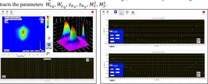
The first collects the images and controls the camera settings; the second analyzes the images and extracts the parameters  !_!!, !_!!, !_!!, !_!!, !_!!_{, !}

!!.

Figure 3.2 Acquisition Software. Figure 3.3 Analysis Software.

Apparatus

Camera Controls

Saturation Test Project

Take Images

Insert Positions

Beam Widths Extraction Data Fitting and

Parameter Calculation W0, zR, !, M2

Analysis Software Acquisition Software

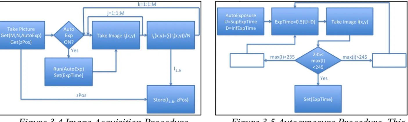
3.1 Image Acquisition

Figure 3.4 and Figure 3.5 describe the procedures for the image acquisition performed with the Acquisition software (Figure 3.2).

Figure 3.4 Image Acquisition Procedure. Several images are stored at each position.

Figure 3.5 Autoexposure Procedure. This procedure automatically set the exposure time

to avoid image saturation.

For each position several pictures are taken, which are the average of some camera images as shown in Figure 3.4. The exposure time is modified to prevent image saturation. The program returns a project which is a collection of images related with the positions.

3.2 Image Analysis

The Analysis software (Figure 3.3) elaborates the images extracting the beam radii and reconstructing the propagation functions. Two methods are available to estimate the beam parameters and to calculate the !! _{which implement the table in 2.1.}

The report file produced by the Analysis software is provided below.

• Project Name: 500mm_n2_m1 • Pixel Dimension: 5.2 µm • Laser Wavelength: 635 nm • Method: S^2 W0 [mm] RL [mm] M2 WL [nm] X 0.160 70.837 3.594 635.000 Y 0.249 148.682 4.113 635.000 d [mm] x0 [px] y0 [px] Sx [px] Sy [px] 445.000 609.870 443.075 27.278 29.262 449.000 613.031 449.323 25.935 28.660 … … … … …

Figure 3.6 Graphs of the Radius Propagation

4.

TEST OF THE APPARATUS

The device and the software were tested on a !"#" red laser and on the diode laser CPS196, acquired from Thorlabs. Tests on real images evidence a small relative standard deviation in the radius estimation if an adequate cutoff level is selected (Figure 4.1 and Figure 4.2).

Image Acquisition !"#$%&'()*+$% ,$)-./0/1*)23456% ,$)-7&286% 1*)2 345% 90:% !"#$%;<"=$%;>-4/?6% ;#-4/?6@A-;>-4/?66B0% C*D-1*)23456% E$)-345!'<$6% E)2+$-;FGG0/%7&286% >@FHFH.% #@FHFH.% I$8% 7&28% ;FGG0%

Laser Beam Propagation Analysis

The procedure executed to acquire an image:

AutoExposure !"#$%&'$(")*+ ,-."'%&'/01*+ 2-345%&'/01*+ 6789+ 1:&;3< 96=8+ /:>*+31:?*+3;&@A<+ %&'/01*-BC8;,D2<+ .*#;%&'/01*<+ 1:&;3<E6=8+ 1:&;3<9678+ ,-%&'/01*+ 2-%&'/01*+ F*(+

Laser Beam Propagation Analysis

The Autoexposure function:

Wx^2 [mm^2 ] 0,09 0,025 0,03 0,035 0,04 0,045 0,05 0,055 0,06 0,065 0,07 0,075 0,08 0,085 z-Axis [mm] 545 445 448 450 452 455 458 460 462 465 468 470 472 475 478 480 482 485 488 490 492 495 498 500 502 505 508 510 512 515 518 520 522 525 528 530 532 535 538 540 542 LinFit Wx^2 PolFit 2° Wx^2 versus z-Axis coordinate

Figure 4.1 Effect of the Cutoff Level on the Relative Standard Deviation. The beam radius

is estimated over 50 pictures of the same section to valuate the effect of the cutoff level

on the mean and the standard deviation

Figure 4.2 Estimated Beam Radii on 50 Images. The cutoff level is set to 5, for this case the mean and the standard deviation result (values in

pixel): !_! = 63.01 , !_!" = 0.27 , !_! = 63.40 ,

!!" = 0.36

The image collections recorded with the image acquisition software contain several pictures for each position; the estimated radii are averaged and used to estimate the beam parameters.

Figure 4.3 !! _{parameter obtained from different Data Series.}

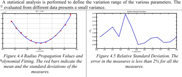
A statistical analysis is performed to define the variation range of the various parameters. The !! _{evaluated from different data presents a small variance.}

Figure 4.4 Radius Propagation Values and Polynomial Fitting. The red bars indicate the

mean and the standard deviations of the measures.

Figure 4.5 Relative Standard Deviation. The error in the measures is less than 2% for all the

measures.

The performed tests on the apparatus evidence the repeatability in the parameter evaluations. The curves from the data fitting present the expected parabola behaviors and the obtained values are consistent with the ones available in literature.

0 2 4 6 8 10 12 14 0 0.01 0.02 0.03 0.04 0.05 0.06 0.07 Cutoff Level mW /W m

Cutoff Level Influence on the Std

m_x m_y 0 5 10 15 20 25 30 35 40 45 50 62.4 62.6 62.8 63 63.2 63.4 63.6 63.8 64 64.2 64.4 Wx and W y [px] N° Picture Test of the Beam Radius Estimation

W_y W x 430 440 450 460 470 480 490 2 4 6 8 10 12 14 16x 10 ï3 M_x2 = 1.3215 1.3125 1.3171 1.3194 1.3263 zïAxis [mm] Wx 2 [µ m] 430 440 450 460 470 480 490 2 4 6 8 10 12 14 16x 10 ï3 Mx 2 = 1.3195 zïAxis [mm] Wx 2 [µ m] 435 440 445 450 455 460 465 470 475 480 485 0 0.002 0.004 0.006 0.008 0.01 0.012 0.014 0.016 0.018 zïAxis [mm] m /W m

Figure 4.6 Beam Section Image. Interference Fringes caused by dust grains generate

distortions in the image.

Figure 4.7 Dust grains produce the circular patterns. The diffraction caused by the ND filter

produces the straight lines.

In the hardware layout especially care must be observed in the cleaning of the optical elements. Dust grains and fingerprints must be eliminated from the transparent and reflective surfaces.

5.

OPTICAL SURFACE INSPECTION

Measurement of surface topography plays an important role in manufacturing, being used for both the control of manufacturing processes and for final product acceptance. A large number of devices based on optical phenomena have been developed for surface inspection, due to the fact that contactless instruments normally provide a faster and less invasive analysis. A recent review of these devices is available in (Hocken, Chakraborty, & Brown, 2005).

5.1 Laser Beam Reflection and Speckle Patterns

Illuminating a rough surface with a coherent light, a typical granular pattern characterizes the diffused light. This granularity is caused by scattering of the coherent illumination and the interference of the scattered light when an image is formed. Since the scattering is caused by the surface roughness the nature of the granularity, called speckle, can be used to deduce properties of the surface roughness. Many researchers have demonstrated a relation between the roughness parameter of metallic surfaces !_! and the correlation coefficients of the speckle images.

5.1.1 Specimens

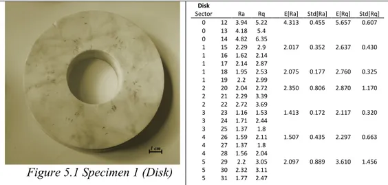
Figure 5.1 Specimen 1 (Disk)

Disk                  

Sector     Ra   Rq     E[Ra]   Std[Ra]   E[Rq]   Std[Rq]   0   12   3.94   5.22     4.313   0.455   5.657   0.607   0   13   4.18   5.4             0   14   4.82   6.35             1   15   2.29   2.9     2.017   0.352   2.637   0.430   1   16   1.62   2.14             1   17   2.14   2.87             1   18   1.95   2.53     2.075   0.177   2.760   0.325   1   19   2.2   2.99             2   20   2.04   2.72     2.350   0.806   2.870   1.170   2   21   2.29   3.39             2   22   2.72   3.69             3   23   1.16   1.53     1.413   0.172   2.117   0.320   3   24   1.71   2.44             3   25   1.37   1.8             4   26   1.59   2.11     1.507   0.435   2.297   0.663   4   27   1.37   1.8             4   28   1.56   2.04             5   29   2.2   3.05     2.097   0.889   3.610   1.456   5   30   2.32   3.11             5   31   1.77   2.47            

Two specimens of Carrara marble stone have been prepared with different surface roughness for the optical analysis. Several zones were grinded with Cardoso stone for different time to obtain various values of roughness. The zones have been then characterized with the MAHR Perthometer S3P roughness tester, measuring the roughness parameters.

5.1.2 Experimental Setup

The employed laser source was a !"#" laser, ! = 5  !", ! = 632.8  !" from Melles Griot. The images were collected with the digital camera Canon EOS 350D. On the camera was mounted the Canon MP-E 65mm 1-5x Macro Lens. The zoom was 4x, the camera recorded the images in the specular direction. Both the camera and the laser were at 60° form the normal of the specimen surface. The camera was set in manual mode, with iris aperture !16 and exposure time 1/800.

5.1.3 Image Analysis

Figure 5.2 Speckle Pattern in a Laser Image obtained from the Disk.

Figure 5.3 Picture of the Illuminated Surface in Figure 5.2

The collected images are analyzed with the algorithms proposed in (Dhanasekar, Krishna Mohan, Bhaduri, & Ramamoorthy, 2008) and (Pino, Pladellorens, Cusola, & Caum, 2011), developed for metallic surfaces.

The images are first cropped around the barycenter with a rectangular mask, and then the autocorrelation matrix is calculated. From this matrix the integrated correlation coefficient is

evaluated and related to the zone roughness, see Figure 5.4. The averaged intensity is calculated from the images and it is plotted against the roughness parameter !!, exposed in Figure 5.5.

5.2 Results

The two indicators extracted from the images present regions with a possible correlation with the surface roughness. However, the wideness of the deviation between values from the same roughness region suggests that the proposed methods, firstly employed on metallic surfaces, are not sufficiently accurate for stone surface inspections.

Figure 5.4 Integrated Autocorrelation

Function versus the !_! parameter. Three images

are analyzed at each roughness level. The red stars represent the relative IAF values. The bars

are the standard deviations from these values. The solid line connects the mean values.

Figure 5.5 Averaged Intensity of the Images

versus the !_! parameter. The symbols are the

same. The graph shows an interesting behavior

for roughness levels of 4 ÷ 6  !".

1 2 3 4 5 6 7 8 0.49 0.5 0.51 0.52 0.53 0.54 0.55 0.56 0.57 0.58 0.59

Integrated Autocorrelation against R_a

R_q [!m] Y AutoC 1 2 3 4 5 6 7 8 12 14 16 18 20 22 24 26 28 30

Mean Intensity against R_a

R_q [!m]

Y

6.

CONCLUSIONS

The design and the realization of a !! _{measurement apparatus have been discussed. The device}

can characterize the geometrical parameters of low power lasers, like those used in measure instruments, in the range of ! = 500 ÷ 1000  !" and !_! = 0.8 ÷ 2.5  !!.

The hardware design offers an improvement to the previous layouts for the !! _{estimation. Using a}

prism instead of two mirrors permits saving space in the orthogonal direction to the beam path. Actually the measurement requires at least 20 minutes. The movement of the prism is precise when the position is modified using the micrometric drive but is affected by a systematic error after the stage translation. In the graphs a data shift due to a misreading on the ruler is quite evident.

These problems could be solved introducing a motorized rail guide with integrated position read out. Considering 3 seconds to autoset the exposure time and take the pictures for a determined position and 1 second to modify the stage displacement, a complete acquisition of 25 ÷ 30 images would take less than 2 minutes. Commercial translation stages are quite expensive; an ad-hoc solution for this apparatus would be preferable.

A technique used on metallic surface to estimate the superficial roughness has been tested in the characterization of Carrara marble stones. Despite some agreements with the measured roughness, the method results not accurate as in the metallic surface control.

Undergraduate students will use the apparatus in laboratory experiments at the University of Erlangen-Nürnberg to understand and comprehend the laser propagation behavior.

REFERENCES

[1]. Alda, J. (2003). Laser and Gaussian Beam Propagation and Transformation. In R. G. Diggers, Encylopedia of

Optical Engineering (pp. 999-1013). Marcel Dekker.

[2]. Alsultanny, Y. A. (2006). Laser Beam Analysis Using Image Processing. Journal of Computer Science 2 , 109-113.

[3]. Andrews, J. T., Gupta, B. K., Bose, K., & Kumar, A. (2007). Low Cost Undergraduate Experiments with Lasers and

Personal Computer. Wseas Transactions on Advances in Engineering Education , 155-157.

[4]. Dhanasekar, B., Krishna Mohan, N., Bhaduri, B., & Ramamoorthy, B. (2008). Autocorrelation analysis of spectral

dependency of surface roughness speckle patterns. Precision Engineering , 32, 196–206.

[5]. Dicrks, F. (2004). Sensitivity and Image Quality of Digital Cameras. Basler Vision Technologies.

[6]. Hocken, R. J., Chakraborty, N., & Brown, C. (2005). Optical Metrology of Surfaces. CIRP Annals - Manufacturing

Technology , 169–183.

[7]. Micron. (2010). MT9M001 Megapixel CMOS Digital Image Sensor. Micron.

[8]. National Instruments. (2009). Labview 2009 User Manual. National Instruments.

[9]. Paschotta, R. (2011, 1 12). Encyclopedia for Photonics and Laser Technology. Retrieved 12 9, 2011, from RP

Photonics: http://www.rp-photonics.com/encyclopedia.html

[10]. Pedrotti, F. L. (1993). Introduction to Optics. Engelwood Cliffs: Prentice-Hall International Inc.

[11]. Pino, A., Pladellorens, J., Cusola, O., & Caum, J. (2011). Roughness Measurement of Paper using Speckle. Optical

Engineering , 50 (9), 562-568.

[12]. Roundy, C. B. (2005). Current Technology of Beam Profile Measurements. Logan (UT): Spiricon, Inc.

[13]. Savechenko, E. V. (2003). Determination of Coordinates of the Center of a Gaussian Beam. Measurement

Techniques , 46 (12), 99-104.

[14]. Schweinsberg, A., & Van Woerkom, L. (1999). Development of a Method for Measuring the M2 Parameter of a

Laser. Cornell University, Columbus (OH).

[15]. Self, S. A. (1983, March 1). Focusing of Spherical Gaussian Beams. Applied Optics , 20 (5), pp. 658-661.

[16]. Siegman, A. E. (1993). Defining, measuring, and optimizing laser beam quality. SPIE 1688 , 2, 1-11.

[17]. Siegman, A. E., & Ginzton, E. L. (1997). How to (Maybe) Measure Laser Beam Quality. Optical Society of America

Annual Meeting. Long Beach (CA).

[18]. Thorlabs. (2010). DCU22x and DCC1x45 Series User Manual. Thorlabs.

[19]. Thorlabs, Inc. (2011, 12 1). Thorlabs Product. Retrieved from Thorlabs: www.thorlabs.com

[20]. Xuezeng, Z., & Zhao, G. (2009). Surface roughness measurement using spatial-average analysis of objective speckle