Synthesis and Physico-Chemical characterization of anion-exchange polymeric materials for electrochemical applications

(1)

U

NIVERSITÀ DEGLI

S

TUDI DI

P

ISA

F

ACOLTÀ DI

S

CIENZE

M

ATEMATICHE

,

F

ISICHE E

N

ATURALI

D

OTTORATO DI

R

ICERCA IN

S

CIENZE

C

HIMICHE

XXIII

CICLO

SSD

CHIM/05

Synthesis and Physico-Chemical characterization of

anion-exchange polymeric materials for

electrochemical applications

Ph.D. Thesis

S

UBMITTED BY

Antonio Filpi

S

UPERVISOR

Prof. Francesco Ciardelli

E

XTERNAL

E

XAMINER

Prof. Hubert Gasteiger

(2)

First of all, I would like to thank my thesis supervisor, Prof. Francesco Ciardelli, for his warm encouragement and thoughtful guidance throughout my doctoral studies.

I would like to sincerely thank Acta S.p.A. for their financial support and all the instrumentation provided for electrochemical characterization. I am especially grateful to all the people that worked with me in ACTA, who have assisted and encouraged me in various ways during my research.

My thanks to Tokuyama Corp. for providing their commercial anion-exchange materials. My thanks to Dr. Andrea Pucci for his support and precious advices. I want to express my gratitude to all the people working in the research group of the University of Pisa for their precious collaboration on the membrane synthesis.

My thanks to Dr. Hubert Gasteiger for giving me the opportunity to start my Ph.D. and reviewing my dissertation. His ideas and tremendous support during the early stages of this research had a major influence on this thesis.

The writing of a dissertation is obviously not possible without the personal and practical support of numerous people. Thus my sincere gratitude goes to all my friends for their support and patience over the last few years.

Last but not least, I wish to thank my family who have always supported me in all the choices I've made throughout my life.

(3)

Summary

In the last few years a number of new anion-exchange polymers have been developed, offering the possibility of assembling Membrane Electrode Assemblies (MEAs) to develop Anion-exchange Membrane Fuel Cells (AMFCs) and Anion-exchange Membrane-based Electrolyzers (AMEs).

The current technologies of Anion Exchange Materials (AMs) for electrochemical application shows several limitations relate to the possibility of obtaining a reasonable low cost membrane having: high ionic conductivity, chemical stability in strong alkaline media, low permeability, low water swelling and good mechanical properties.

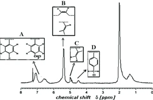
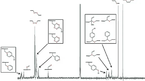
The purpose of this study was to develop and characterize AMs based on Styrene– butadiene–styrene (SBS) copolymer, a thermoplastic material with a block structure widely employed in the rubber industry. In the present work is reported a controlled radical functionalization, initiated by benzoyl peroxide (BPO), of SBS with 4-vinylbenzyl chloride (VBC). The resulting thermoplastic polymer was converted into an anion exchange membrane via quaternization reaction with aliphatic amines, such as trimethylamine or 1,4-diazabicyclo[2.2.2]octane (DABCO). Electrochemical properties of these materials were measured and correlated with synthetic parameters. Correlations between transport properties and synthetic parameters were explained in terms of Cluster-Network morphological model. Performance of the synthesized SBS-based AMs were then evaluated in a working AMFC and compared with commercial materials. Diagnostics on AMFCs, by means of electrochemical impedance spectroscopy (EIS), were performed in order to evaluate measured performances.

(4)

1 _Introduction

Proton Exchange Membrane Fuel Cells (PEMFCs) and Proton Exchange Membrane Electrolyzers (PEM-E) have been developed over the last 20 years, however high loading of precious metal catalysts on the oxygen reduction (PEMFC)/oxygen evolution (PEM-E) side is still required due to the slow kinetics of the oxygen reduction reaction (ORR) (1) and oxygen evolution reaction (OER) (2).

Alkaline environment enable usage of first row transition metal based catalysts which are intrinsically stable and have an activity similar to platinum. A major issue related to traditional aqueous electrolyte alkaline fuel cells was the presence of mobile cations (e.g. K+_, Na+_{) which could precipitate as carbonate that block or destroy the catalyst layers (3). Using} ionomer bound MEAs (Membrane Electrode Assemblies), analogous to PEMFCs, the carbonate precipitation issue would be overcome. In fact, the cationic sites (typically quaternary ammonium sites) are grafted and immobilised on the skeleton of the polymer chain. In strong alkaline environment quaternary ammonium sites degradation occurs via two different mechanisms: Hoffmann elimination and/or methyl and ammine direct nucleophilic displacement by hydroxide ions. Recent studies have demonstrated that the stability of ammonium sites towards alkali, can be increased by polymer crosslinking using a diamine (4).

In the last few years a number of new anion-exchange polymers (5; 6; 7; 8; 9; 10; 11; 12; 13; 14) have been developed, offering the possibility of assembling MEAs to develop Anion-exchange Membrane Fuel Cells (AMFCs) and Anion-Anion-exchange Membrane-based Electrolyzers (AMEs).

The current technologies of Anion Exchange Materials (AMs) for electrochemical application shows several limitations relate to the possibility of obtaining a reasonable low cost membrane having: high ionic conductivity, chemical stability in strong alkaline media, low permeability, low water swelling and good mechanical properties.

It has been recently discovered that the hydrogen oxidation reaction (HOR)/hydrogen evolution reaction (HER) kinetics on platinum catalyst are several orders of magnitude slower in alkaline compared to acid electrolyte (15). Therefore, the use of platinum anode catalysts in AMFCs/AMEs would require high loadings and thus become a significant cost factor unlike in PEMFCs/PEM-Es, where low Pt anode loadings are sufficient.

However transition metals oxide based catalysts, particularly spinel-type structures and transition metals alloys have been considered most promising for OER and HER (16; 17; 18; 19). Moreover other non-noble metal-based catalysts are available for AMFCs with an ORR activity comparable to Pt/C (20).

Therefore, the development of highly efficient catalysts toward HOR in alkaline electrolyte and cheap AMs having high conductivity and low water swelling are the critical challenges to make AMFCs/AMEs more practical.

The purpose of this study was to develop and characterize an AM based on Styrene– butadiene–styrene copolymer (SBS), a thermoplastic material with a block structure widely

(7)

employed in the rubber industry. It is well known how to introduce functional groups by radical grafting in SBS copolymer (21; 22; 23). In the present work is reported a controlled radical functionalization, initiated by benzoyl peroxide (BPO), of SBS with 4-vinylbenzyl chloride (VBC). The resulting thermoplastic polymer was converted into an anion exchange membrane via quaternization reaction with aliphatic amines, such as trimethylamine or 1,4-diazabicyclo[2.2.2]octane (DABCO), in the form of a thin sheet (50-100 µm).

The final properties of these SBS-based AMs will be reported in terms of ion-exchange capacity (IEC), ionic conductivity (σ), water uptake (WU). Commercial materials will be also evaluated and used as benchmarks.

The relationship between ion-exchange material structure and transport properties, such as ionic conductivity, is a critical driving force for much of the structural research on ion-exchange materials and provides the foundation for fundamental modeling work on these materials. Cluster-Network morphology model is widely used to describe the fundamental relationship between ionomer structure and electrochemical properties (24). Correlations between transport properties and synthetic parameters will be thus explained in terms of Cluster-Network morphological parameters.

Performance of the obtained SBS-based materials will be then evaluated in a working AMFC and compared with commercial AMs. Diagnostics on AMFCs, by means of electrochemical impedance spectroscopy (EIS), will be then performed in order to determine performance loss sources.

(8)

1.1 _{Electrochemistry}

Electrochemistry is a branch of chemistry that studies chemical reactions which take place in a solution at the interface of an electron conductor (a metal or a semiconductor) and an ionic conductor (the electrolyte), and which involve electron transfer between the electrode and the electrolyte or species in solution.

If a chemical reaction is driven by an external applied voltage, as in electrolysis, or if a voltage is created by a chemical reaction as in a battery, it is an electrochemical reaction. In contrast, chemical reactions where electrons are transferred between molecules are called oxidation/reduction (redox) reactions. In general, electrochemistry deals with situations where oxidation and reduction reactions are separated in space, connected by an external electric circuit.

An electrochemical cell consists of two electrodes, or metallic conductors, in contact with an electrolyte, an ionic conductor (which may be a solution, a liquid, or a solid). An electrode and its electrolyte comprise an electrode compartment. The two electrodes may share the same compartment. The various kinds of electrode are summarized in Table 1. Any 'inert metal' shown as part of the specification is present to act as a source or sink of electrons, but takes no other part in the reaction other than acting as a catalyst for it. If the electrolytes are different, the two compartments may be joined by a salt bridge, which is a tube containing a concentrated electrolyte solution (almost always potassium chloride in agar jelly) that completes the electrical circuit and enables the cell to function. A galvanic cell is an electrochemical cell that produces electricity as a result of the spontaneous reaction occurring inside it. An electrolytic cell is an electrochemical cell in which a non-spontaneous reaction is driven by an external source of current.

Electrode type Designation Redox couple Half-reaction Metal/metal ion M(s) I M+_(aq) _M+_/M _M+_{(aq) + e}-_{→ M(s)} Gas Pt(s) I X2(g) I X+(aq) X+/X2 X+(aq) + e- → X2(g)

Pt(s) I X2(g) I X-(aq) X2/X- X2(g) + 2e- →2X-(aq) Metal/insoluble salt M(s) I MX(s) I X-_(aq) _MX/M,X- _{MX(s) +e}-_{→ M(s) + X}-_(aq) Redox Pt(s) I M+_(aq),M2+_(aq) _M2+_/M+ _M2+_{(aq) + e}-_{→ M}+_(aq)

Table 1. Varieties of electrode

The reduction and oxidation processes responsible for the overall reaction in a cell are separated in space: oxidation takes place at one electrode and reduction takes place at the other. As the reaction proceeds, the electrons released in the oxidation Red1 → Ox1 + ν e- at one electrode travel through the external circuit and re-enter the cell through the other electrode. There they bring about reduction Ox2 + ν e- → Red2. The electrode at which oxidation occurs is called the anode; the electrode at which reduction occurs is called the cathode. In a galvanic cell, the cathode has a higher potential than the anode: the species undergoing reduction, Ox2, withdraws electrons from its electrode (the cathode), so leaving a relative positive charge on it (corresponding to a high potential). At the anode, oxidation

(9)

results in the transfer of electrons to the electrode, so giving it a relative negative charge (corresponding to a low potential).

1.1.1 _{Thermodynamics}

The fundamental equation for a multicomponent system establishes:

𝑑𝑈 = 𝑇𝑑𝑆 − 𝑃𝑑𝑉 + � 𝜇𝑖𝑑𝑛𝑖 𝑖

(1.1)

where U is the internal energy, V the volume, S the entropy, T the temperature in Kelvin, µi is the chemical potential of the species i and ni is the number of moles of the species i. The

chemical potential µi is defined as the change in molar internal energy with the number of

moles ni of the species i at constant volume and entropy (i.e. isochoric and adiabatic

process):

𝜇𝑖 = �_𝜕𝑛𝜕𝑈

𝑖�𝑆,𝑉,𝑛𝑗≠𝑖

(1.2)

Gibbs free energy G is defined as:

𝐺 = 𝑈 + 𝑃𝑉 − 𝑇𝑆 (1.3)

Differentiating equation (1.3) and combining it with equation (1.1) we obtain another form of the fundamental equation:

𝑑𝐺 = 𝑉𝑑𝑃 − 𝑆𝑑𝑇 + � 𝜇𝑖𝑑𝑛𝑖 𝑖

(1.4)

Thus, the chemical potential µi can be regarded as the reversible work for transferring

one mole of i from vacuum to a given phase at constant pressure and temperature:

𝜇𝑖 = �_𝜕𝑛𝜕𝐺

𝑖�𝑇,𝑃,𝑛𝑗≠𝑖

(1.5)

Euler’s theorem states that if we have a function F which is homogeneous of degree 1, i.e. F({αyi})=αF({yi}), then we can express it as the sum of its arguments weighted by the first partial derivatives:

𝐹({𝑦𝑖}) = � 𝑦𝑗�_𝜕𝑦𝜕𝐹 𝑗�_𝑦_𝑖≠𝑗 𝑗

(1.6)

Since internal energy U is homogeneous in all its arguments (entropy, volume and number of moles) we obtain:

𝑈 = 𝑇𝑆 − 𝑃𝑉 + � 𝜇𝑖𝑛𝑖 𝑖

(1.7)

Combining equations (1.7) and (1.3) we obtain for the free energy:

𝐺 = � 𝜇𝑖𝑛𝑖 𝑖

(1.8)

which differentiated and combined with equation (1.4) gives the Gibbs-Duhem equation:

� 𝑛𝑗𝑑𝜇𝑗 𝑗

= −𝑆𝑑𝑇 + 𝑉𝑑𝑃 _(1.9)

This equation shows that in thermodynamics intensive properties are not independent but related, making it a mathematical statement of the state postulate. When pressure and

(10)

potential and Gibbs' phase rule follows.

Partial derivative of equation (1.9) with respect to ni gives

𝑑𝜇𝑖 = 𝑉� 𝑑𝑃 𝚤 (1.10)

where 𝑉�� is the partial molar volume for component i. Applying Raoult’s law for ideal solutions 𝑖

and integrating equation (1.10) we obtain:

𝜇𝑖 = 𝜇𝑖0+ 𝑅𝑇 ln (𝑥𝑖) (1.11)

where 𝜇_𝑖0_{is the chemical potential of component i at standard conditions and x}_i_{is its}

molar fraction. Many pairs of liquids present no uniformity of attractive forces, i.e. the adhesive and cohesive forces of attraction are not uniform between the two liquids, so that they show deviation from the Raoult's law which is applied only to ideal solutions. For real solutions we have to take in account this deviations introducing in the “active” concentration or activity ai:

𝑎𝑖 = 𝛾𝑖𝑐𝑖 (1.12)

where 𝛾𝑖is the activity coefficient. Substituting the molar fraction with the activity in

equation (1.12) we obtain for real solutions:

𝜇𝑖 = 𝜇𝑖0+ 𝑅𝑇 ln (𝛾𝑖𝑐𝑖) (1.13)

Ion activities and Debye-Hückel theory

For a generic salt MnXm:

𝐺 = 𝑛 𝜇++ 𝑚 𝜇−= 𝐺𝑖𝑑𝑒𝑎𝑙+ 𝑅𝑇 ln[(𝛾+)𝑛(𝛾−)𝑚] (1.14) It is convenient to introduce the mean activity coefficient 𝛾±:

𝛾±= [(𝛾+)𝑛(𝛾−)𝑚] 1

𝑛+𝑚 (1.15)

Peter Debye and Erich Hückel proposed a model (25) in 1923 for calculating the activity coefficient arguing that the energy of an ion is lowered by electrostatic interactions with its ionic atmosphere. Their main assumptions were:

 Interactions are primarily columbic;

 Electrolyte is fully dissociated at all concentrations;

 Permittivity of the electrolyte is equal to the one of the pure solvent;  Ions are rigid charged spheres (non-polarisable);

 Electrostatic interaction is smaller than kBT (where kB is the Boltzmann constant); The final result yields the so-called extended Debye- Hückel equation:

𝐿𝑜𝑔 𝛾±= 𝑧+𝑧− 𝐴√𝐼

1 + 𝑎±𝐵√𝐼

(1.16)

where z is the integer charge of the ions, a± is the effective hydrated radius of the ions, I is the ionic strength of the solution, A and B are constants with values of respectively 0.5085 and 0.3281 at 25°C in water (26). For diluted solutions (I≤10-4M) equation (1.16) can be reduced to the Debye-Hückel limiting law:

(11)

Electrostatic potential of condensed phases

The electrostatic inner potential φ, also known as Galvani potential, determines the reversible work for transferring a positive charge unit from vacuum to the interior of the condensed phase:

𝜙 = 𝜓 + 𝜒 (1.18)

where ψ is the outer or Volta potential, determined by the distance separating the unit charge form the plane of closest approach to the phase and χ is the surface potential, related to the differential work for bringing the charge to the interior of the phase.

Figure 1. Diagram for a charged condensed phase having a spherical geometry

Assuming a spherical geometry (Figure 1) we obtain the following equation for the inner potential:

𝜙 =_{4𝜋𝜖𝜖} 𝑞

0(𝑥 + 𝑟) + 𝜒 (1.19)

Electrochemical potential of charged species

The electrochemical potential 𝜇� is defined as the sum of chemical and electrostatic 𝚤

potential for a mole of the i-th compound having charge zi:

𝜇�_𝑖 = 𝜇_𝑖+ 𝑧𝑖𝐹𝜙 (1.20)

where F is the Faraday constant, equal to the magnitude of electric charge per mole of electrons. On Figure 2 are sketched contributions to the electrochemical potentials.

Figure 2. Contributions to the electrochemical potential Combining equations (1.20) and (1.13) we obtain:

𝜇�_𝑖= 𝜇_𝑖0_{+ 𝑅𝑇𝑙𝑛 (𝛾}

𝑖𝑐𝑖) + 𝑧𝑖𝐹𝜙 (1.21)

Equilibrium and the Galvani potential difference

For a general chemical process:

𝛼𝐴(𝑎𝑞)+ 𝛽𝐵(𝑎𝑞)⇌ 𝛿𝐷(𝑎𝑞) (1.22)

Gibbs free energy variation comes from equation (1.4):

(12)

Since the process is isobaric and isothermal 𝑉𝑑𝑃 and 𝑆𝑑𝑇 terms are null. Moreover from balance of matter, introducing stoichiometric coefficients 𝜈𝑖, moles variations 𝑑𝑛𝑖 should be

equal to:

𝑑𝑛𝑖 = 𝜈𝑖𝑑𝜉 (1.24)

where 𝜉 is the extent of reaction or reaction coordinate. Combining equations (1.23) (1.24) and (1.13) we obtain: 𝑑𝐺 = �𝛿𝜇𝐷0 − 𝛼𝜇𝐴0− 𝛽𝜇𝐵0+ 𝑅𝑇 �ln � 𝑐𝐷 𝛿 𝑐_𝐴𝛼_𝑐 𝐵𝛽 𝛾𝐷𝛿 𝛾_𝐴𝛼_𝛾 𝐵𝛽 �� 𝑑𝜉 (1.25)

Defining the reaction Gibbs free energy Δ𝑟𝐺𝑇,𝑃 as:

Δ𝑟𝐺𝑇,𝑃= �𝜕𝐺_{𝜕ξ �} 𝑇,𝑃

(1.26)

the reaction quotient 𝑄𝑟 as:

𝑄𝑟 = ∏ 𝑎_𝑝𝜈𝑝 𝑝 ∏ 𝑎_𝑟𝜈𝑟 𝑟 (1.27)

where indexes 𝑝 and 𝑟 refers respectively to products and reagents, and Gibbs free energy at standard conditions Δ𝑟𝐺𝑇,𝑃0 as:

Δ𝑟𝐺𝑇,𝑃0 = � 𝜈𝑖𝜇𝑖0 𝑖

(1.28)

equation (1.25) can be rearranged as:

Δ𝑟𝐺𝑇,𝑃 = Δ𝑟𝐺𝑇,𝑃0 + 𝑅𝑇 ln 𝑄𝑟 (1.29)

known as Van’t Hoff isotherm.

At the equilibrium 𝑑𝐺 = 0 or equivalently Δ𝑟𝐺𝑇,𝑃 = 0 ⟺ ln 𝑄𝑟 = −Δ𝑟𝐺𝑇,𝑃 0

𝑅𝑇 , hence the

reaction quotient has to be constant, known as equilibrium constant 𝐾:

𝐾 = 𝑒−Δ𝑟𝐺𝑇,𝑃

0

𝑅𝑇 (1.30)

Similarly for an electrochemical process:

𝑂𝑥(𝑎𝑞)+ 𝑛 𝑒(𝑀)− ⇌ 𝑅𝑒𝑑(𝑎𝑞) (1.31)

Gibbs free energy variation is:

𝑑𝐺� = 𝜇�𝑟𝑒𝑑𝑑𝑛𝑟𝑒𝑑 + 𝜇�𝑜𝑥𝑑𝑛𝑜𝑥+ 𝜇�𝑒𝑑𝑛𝑒 + 𝑉𝑑𝑃 − 𝑆𝑑𝑇 (1.32) which rearranged and combined with equation (1.21) gives the electrochemical reaction free energy Δ𝑟𝐺�𝑇,𝑃: Δ𝑟𝐺�𝑇,𝑃= Δ𝑟𝐺�𝑇,𝑃0 + 𝑅𝑇 ln𝑎_𝑎𝑟𝑒𝑑 𝑜𝑥 + 𝑛𝐹Δ𝑎𝑞 𝑀 _ϕ _(1.33) where Δ𝑀𝑎𝑞ϕ = ϕM− ϕaq and Δ𝑟𝐺�𝑇,𝑃0 = 𝜇𝑜𝑥0 (𝑎𝑞) − 𝜇𝑟𝑒𝑑0 (𝑎𝑞) + 𝑛 𝜇𝑒(𝑀) At the equilibrium Δ𝑟𝐺�𝑇,𝑃 = 0: Δ𝑀𝑎𝑞ϕ = Δ𝑀𝑎𝑞ϕ0−RT_{nF ln}a_ared ox (1.34)

(13)

where:

Δ𝑀𝑎𝑞ϕ0=Δ𝑟𝐺�𝑇,𝑃 0

𝑛𝐹 (1.35)

equation (1.34) describes a unique relationship between the Galvani potential difference and the activity ratio of the redox species. On Figure 3 Galvani potential difference is reported for different electrode types.

Figure 3. Galvani potential difference relationships for different electrode types

The cell potential and the electromotive force

By definition, the cell potential corresponds:

𝐸𝑐𝑒𝑙𝑙= Δ𝑀𝑎𝑞ϕ(cathode) − Δ𝑎𝑞𝑀 ϕ(anode) (1.36) which combined with equation (1.34) and rearranged gives the Nernst equation:

𝐸𝑐𝑒𝑙𝑙= 𝐸𝑐𝑒𝑙𝑙0 −𝑅𝑇_{𝑛𝐹 ln 𝑄} (1.37) where 𝐸_{𝑐𝑒𝑙𝑙}0 _{= Δ} 𝑎𝑞 𝑀 _ϕ0_{(cathode) − Δ} 𝑎𝑞 𝑀 _ϕ0_(anode) _(1.38)

A cell in which the overall cell reaction is not at the equilibrium can generate electrical work. The cell potential is directly related to the magnitude of this work. In this respect, the 𝐸𝑐𝑒𝑙𝑙 is also known as the electromotive force. It follows:

(14)

Figure 4. Gibbs free energy as a function of the extent of the reaction

The minimum in the curve reported in Figure 4 corresponds to the equilibrium state. As the Gibbs free energy of the cell reaction is zero, the cell cannot perform any external work. Consequently at equilibrium 𝑄 = 𝐾, equilibrium constant of the cell reaction:

ln 𝐾 =𝑛𝐹𝐸_𝑅𝑇𝑐𝑒𝑙𝑙0 (1.40)

Moreover from equation (1.39):

𝐸_{𝑐𝑒𝑙𝑙}0 _{= −}Δ𝑟𝐺�𝑇,𝑃0

𝑛𝐹 (1.41)

Standard potentials

The cell potential is determined by the potentials at the cathode and anode. 𝐸𝑐𝑒𝑙𝑙 can be

measured accurately, however, the potential at each individual electrode cannot be measured. A convention is needed:

𝐻_(𝑎𝑞)+ + 𝑒_(𝑀)− _{→ 1 2}� 𝐻2(𝑔)

Δ𝑀𝑎𝑞𝜙 = Δ𝑀𝑎𝑞𝜙0−𝑅𝑇_{𝐹 ln}_𝑎1 𝐻+

Δ𝑀𝑎𝑞𝜙0= 0

(1.42)

This means the half cell Pt(s)|H2(g)|H+(aH+=1,aq) has a Galvani potential equal to zero at all temperature. On the basis of this assumption, the standard potential for half cell reactions can be estimated by means of Bordwell thermodynamic cycles.

Temperature effects

By using the basic relation between the cell potential and the Gibbs free energy change in equation (1.39), it follows that:

�𝜕𝐸_{𝜕𝑇 �}𝑐𝑒𝑙𝑙 𝑃= − 1 𝑛𝐹 � 𝜕Δ𝑟𝐺� 𝜕𝑇 �_𝑃= Δ𝑟𝑆̃ 𝑛𝐹 (1.43)

If we assume that Δ𝑟𝑆� is independent of temperature (i.e., Δ𝑟𝐶𝑃 is small), we can

integrate equation (1.43), to give:

𝐸𝑐𝑒𝑙𝑙(𝑇) = 𝐸𝑐𝑒𝑙𝑙(𝑇0) +Δ_{𝑛𝐹 (𝑇 − 𝑇}𝑟𝑆̃ 0) (1.44) Note that for many redox reactions Δ𝑟𝑆� is small (less than 50 J/K). This leads to only

(15)

10-5_{- 10}-4_{V/K change in 𝐸}

𝑐𝑒𝑙𝑙; hence, the cell potential is relatively insensitive to

temperature. Finally, by noting that at constant temperature, Δ𝐻 = Δ𝐺 + 𝑇Δ𝑆, and using equation (1.43), we see that

�𝜕 𝐸 𝑐𝑒𝑙𝑙 𝑅𝑇 𝜕𝑇 � = Δ𝑟𝐻� 𝑛𝐹𝑅𝑇2 (1.45)

which is basically the Gibbs-Helmholtz equation for electrochemical equilibrium.

1.1.2 _{Transport of species in solution}

Mass transport in electrolyte solution can be induced by three processes: _Convection



– mechanical or thermal agitation; Migration



– gradient of an electrical field (ions); Diffusion

Neglecting convection forces and recalling the concept of electrochemical potential of anion i (𝜇� ): 𝚤

– gradient of chemical potential.

𝜇�_𝑖 = 𝜇_𝑖0_{+ 𝑅𝑇𝑙𝑛 (𝑎} 𝑖) �� Diffusion + 𝑧�𝑖𝐹𝜙 Migration (1.46)

Conductivity of electrolyte solutions

Ions in solution can be set in motion by applying a potential difference between two electrodes. The conductance Λ of a solution is defined as the inverse of the electric resistance 𝑅:

Λ =_𝑅1 (1.47)

The SI unit of conductance is the siemens (S): 1𝑆 = 1/Ω. For parallel plate electrodes with area 𝐴, at the distance 𝑙 it follows:

Λ = 𝜒𝐴_𝑙 (1.48)

where 𝜒 is the conductivity, expressed in S/m. The electrical conductivity of a solution of an electrolyte is measured by determining the resistance of the solution between two flat or cylindrical electrodes separated by a fixed distance (27). An alternating voltage is used in order to avoid electrolysis. The resistance is measured by a conductivity meter. Typical frequencies used are in the range 1-3 kHz. The dependence on the frequency is usually small (28), but may become appreciable at very high frequencies, an effect known as the Debye– Falkenhagen effect. The conductivity of a solution depends on the number of ions present. Consequently, the molar conductivity Λ𝑚 is used:

Λm=𝜒_𝑐 (1.49)

where 𝑐 is the electrolyte molar concentration. In real solutions, Λ𝑚 depends on the

concentration of the electrolyte. This could be due to: _{Ion-ion interactions: 𝛾}_± _{≠ 1;}

(16)

conductivity of a large quantity of strong electrolytes. These results led to the Kohlrausch law:

Λ𝑚 = Λ0𝑚− 𝐾√𝑐 (1.50)

where Λ0𝑚is known as the limiting molar conductivity, K is an empirical constant and c is

the electrolyte concentration. Moreover, Kohlrausch also found that in the limit of zero concentration, as ion-ion interactions are negligible, it can be postulated that the limiting conductivity of anions and cations are additive, i.e. the conductivity of a solution of a salt is equal to the sum of conductivity contributions from the cation and anion:

Λ0𝑚 = 𝜈+𝜆+0 + 𝜈−𝜆−0 (1.51)

where 𝜆+0 and 𝜆−0 are the limiting molar conductivity of the cation and anion,

respectively, 𝜈+ and 𝜈− are the numbers of cations and anions per formula unit of

electrolyte. Equation (1.51) is known as “Law of independent migration of ions”. Debye and Hückel modified their theory in 1926 and their theory was further modified by Lars Onsager in 1927. All the postulates of the original theory were retained. In addition it was assumed that the electric field causes the charge cloud to be distorted away from spherical symmetry. After taking this into account, together with the specific requirements of moving ions, such as viscosity and electrophoretic effects, Onsager was able to derive a theoretical expression to account for the empirical Kohlrausch's Law.

A weak electrolyte is one that is not fully dissociated . Typical weak electrolytes are weak acids and weak bases. The concentration of ions in a solution of a weak electrolyte is less than the concentration of the electrolyte itself. For acids and bases the concentrations can be calculated when taking in account for the degree of dissociation 𝛼:

Λ𝑚 = 𝛼Λ0𝑚 (1.52)

For a monoprotic acid, HA, with a dissociation constant Ka, an explicit expression for the conductivity as a function of concentration, c, known as Ostwald's dilution law, can be obtained from equation (1.52):

1 Λ𝑚 = 1 Λ0𝑚+ Λ𝑚𝑐 𝐾𝑎(Λ0𝑚)2 (1.53)

Figure 5. Concentration dependence of the molar conductivities of a typical strong electrolyte (aqueous

(17)

On Figure 5 is reported the concentration dependence of molar conductivity of a typical strong and weak electrolytes.

The mobility of ions

Ion movement in solution is random. However, a migrating flow can be onset upon applying an electric field 𝐸�⃗:

�𝐸�⃗� =Δ𝜙_𝑙 (1.54)

where Δ𝜙 is the potential difference between two electrodes separated by a distance 𝑙. An ion of charge 𝑧𝑒−_{experiences a force 𝐹⃗:}

�𝐹⃗� = 𝑧 𝑒 �𝐸�⃗� =𝑧 𝑒 Δ𝜙_𝑙 (1.55)

𝐹⃗ accelerates cations to the negatively charged electrode and anions in the opposite direction. Through this motion, ions experience a frictional force in the opposite direction. Taking the expression derived by Stoke relating friction 𝐹𝑓𝑟𝑖𝑐 and the viscosity of the solvent

𝜂:

𝐹𝑓𝑟𝑖𝑐 = 6𝜋 𝜂 𝑎 𝑣 (1.56)

where 𝑎 is the hydrodynamic radius of the ion and 𝑣 is the drift speed, when the accelerating and retarding forces balance each other, 𝑣 is defined by:

𝑣 =_{6𝜋 𝜂 𝑎}𝑧 𝑒 �𝐸�⃗� = 𝑢�𝐸�⃗� (1.57)

where 𝑢 is the mobility of the ion, defined as the velocity attained by an ion moving under unit electric field:

𝑢 = 𝑣

�𝐸�⃗�= 𝑧 𝑒

6𝜋 𝜂 𝑎 (1.58)

Finally it can be shown that:

𝜆 = 𝑧 𝑢 𝐹 (1.59)

and equation (1.51) can be rewritten as:

Λ0𝑚 = (𝑧+𝑢+𝜈++ 𝑧−𝑢−𝜈−)𝐹 (1.60)

Diffusion

Conventional electrochemical processes take place at the electrode surface, creating non homogeneous composition of the electrolyte solution. A key phenomenological relationship developed by Adolf Fick in 1855 relates the diffusive flux to the concentration field, by postulating that the flux goes from regions of high concentration to regions of low concentration, with a magnitude that is proportional to the concentration. For ideal mixtures:

𝐽𝑖 = −𝐷𝑖∇𝑐𝑖 (1.61)

where 𝐽_𝑖 is the diffusion flux expressed as �𝑚𝑜𝑙_𝑚2_𝑠� and 𝐷𝑖 is the diffusion coefficient, or

diffusivity, expressed as �𝑚_𝑠2�. In chemical systems other than ideal solutions or mixtures, the driving force for diffusion of each species is the gradient of chemical potential of this species:

(18)

𝐽𝑖 = − _{𝑅𝑇 ∇𝜇}𝑖 (1.62) The following mass balance can be used in order to predicts how diffusion causes the concentration field to change with time:

𝜕𝑐𝑖

𝜕𝑡 = −∇𝐽𝑖 = ∇(𝐷𝑖∇𝑐𝑖) (1.63)

Assuming the diffusion coefficient D to be a constant we obtain from equation (1.63):

𝜕𝑐𝑖

𝜕𝑡 = 𝐷𝑖∇2𝑐𝑖 (1.64)

which is analogous to the heat equation. The equilibration of the diffusion and friction forces allows establishing:

𝐷𝑖 =𝑢_𝑧𝑖𝑅𝑇

𝑖𝐹 (1.65)

known as Einstein equation. According to equation (1.65), typical diffusion coefficients are of the order of 10-9 m2·s-1. The fact that mobility is related to the frictional force and the diffusion coefficient allows establishing a further important expression:

𝐷𝑖 =_{6𝜋𝜂𝑎}𝑘𝑏𝑇

𝑖 (1.66)

known as Stoke-Einstein equation. Note that the ionic charge does not figure in equation (1.66). This means that the diffusion coefficient is independent of the ionic charge. Equation (1.66) is also valid for neutral molecules.

Nernst-Plank equation

Summing all contributions to mass transport in electrolyte solutions obtained before, we obtain for the flux 𝐽𝑖:

𝐽𝑖 = −𝐷��𝑖∇𝑐𝑖 Diffusion − 𝑢��𝑖∇𝜙 Migration + 𝑐�𝑖τ Convection (1.67) where 𝜏 is the rate with which a volume element moves in solution. Combining equations (1.65) and (1.67) we obtain the so-called Nernst–Planck equation:

𝐽𝑖= −𝐷𝑖∇𝑐𝑖−𝑧_{𝑅𝑇 𝐷}𝑖𝐹 𝑖ci∇𝜙 + 𝑐𝑖𝜏 (1.68)

1.1.3 _Kinetics

In order to grasp what is taking place in an electrochemical reaction, the concept of current and how the current changes when a stimulus is applied must be understood. Two types of current may flow in an electrochemical cell, faradic and non-faradic. All currents that are created by the reduction and/or oxidation of chemical species in the cell are termed faradaic currents. The current is equal to the change in charge with time, or:

𝑖 =𝜕𝑄_𝜕𝑡 (1.69)

where 𝑖 is the Faradic current, and 𝑄 is the charge given by Faraday’s law. Faraday’s law correlates the total charge passed through a cell to the amount of product 𝑁 expressed in moles:

(19)

where 𝐹 is the Faraday’s constant (𝐹 = 96485 𝐶 𝑚𝑜𝑙−1_{) and 𝑛 is the number of}

electrons transferred per molecule of product. All other current is deemed non-faradic in nature, and is directly related to Ohm’s law:

𝑖𝑛𝑓=Δ𝑉_𝑅

Ω (1.71)

where 𝑖𝑛𝑓 is the non-faradic current, Δ𝑉 the potential difference, 𝑅 is the ohmic

resistance. While the resistance is applicable when considering Ohm’s law in an electrical circuit, the application to an electrochemical cell requires the usage of impedance 𝑍, which includes elements of resistance and capacitance.

Chemical reactions can be either homogeneous or heterogeneous. The first type occurs in a single phase, and its rate is uniform everywhere in the volume where it occurs:

Rate [𝑚𝑜𝑙 𝑠−1_{] =}𝜕𝑁

𝜕𝑡 (1.72)

Heterogeneous reactions occur at the electrode-solution interface, and they are characteristic of electrochemistry. While the expression for the reaction rate is similar to equation (1.72), it depends upon the area of the electrode, 𝐴, or the area of the phase boundary where the reaction occurs:

Rate [𝑚𝑜𝑙 𝑠−1_𝑐𝑚−2_{] =} 𝑖

𝑛𝐹𝐴 = 𝑗

𝑛𝐹 (1.73)

where 𝑗 is the faradic current density. There are four major factors that govern the reaction rate and current at electrodes:

1. Mass transfer to the electrode surface; 2. Kinetics of the electron transfer; 3. Preceding and ensuing reactions; 4. Surface reactions (adsorption).

The slowest process will be the rate determining step.

(20)

𝑂 + 𝑛𝑒−_{⇌ 𝑅} _(1.74) This reaction may be considered as a set of equilibria involved in the migration of the reactant to the electrode, the reaction at the electrode and the migration of the product away from the electrode surface into the bulk of the solution (Figure 6). For this reaction to proceed, 𝑂 is required to move from the bulk solution near the electrode surface. This aspect of the mechanism is related to mass transfer and is governed by the Nernst–Planck equation (1.68). Mass transfer from the bulk solution towards the electrode surface could limit the rate of the reaction. When all of the processes leading to the reaction are fast, this leaves the electron transfer reaction as the limiting factor.

Near the electrode an electrochemical double-layer is formed (Figure 7): the first layer, or inner Helmholtz plane (IHP), comprises ions adsorbed directly onto the electrode due to a host of chemical interactions, the second layer, or outer Helmholtz plane (OHP) is composed of ions attracted to the surface charge via the coulomb force, electrically screening the first layer itself.

This double-layer works as an electrochemical capacitor having capacitance 𝐶𝑑. So the

measured current is the sum of the faradic and faradic (capacitive) one. The non-faradaic time constant for the electrode 𝜏 [𝑠] can be calculated by:

𝜏 = 𝑅𝑠𝐶𝑑 (1.75)

where 𝑅𝑠 is the solution resistance and 𝐶𝑑 is the double layer capacitance. The double layer

charging will be complete (95%) in a time frame equal to 3τ (29).

(21)

Reversibility

Reversibility is a key concept when dealing with electrochemical reaction mechanisms. An electrochemical cell is considered chemically reversible if reversing the current through the cell reverses the cell reaction and no new reactions or side products appear. An electrochemical cell is considered chemically irreversible if reversing the current leads to different electrode reactions and new side products. This is often the case if a solid falls out of solution or a gas is produced, as the solid or gaseous product may not be available to participate in the reverse reaction. When a solid zinc electrode is oxidized in an acidic system with a platinum electrode the following two reactions take place:

�𝑍𝑛(𝑠) ⟶ 𝑍𝑛2++ 2𝑒− 2𝐻+_{+ 2𝑒}−_{⟶ 𝐻}

2(𝑔) (1.76)

When this system is reversed, by the application of a potential with a greater magnitude than the cell potential with the opposite bias, a different set of reactions occur, rendering this system chemically irreversible:

�_2𝐻 2𝐻++ 2𝑒−⟶ 𝐻2(𝑔)

2𝑂 ⟶ 𝑂2(𝑔)+ 4𝐻++ 4𝑒− (1.77)

The concept of thermodynamic reversibility is theoretical. It applies to adiabatic changes, where the system is always at equilibrium. An infinitesimal change causes the system to move in one particular direction, resulting in an infinitesimal response; the analogy in electrochemistry is that a small change in potential could result in the reversal of the electrochemical process. In electrochemistry, the researcher is concerned with practical reversibility. In reality electrochemical processes occur at finite rates, and as long as the experimental parameters are set in a manner that allows for the reversal of the reaction to regenerate the original species, the processes are deemed practically reversible. For these systems the Nernst equation (1.37) holds true at all times.

Overpotential

Overpotential 𝜂 is an electrochemical term which refers to the potential difference between a half-reaction's thermodynamically determined reduction potential and the potential at which the redox event is experimentally observed (29). The term is directly related to a cell's voltage efficiency. In an electrolytic cell the overpotential requires more energy than thermodynamically expected to drive a reaction. In a galvanic cell overpotential means less energy is recovered than thermodynamics would predict. In each case the extra or missing energy is lost as heat. Overpotential is specific to each cell design and will vary between cells and operational conditions even for the same reaction.

Overpotential can be partitioned into many different subcategories that are not always well defined. A likely reason for the lack of strict definitions is that it's difficult to determine how much of a measured overpotential is derived from a specific source. There is precedent for lumping overpotentials into three categories: activation, concentration, and resistance (30):

 Activation overpotential, or kinetic losses, is the potential difference above the equilibrium value required to produce a current which depends on the activation

(22)

of homogeneous or heterogeneous electrocatalysts. The electrochemical reaction rate and related current density is dictated by the kinetics of the electrocatalyst and substrate concentration.

 Concentration overpotential



, or mass-transport losses, span a variety of phenomenon but all involve the depletion of charge-carriers at the electrode surface. The potential difference is caused by differences in concentration of the charge-carriers between bulk solution and on the electrode surface. It occurs when electrochemical reaction is sufficiently rapid to lower the surface concentration of the charge-carriers below that of bulk solution. The rate of reaction is then dependent on the ability of the charge-carriers to reach the electrode surface.

Resistance overpotential

Kinetic losses

, or ohmic losses, occur due to resistance to electron and ion conduction. This include "junction overpotentials" which describes overpotentials occurring at electrode surfaces and interfaces like ion-exchange membranes. This can include aspects of electrolyte diffusion, surface polarization (capacitance), and other sources of counter electromotive forces.

Assuming that the rate of diffusion of the redox species is significantly faster than the rate of electron transfer, the rate 𝑣 of the electrochemical process (1.74) can be written as:

𝑣 = 𝑘𝑜𝑥𝑐𝑅∅− 𝑘𝑟𝑒𝑑𝑐𝑂∅ (1.78)

where 𝑐_𝑂∅ and 𝑐_𝑅∅ are the concentrations at the electrode surface for respectively 𝑂 and 𝑅 species, 𝑘𝑜𝑥 and 𝑘𝑟𝑒𝑑 are the kinetic constants for respectively oxidation and reduction

reactions. It follows that the faradic current density 𝑗 is given by:

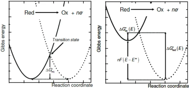
𝑗 = 𝑛𝐹𝑣 = 𝑛𝐹�𝑘𝑜𝑥𝑐𝑅∅− 𝑘𝑟𝑒𝑑𝑐𝑂∅� (1.79) To a first approximation, kinetic constants can be rationalized as the average electron velocity across the interfacial region. According to the transition state theory, the electron transfer rate constants can be expressed in terms of the corresponding potential dependent activation energies Δ𝐺∗_(𝐸): �𝑘𝑜𝑥 = 𝐴𝑒−Δ𝐺 𝑜𝑥∗ (𝐸) 𝑅𝑇 𝑘𝑟𝑒𝑑 = 𝐴𝑒− Δ𝐺_𝑟𝑒𝑑∗ (𝐸) 𝑅𝑇 (1.80)

As shown in Figure 8 (left), the rate constants for oxidation and reduction at the equilibrium potential are equal (𝑘𝑜𝑥 = 𝑘𝑟𝑒𝑑 = 𝑘0). Consequently, the net rate of the

electrochemical reaction is zero. Changes on the potential of the electrode surface 𝐸 with respect to the equilibrium potential 𝐸0_{will shift the equilibrium towards reactants or}

products. Kinetic overpotential 𝜂𝑘𝑖𝑛 is then:

𝜂𝑘𝑖𝑛 = 𝐸 − 𝐸0 (1.81)

Overpotential will affect the activation energies in a different fashion, as showed in Figure 8 (right), and a net current is generated.

(23)

Figure 8. Potential dependent Gibbs free-energy as a function of a reaction coordinate: at the equilibrium (left),

at electrode potentials 𝐸 more positive than the equilibrium potential 𝐸0_(right)

The activation energies are modified by a fraction 𝛼 of the thermodynamic driving force 𝑛𝐹𝜂𝑘𝑖𝑛 (31):

� Δ𝐺𝑜𝑥∗ (𝐸) = Δ𝐺𝑜𝑥∗ (𝐸0) − 𝛼𝑛𝐹𝜂𝑘𝑖𝑛

Δ𝐺𝑟𝑒𝑑∗ (𝐸) = Δ𝐺𝑟𝑒𝑑∗ (𝐸0) + (1 − 𝛼)𝑛𝐹𝜂𝑘𝑖𝑛 (1.82) where 𝛼 is the so-called transfer coefficient (value between 0 and 1). Combining and rearranging equations (1.79), (1.80) and (1.82) we obtain the Butler-Volmer equation (plotted in Figure 9): 𝑗(𝐸) = 𝑗0�𝑒��𝛼𝑛𝐹𝑅𝑇𝜂𝑘𝑖𝑛 j anodic − 𝑒_{��}−(1−𝛼)𝑛𝐹𝑅𝑇𝜂𝑘𝑖𝑛 j cathodic � (1.83)

Where 𝑗0 is known as exchange current density:

𝑗0= 𝑛𝐹𝑘0�𝐶𝑅∅� 1−𝛼

�𝐶𝑂∅�

𝛼 _(1.84)

As any rate constant of a chemical reaction, the exchange current density depends on temperature and reactants/products concentrations as:

𝑗0(𝑇, 𝐶𝑂, 𝐶𝑅) = 𝑗0(𝑇∗, 𝐶𝑂∗, 𝐶𝑅∗) �𝐶_𝐶𝑅 𝑅∗� 𝛾 �𝐶_𝐶𝑂 𝑂∗� 𝛿 𝑒−𝐸𝑅𝑇𝑎𝑐𝑡 (1.85) where 𝛾 and 𝛿 are respectively the reaction order for oxidation and reduction reactions, 𝐸𝑎𝑐𝑡 is the activation energy.

At a narrow potential range around the equilibrium potential (i.e. _|𝜂_𝑘𝑖𝑛_{| ≪ 𝑅𝑇 𝛼𝑛𝐹}⁄ ), the Butler-Volmer equation can be linearized by means of Taylor expansion:

⎩ ⎨ ⎧ 𝑗 ≅𝜂_𝑅𝑘𝑖𝑛 𝑐𝑡 𝑅𝑐𝑡 =_𝑛𝐹𝑗𝑅𝑇 0 (1.86)

(24)

Figure 9. Current - overpotential curves for a kinetically controlled electrochemical reaction Often the Butler-Volmer equation is written in 𝐿𝑜𝑔10 form:

𝑗(𝐸) = 𝑗0�10 𝜂𝑘𝑖𝑛

𝑏𝑟𝑒𝑑 − 10−𝜂 𝑘𝑖𝑛

𝑏𝑜𝑥� (1.87)

where 𝑏𝑟𝑒𝑑 and 𝑏𝑜𝑥 are respectively the reduction and oxidation Tafel slope representing

the overpotential increase required for a ten folds increase in current.

At large overpotentials, the total current is dominated by either the cathodic (reduction) or the anodic (oxidation) process. In this case, the current is expressed as:

�𝐿𝑜𝑔10𝑗 = 𝐿𝑜𝑔10𝑗0+ 𝜂𝑘𝑖𝑛 𝑏𝑎 𝜂𝑘𝑖𝑛 ≥ 𝑏𝑎 𝐿𝑜𝑔10𝑗 = 𝐿𝑜𝑔10𝑗0−𝜂_𝑏𝑘𝑖𝑛 𝑐 𝜂𝑘𝑖𝑛 ≤ 𝑏𝑐 (1.88)

commonly referred to as Tafel equation. Inverting equation (1.88) we obtain the formula for the kinetic overvoltage:

𝜂𝑘𝑖𝑛 = ±𝑏 𝐿𝑜𝑔10_𝑗𝑗

0 (1.89)

Mass-transport losses

Let consider the general electrochemical reaction (1.74) in which the kinetic of electron transfer is infinitely faster than the transport of species from the electrolyte to the electrode surface. For reversible systems, the Nernst equation is established “instantaneously” at the electrode surface:

Δ𝑎𝑞𝑀 𝜙 = Δ𝑀𝑎𝑞𝜙0−𝑅𝑇_{𝑛𝐹 ln �}𝑐𝑅 ∗

𝑐_𝑂∗� (1.90)

where 𝑐0∗ and 𝑐𝑅∗ are the bulk concentration for respectively 𝑂 and 𝑅 species. Changes in

the applied electrode potential 𝐸 modifies the concentration ratio of the redox species at the electrode surface, creating concentration profiles, such that:

𝐸 = Δ𝑀𝑎𝑞𝜙0−𝑅𝑇_{𝑛𝐹 ln �}𝑐𝑅 ∅

(25)

where 𝑐_𝑂∅_{and 𝑐} 𝑅

∅_{are the concentrations at the electrode surface for respectively 𝑂 and}

𝑅 species. Mass-transport overpotential 𝜂𝑡𝑥 is then:

𝜂𝑡𝑥 = 𝑉 − Δ𝑎𝑞𝑀 𝜙 =𝑅𝑇_{𝑛𝐹 ln �}𝑐𝑂 ∅

𝑐𝑂∗� �

𝑐𝑅∗

𝑐_𝑅∅� (1.92)

The region where the concentration of the redox species depends on distance is the diffusion layer or Nernst layer. Local changes in the concentration give rise to an electrical current. The current is proportional to the rate of transformation of O to R, or vice versa. For a reversible process, the current is proportional to the flux 𝐽𝑂 of the reactant to the

electrode surface or to the flux 𝐽𝑅 of the products away from the electrode. Recalling Fick’s

(equation (1.61), the faradic current for the diffusion limited step is simply:

𝑖 = 𝑛𝐹𝐴𝐽𝑂 = −𝑛𝐹𝐴𝐷𝑂�𝜕𝑐_{𝜕𝑥 �}𝑂

𝑥=0= 𝑛𝐹𝐴𝐷𝑅�

𝜕𝑐𝑅

𝜕𝑥 �𝑥=0 (1.93)

where 𝐴 is the geometrical area of the electrode, 𝐷𝑂 and 𝐷𝑅 are the diffusion

coefficients for respectively O and R species, 𝑐𝑂 and 𝑐𝑅 are the molar concentrations for

respectively O and R species, 𝑥 is the distance from the electrode surface. In order to calculate the diffusion limited current, the concentration gradient at the electrode surface (𝑥 = 0) should be established. Let consider the case in which the thickness of the diffusion layer (𝛿) is fixed: 𝑖 = 𝑛𝐹𝐴𝐷0�𝑐𝑂 ∗_{− 𝑐} 𝑂∅ 𝛿𝑂 � = −𝑛𝐹𝐴𝐷𝑅� 𝑐_𝑅∗ _{− 𝑐} 𝑅∅ 𝛿𝑅 � (1.94)

In the limit where the applied potential 𝑉 ≪ Δ𝑀𝑎𝑞𝜙 we can assume an infinitely fast

reduction reaction kinetics, i.e. 𝑐_𝑂∅ _{= 0, reduction current reaches the maximum value 𝑖} 𝑟𝑒𝑑 ∞ _:

𝑖𝑟𝑒𝑑∞ =𝑛𝐹𝐴𝐷0𝑐𝑂 ∗

𝛿𝑂 (1.95)

Similarly when 𝑉 ≫ Δ𝑀𝑎𝑞𝜙, oxidation current reaches the maximum value 𝑖𝑜𝑥∞:

𝑖𝑜𝑥∞ = −𝑛𝐹𝐴𝐷𝑅𝑐𝑅 ∗

𝛿𝑅 (1.96)

Combining equations (1.92), (1.95) and (1.96) we obtain:

𝜂𝑡𝑥 =𝑅𝑇_{𝑛𝐹 ln}��𝑖𝑟𝑒𝑑 ∞ _{− 𝑖}

𝑖 − 𝑖𝑜𝑥∞ � �

𝑖𝑜𝑥∞

𝑖_𝑟𝑒𝑑∞ �� (1.97)

In the case that only one of the redox species is diffusion limited, e.g. 𝑅 is a gas free to leave the electrochemical cell, we obtain:

𝜂𝑡𝑥 =𝑅𝑇_{𝑛𝐹 ln �1 −}_𝑖𝑖 𝑟𝑒𝑑∞ �

(1.98) Ohmic losses

Resistance overpotential 𝜂Ω is due to resistance to electron and ion conduction,

according to the Ohm’s law:

𝜂Ω= 𝑖 𝑅Ω (1.99)

where 𝑅Ω is the sum of all resistances sources (electrode, electrolyte, ion-exchange

membranes and junctions). Electrolyte resistance can be calculated from equation (1.50) or measured by means of Electrochemical impedance spectroscopy (EIS), which allow to measure whole 𝑅Ω, as described in the next section.

(26)

1.2 _{Electrochemical impedance spectroscopy (EIS)}

At an interface, physical properties change precipitously and heterogeneous charge distributions (polarizations) reduce the overall electrical conductivity of a system. The rate at which a polarized region will change when the applied voltage is reversed is characteristic of the type of interface: slow for chemical reactions, appreciably faster across the electrolyte. The emphasis in electrochemistry has consequently shifted from a time/concentration dependency to frequency-related phenomena, a trend toward small-signal alternating current (ac) studies. Electrical double layers and their inherent capacitive reactances are characterized by their relaxation times, or more realistically by the distribution of their relaxation times. The electrical response of a heterogeneous cell can vary substantially depending on the species of charge present, the microstructure of the electrolyte, and the texture and nature of the electrodes.

Electrochemical Impedance Spectroscopy (EIS) or ac impedance methods have seen tremendous increase in popularity in recent years. Initially applied to the determination of the double-layer capacitance (32; 33; 34; 35) and in ac polarography (36; 37), they are now applied to the characterization of electrode processes and complex interfaces. EIS studies the system response to the application of a periodic small amplitude AC signal. These measurements are carried out at different ac frequencies and, thus, the name impedance spectroscopy was later adopted. Analysis of the system response contains information about the interface, its structure and reactions taking place there. EIS is a very sensitive technique and it must be used with great care. Besides, it is not always well understood. This may be connected with the fact that existing reviews on EIS are very often difficult to understand by non-specialists and, frequently, they do not show the complete mathematical developments of equations connecting the impedance with the physico-chemical parameters. It should be stressed that EIS cannot give all the answers. It is a complementary technique and other methods must also be used to elucidate the interfacial processes.

1.2.1 _{Response of Electrical Circuits}

Application of an electrical perturbation (current, potential) to an electrical circuit causes the appearance of a response. In this section, the system response to an arbitrary perturbation and, later, to an ac signal, will be presented.

Arbitrary Input Signal

Let us consider application of an arbitrary (but known) potential 𝐸(𝑡) to a resistance 𝑅. The current 𝑖(𝑡) is given as: 𝑖(𝑡) = 𝐸(𝑡)/𝑅. When the same potential is applied to the series connection of the resistance 𝑅 and capacitance 𝐶, the total potential difference is a sum of potential drops on each element. Taking into account that for a capacitance 𝐸(𝑡) = 𝑄(𝑡) /𝐶, where 𝑄 is the charge stored in a capacitor, the following equation is obtained:

𝐸(𝑡) = 𝑖(𝑡)𝑅 +𝑄(𝑡)_{𝐶 = 𝑖}(𝑡)𝑅 +_𝐶1� 𝑖(𝑡)𝑑𝑡𝑡

0

(27)

This equation may be solved using either Laplace transform or differentiation techniques (38; 39). Differentiation gives: 𝜕𝑖(𝑡) 𝜕𝑡 + 𝑖(𝑡) 𝑅𝐶 = 1 𝑅 𝜕𝐸(𝑡) 𝜕𝑡 (1.101)

which may be solved for known 𝐸(𝑡) using standard methods for differential equations. The Laplace transform is an integral transform in which a function of time 𝑓(𝑡) is transformed into a new function of a parameter 𝑠 called frequency, 𝑓̅(𝑠) or 𝐹(𝑠), according to:

ℒ[𝑓(𝑡)] = 𝑓̅(𝑠) = 𝐹(𝑠) = � 𝑓(𝑡)𝑒∞ −𝑠𝑡_𝑑𝑡

0− (1.102)

The Laplace transform is often used in solution of differential and integral equations. In general, the parameter 𝑠 may be complex, 𝑠 = 𝜈 + 𝑗𝜔, where 𝑗 = √−1. Direct application of the Laplace transform to equation (1.100), taking into account that ℒ �∫ 𝑖(𝑡)𝑑𝑡₀𝑡 �= 𝑖̅(𝑠) 𝑠⁄ ,

gives:

𝐸�(𝑠) = 𝚤̅(𝑠)𝑅 +𝚤̅(𝑠)_𝑠𝐶 (1.103)

which leads to:

𝚤̅(𝑠) = 𝐸�(𝑠)

�𝑅 + 1_𝑠𝐶� (1.104)

The ratio of the Laplace transforms of potential and current, 𝐸�(𝑠)/𝚤̅(𝑠) is expressed in the units of resistance, Ω, and is called impedance, 𝑍̅(𝑠). In this case:

𝑍̅(𝑠) =𝐸�(𝑠)_{𝚤̅(𝑠) = 𝑅 +}_𝑠𝐶1 (1.105)

It should be noticed that the impedance of a series connection of a resistance and capacitance, equation (1.105), is a sum of the contributions of these two elements: resistance, 𝑅, and capacitance, 1/𝑠𝐶. For the series connection of a resistance, 𝑅, and inductance, 𝐿, the total potential difference consists of the potential drop on both elements:

𝐸(𝑡) = 𝑖(𝑡)𝑅 + 𝐿𝜕𝑖(𝑡)_𝜕𝑡 (1.106)

Taking into account that ℒ[𝜕𝑖(𝑡)/𝜕𝑡]= 𝑠 𝑖̅(𝑠)− 𝑖(0+), and taking 𝑖𝑡=0 = 0, one obtains

the current response in the Laplace space:

𝚤̅(𝑠) =_{(𝑅 + 𝑠𝐿)}𝐸�(𝑠) (1.107)

In both cases considered above the system impedance consists of the sum of two terms, corresponding to two elements: resistance and capacitance or inductance. In general, one can write contributions to the total impedance corresponding to the resistance as 𝑅, the capacitance as 1/𝑠𝐶 and the inductance as 𝑠𝐿. Addition of impedances is analogous to the addition of resistances. Knowledge of the system impedance allows for an easy solution of the problem. For example, when a constant voltage, 𝐸0, is applied at time zero to a series

connection of 𝑅 and 𝐶, the current is described by equation (1.104). Taking into account that the Laplace transform of a constant ℒ[𝐸𝑜]= 𝐸0/𝑠, one gets:

(28)

𝚤̅(𝑠) =

𝑠 �𝑅 + 1_𝑠𝐶�= 𝑅 𝑠 + 1_𝑅𝐶 (1.108)

Inverse transform of (1.108) gives the current relaxation versus time:

𝑖(𝑡) =𝐸_{𝑅 𝑒}0 − 𝑡𝑅𝐶 (1.109)

The result obtained shows that after the application of the potential step, current initially equals 𝐸0/𝑅 and it decreases to zero as the capacitance is charged to the potential

difference 𝐸0. Similarly, application of the potential step to a series connection of 𝑅 and 𝐿

produces response given by equation (1.107) which, after substitution of 𝐸�(𝑠) = 𝐸0 /𝑠,

gives:

𝚤̅(𝑠) =_{𝑠(𝑅 + 𝑠𝐿) =}𝐸0 𝐸_{𝑅 �}0 1_{𝑠 +} 1

𝑠 + 𝑅𝐿� (1.110)

Inverse transform gives the time dependence of the current:

𝑖(𝑡) =𝐸_𝑅0�1 − 𝑒−𝑅𝑡𝐿� (1.111)

The current starts at zero as the inductance constitutes infinite resistance at t = 0 and it increases to 𝐸0/𝑅 as the effect of inductance becomes negligible in the steady-state

condition.

In a similar way other problems of transient system response may be solved. In the Laplace space the equations (e.g. equations (1.108) and (1.110)) are much simpler than those in the time space (e.g. equations (1.109) and (1.111)) and analysis in the frequency space s allows for the determination of the system parameters. In the cases involving more time constants, i.e. more than one capacitance or inductance in the circuit, the differential equations describing the system are of the second or higher order and the impedances obtained are the second or higher order functions of 𝑠.

Alternating Voltage (av) Input Signal

In the EIS we are interested in the system response to the application of a sinusoidal signal, i.e. 𝐸(𝑡) = 𝐸0sin (𝜔𝑡), where 𝐸0 is the signal amplitude, 𝜔 = 2𝜋𝑓 is the angular

frequency, and 𝑓 is the av signal frequency. This problem may be solved in different ways. First, let us consider application of an av signal to a series R-C connection. Taking into account that the Laplace transform of the sine function ℒ[sin(ωt)]= 𝜔/(𝑠2_{+ 𝜔}2₎_{, use of} equation (1.104) gives:

𝚤̅(𝑠) =_𝑠₂𝐸_{+ 𝜔}0𝜔 ₂ 1

𝑅 + 1_𝑠𝐶 (1.112)

Distribution into simple fractions leads to:

𝚤̅(𝑠) = 𝐸0 𝑅 �𝜔2_{+ � 1} 𝑅𝐶� 2 � �𝜔2 𝜔 𝑠2_{+ 𝜔}2+ 𝜔 𝑅𝐶 𝑠 𝑠2_{+ 𝜔}2− 𝜔 𝑅𝐶 1 𝑠 + 1_𝑅𝐶� (1.113)

(29)

𝑖(𝑡) = 𝐸0 𝑅 �𝜔2_{+ � 1} 𝑅𝐶� 2 ��𝜔 2_{sin(𝜔𝑡) +} 𝜔 𝑅𝐶 cos(𝜔𝑡) − 𝜔 𝑅𝐶 𝑒− 𝑡𝑅𝐶� (1.114)

The third term in eqn. (15) corresponds to a transitory response observed just after application of the av signal and it decreases quickly to zero. The steady-state equation may be rearranged into a simpler form:

𝑖(𝑡) = 𝐸0

𝑅 �1 + � 1_{𝜔𝑅𝐶�}2�

�sin(𝜔𝑡) +_{𝜔𝑅𝐶 cos(𝜔𝑡)}1 �

(1.115)

and by introducing tan 𝜙 = 1/𝜔𝑅𝐶 the following form is found:

𝑖(𝑡) = 𝐸0

�𝑅2_{+ 1}

(𝜔𝐶)2

sin(𝜔𝑡 + 𝜙) =_{|𝑍| sin}𝐸0 (𝜔𝑡 + 𝜙) _(1.116)

where 𝜙 is the phase-angle between current and potential. It is obvious that the current has the same frequency as the applied potential but is phase-shifted by the angle 𝜙. The value _{|𝑍| has units of resistance; it is the length of a vector obtained by addition of two} perpendicular vectors: 𝑅 and 1/𝜔𝐶.

Complex Notation

In order to simplify the calculations of impedances, the result obtained for the periodic perturbation of an electrical circuit may be represented using complex notation. In the latter example the system impedance, 𝑍(𝑗𝜔), may be represented as:

𝑍(𝑗𝜔) = 𝑍′_{+ 𝑗𝑍′′ = 𝑅 − 𝑗} 1

𝜔𝐶 (1.117)

and the real and imaginary parts of the impedance are: 𝑍′ _{= 𝑅 and 𝑍}′′ _{= −1/𝜔𝐶,}

respectively. It should be noted that the complex impedance 𝑍(𝑗𝜔), equation (1.117), may be obtained from 𝑍(𝑠) equation (1.105), by substitution: 𝑠 = 𝑗𝜔. In fact, this is the imaginary Laplace transform. The modulus of 𝑍(𝑗𝜔), equation (1.116), equals:

|𝑍| = �(𝑍′)2_{+ (𝑍}′′₎2_{= �𝑅}2₊ 1

(𝜔𝐶)2 (1.118)

and the phase-angle between the imaginary and real impedance equals 𝜙 = arg(𝑍) = tan−1_{(−1/𝜔𝑅𝐶). It may be recalled that in complex notation:}

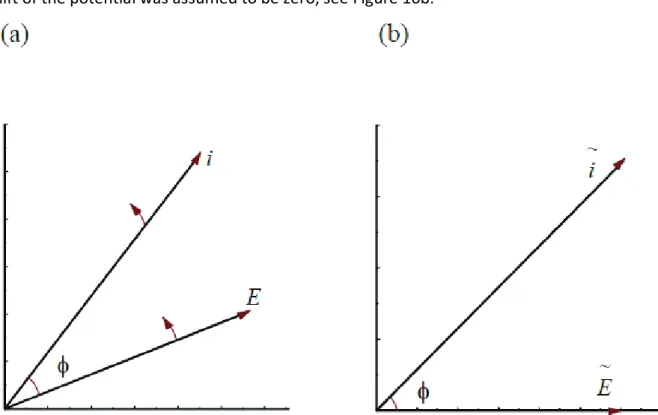
𝑍(𝑗𝜔) = |𝑍|𝑒𝑗𝜙_{= |𝑍|[cos(𝜙) + 𝑗 sin(𝜙)]} _(1.119) Analysis of equation (1.116) indicates that the current represents a vector of the length 𝑖0 = 𝐸0/|𝑍| which rotates with the frequency𝜔. Current and potential are rotating vectors in

the time domain, as represented in Figure 10a. Using complex notation they may be described by:

� 𝐸 = 𝐸0𝑒𝑗𝜔𝑡 𝑖 = 𝑖0𝑒𝑗(𝜔𝑡+𝜙)

(1.120)

These vectors rotate with a constant frequency 𝜔 and the phase-angle, 𝜙, between them stays constant. Instead of showing rotating vectors in time space it is possible to present immobile vectors in the frequency space, separated by the phase-angle 𝜙. These

(30)

vectors are called phasors; they are equal to 𝐸� = 𝐸0 and 𝚤̃ = 𝑖0𝑒

shift of the potential was assumed to be zero, see Figure 10b.

Figure 10. Representation of ac signals: (a) rotating voltage and current vectors in time space; (b) voltage and

current phasors in frequency space

1.2.2 _{Impedance of Electrical Circuits}

Electrical circuit theory distinguishes between linear and non-linear systems (circuits). Impedance analysis of linear circuits is much easier than analysis of non-linear ones. A linear system is one that possesses the important property of superposition: If the input consists of the weighted sum of several signals, then the output is simply the superposition, that is, the weighted sum, of the responses of the system to each of the signals. For a potentiostated electrochemical cell, the input is the potential and the output is the current.

Electrochemical cells are not linear: doubling the voltage will not necessarily double the current. However, Figure 11 shows how electrochemical systems can be pseudo-linear. If you look at a small enough portion of a cell's current versus voltage curve, it appears to be linear. In normal EIS practice, a small (1 to 10 mV) ac signal is applied to the cell. With such a small potential signal the system is pseudo-linear. If the system is non-linear, the current response will contain harmonics of the excitation frequency. Linear systems should not generate harmonics, so the presence or absence of significant harmonic response allows one to determine the systems linearity.

In general, for a sinusoidal signal, i.e. 𝐸(𝑡) = 𝐸0𝑒𝑗𝜔𝑡, the current response is:

𝑖(𝑡) = 𝐸0

�𝑍̂�𝑒𝑗(𝜔𝑡+𝜙) (1.121)

where 𝑍̂ is the complex impedance:

(31)

Figure 11. Current versus Voltage curve showing pseudo-linearity

For a linear systems the complex impedance may be written for any circuit by taking 𝑅 for a resistance, 1/𝑗𝜔𝐶 for a capacitance and 𝑗𝜔𝐿 for an inductance, and applying Ohm’s and Kirchhoff’s laws to the connection of these elements as shown in Table 2.

Component Impedance Resistor _{𝑍̂ = 𝑅} Inductor _{𝑍̂ = 𝑗𝜔𝐿} Capacitor _{𝑍̂ = 1/𝑗𝜔𝐶}

Table 2. Common electrical elements

Notice that the impedance of a resistor is independent of frequency and has no imaginary component. With only a real impedance component, the current through a resistor stays in phase with the voltage across the resistor.

The impedance of an inductor increases as frequency increases. Inductors have only an imaginary impedance component. As a result, the current through an capacitor is phase shifted by -90° with respect to the voltage.

The impedance versus frequency behavior of a capacitor is opposite to that of an inductor. A capacitor's impedance decreases as the frequency is raised. Inductors also have only an imaginary impedance component. The current through an capacitor is phase shifted by 90° with respect to the voltage.

Serial and Parallel Combinations of Circuit Elements

Figure 12. Impedances in series

For linear impedance elements in series (Figure 12) the total impedance is:

𝑍̂ = � 𝑍̂𝑖 𝑖

(32)

Figure 13. Impedances in parallel

For linear impedance elements in parallel (Figure 13) the total impedance is:

1 𝑍̂= � 1 𝑍̂𝑖 𝑖 (1.124) Nyquist and Bode plots

The expression for 𝑍̂ is composed of a real and an imaginary part (equation (1.122)). If the real part 𝑍′ is plotted on the x-axis and the imaginary part 𝑍′′ on the y-axis of a chart, we get a "Nyquist plot". On the Nyquist plot the impedance can be represented as an vector of length _{|𝑍|. The angle between this vector and the x-axis is 𝜙 = arg�𝑍̂�. Each point on the} Nyquist plot is the impedance at one frequency, but you cannot tell what frequency was used to record that point.

If base-10 logarithm of the frequency is plotted on the x-axis and both the absolute values of the impedance and the phase-angle on the y-axis of a chart, we get a “Bode plot”. Unlike the Nyquist plot, the Bode plot does show frequency information.

Figure 14. Parallel R-C circuit

For the parallel R-C connection in Figure 14 the total impedance is:

𝑍̂ = ₁ 1 𝑅 + 𝑗𝜔𝐶 = 𝑅 1 + 𝜔2_𝑅2_𝐶2− 𝑗 𝜔𝑅2_𝐶 1 + 𝜔2_𝑅2_𝐶2 (1.125) or in polar form: 𝑍̂ = �𝑍̂�𝑒𝑗𝜙 _{= �} 𝑅2+ 𝜔2𝑅4𝐶2 (1 + 𝜔2_𝑅2_𝐶2₎2𝑒𝑗 tan −1_{(𝜔𝑅𝐶)} _(1.126)

We notice from equation (1.125) that:

�𝑍′₋𝑅 2� 2 + (𝑍′′₎2 _{= �}𝑅 2� 2 (1.127)

(33)

i.e. the Nyquist plot consists on a semicircle having radius 𝑅/2 and shifted on the x-axis by 𝑅/2, as shown in Figure 15. The frequency at the semicircle maximum equal to: 𝜔 = 1/𝑅𝐶, the circuit’s characteristic breakpoint frequency (inverse of the characteristic time constant). The semicircle is characteristic of a single "time constant".

Figure 15. Nyquist plot for a parallel R-C circuit (R=100Ω,C=20µF) From equation (1.126):

⎩ ⎪ ⎨ ⎪

⎧ 𝜔→0limlog�𝑍̂� = log 𝑅

lim 𝜔→ 1_𝑅𝐶log�𝑍̂� = log 𝑅 2 log�𝑍̂� ≈ − log 𝜔𝐶 𝜔 ≫_𝑅𝐶1 (1.128)

i.e. on the Bode plot impedance modulus would be nearly constant until the frequency is bigger than the characteristic breakpoint frequency, after which would decrease linearly (Figure 16). Moreover when the frequency is equal to the circuit’s characteristic breakpoint frequency, the phase-angle is 45°.

Figure 16. Bode plot for a parallel R-C circuit (R=100Ω,C=20µF)

1.2.3 _{Equivalent circuits elements}

EIS data is commonly analyzed by fitting it to an equivalent electrical circuit model. Most of the circuit elements in the model are common electrical elements such as resistors, capacitors, and inductors. To be useful, the elements in the model should have a basis in the physical electrochemistry of the system.

Synthesis and Physico-Chemical characterization of anion-exchange polymeric materials for electrochemical applications

U

S

P

F

S

M

,

F

N

D

R

S

C

XXIII

SSD

CHIM/05

Synthesis and Physico-Chemical characterization of

anion-exchange polymeric materials for

electrochemical applications

Ph.D. Thesis

S

Antonio Filpi

S

Prof. Francesco Ciardelli

E

E

Prof. Hubert Gasteiger

Summary

Contents

1

Introduction

1.1

Electrochemistry

1.1.1

Thermodynamics

1.1.2

Transport of species in solution

1.1.3

Kinetics

1.2

Electrochemical impedance spectroscopy (EIS)

1.2.1

Response of Electrical Circuits

1.2.2

Impedance of Electrical Circuits

1.2.3

Equivalent circuits elements

_Introduction

_{Electrochemistry}

_{Thermodynamics}

_{Transport of species in solution}

_Kinetics

_{Electrochemical impedance spectroscopy (EIS)}

_{Response of Electrical Circuits}

_{Impedance of Electrical Circuits}

_{Equivalent circuits elements}