Rendiconti per gli Studi
Economici Quantitativi
Editorial Board
Elio Canestrelli (editor) Marco CorazzaPaola Ferretti
This volume has been composed by Paolo Pellizzari
Optimal default boundary in discrete time models . . . 1 Agata Altieri, Tiziano Vargiolu
Mixed-integer non-linear programming methods for mean-variance portfolio selection . . . 21
Mikhail Andramonov, Marco Corazza
An algorithm for the approximation of the asymmetric stable densities using cubic B-splines . . . 35
Luca Barzanti
An analysis of the effects of continuous dividends on the exercise of American options . . . 41
Antonella Basso, Martina Nardon, Paolo Pianca
Jump Process and Brownian Motion in the Portfolio Optimization . . . 69
Federico Bertato, Elio Canestrelli
Budget allocation in the Integrated Communication Mix 89 Alessandra Buratto
Practical Problems in the Numerical Solution of PDE’s in Finance . . . 105
dividends on the exercise of American options
Antonella Basso, Martina Nardon, and Paolo Pianca⋆
Dipartimento di Matematica Applicata Universit`a Ca’ Foscari di Venezia Dorsoduro 3825/E
30123 Venezia - Italy
Abstract. The main aim of this contribution is to analyze the early exercise fea-tures of American-style put options in the presence of a continuously paid dividend yield. In particular, the attention will be focused on the study of the optimal exer-cise policy, which enables to analyze the behavior of the optimal exerexer-cise time and the probability to exercise the option prior to maturity or at the expiration date. Moreover, we will study also the way the early exercise premium of an American option is influenced by the model parameters.
The optimal exercise boundary is instrumental for the early exercise of American-style options. Unfortunately, an analytic formula for this time dependent optimal boundary is not known. To compute an accurate approximation of the optimal ex-ercise boundary we apply a numerical procedure proposed by [Carr, 1998] based on a technique called randomization.
Then a two-step simulation approach is proposed: the numerical approximation of the optimal exercise boundary obtained with Carr’s procedure computed in the first step is embodied in a Monte Carlo simulation method to estimate the desired features of the option. The two-step procedure proposed is applied to a wide sim-ulation analysis in order to investigate the early exercise convenience of American put options and the effects of continuous dividends on the early exercise.
In addition, we analyze how the discrete monitoring bias induced by a Monte Carlo simulation approach affects the early exercise features of American options. Keywords. Option pricing, American options, continuous dividend, optimal exer-cise boundary, Monte Carlo simulation
J.E.L. classification: G13.
M.S.C. classification: 60G40, 60J60, 65C20.
1
Introduction
Most options written on individual equities, and many others on stock indexes and foreign currencies, are American-style options and thus grant the holder of the option the right to exercise the contract at any
⋆Partially supported by M.U.R.S.T., Research program of national interest
time until the option’s expiration date. This is the case, for example, of the options of the official Italian derivatives market IDEM written on individual stocks.
Furthermore, most of all these options are written on assets that pay some dividends, either at discrete times or continuously. On the other hand, the presence of dividends complicates the analysis of the American option features still further.
The main aim of this contribution is to analyze the early exercise features of American-style put options in the presence of a continuously paid dividend yield. The case of options on underlying assets that pay a continuous dividend yield is well known to the literature but it is by far less studied than the discrete dividend case. This second case includes the stock options but in the former we found, for example, the options on indexes or currencies.
In particular, the attention will be focused on the study of the optimal exercise policy, which enables to analyze the behavior of the optimal exercise time and the probability to exercise the option prior to maturity or at the expiration date.
The early exercise premium of an American option represents the premium given to the American option holder over the value of the European option with the same characteristics, for the possibility of early exercising the option. Besides the optimal exercise policy for the holder of an American option, we will study also the way this premium is influenced by the model parameters.
The convenience of the early exercise of an American option de-pends on the comparison between the current price of the underlying security and a critical value. The function which associates to each point in time this critical value is known as optimal or early exercise boundary. The knowledge of the optimal exercise boundary is crucial to the comprehension of the early exercise feature of American-style options. Unfortunately, an analytic formula for this time dependent optimal boundary is not known.
Different numerical approaches have been proposed in the liter-ature to obtain an approximate boundary. In particular, a number of contributions try to define an approximation of the optimal exer-cise boundary in order to calculate the fair value of an American op-tion. Among these, we found [Huang, Subrahmanyam and Yu, 1996], [Omberg, 1987], [Kim, 1990], [Jacka, 1991], [Carr, Jarrow and Myneni, 1992], [Myneni, 1992], [Allegretto et al., 1995], [Broadie and Detemple,
1996], [Carr, 1998], [Ju, 1998], [AitShalia and Lai, 1999] and [Ait Shalia and Lai, 2001], [Little, Pant and Hou, 2000], [Sullivan, 2000], [Bunch and Johnson,2000].
In this contribution, in order to compute an accurate approxima-tion of the optimal exercise boundary we apply a numerical procedure proposed by [Carr, 1998], based on a particular technique called ran-domization, which has proved robust, accurate and computationally efficient and is able to handle the case of a continuous dividend yield. Once computed, the optimal exercise boundary represents a time dependent barrier which allows to define an optimal stopping rule for early exercise of American options. This stopping rule can be used in a Monte Carlo simulation procedure to determine not only the op-tion value but also an estimate of the optimal stopping time and the probability that the option is exercised prior to or at maturity.
Hence, a two-step simulation approach is proposed: the numerical approximation of the optimal exercise boundary obtained with Carr’s procedure, computed in the first step, is embodied in a Monte Carlo simulation method to estimate the desired features of the option.
This two-step procedure is applied to a wide simulation analysis in order to investigate the early exercise convenience of American put options and the effects of continuous dividends on early exercise.
The paper is organized as follows. Section 2 introduces the main properties of the early exercise boundary. Section 3 presents Carr’s randomization approach. In section 4 we discuss and test through a wide empirical research the accuracy of the approximated boundary obtained with Carr’s procedure. In section 5 we study the behavior of the early exercise premium with respect to the values of the model parameters. In section 6 we present a simulation analysis on the effects of continuous dividends on early exercise of American put options. In section 7 we analyze how the discrete monitoring bias induced by a Monte Carlo simulation approach affects the early exercise features of American options. Finally, section 8 presents some conclusions.
2
The early exercise boundary
Let the dynamics of the price St of the underlying asset be governed by the following risk neutralized diffusion process with constant para-meters
where Wt is a standard Wiener process, r > 0 represents the continu-ously compounded risk-free interest rate, δ is the continuous dividend yield payed by the asset and σ is the volatility of the asset returns.
Let us consider an American style put option and let t = 0 be the current time, t = T the option maturity and X the strike price.
It is known that at each time t ∈ [0, T ] there exists a critical price Bt of the underlying asset which separates the exercise region of prices from the continuation region at a given time t ∈ [0, T ]. Indeed, if the current price of the underlying asset is sufficiently low, it will be advantageous to exercise the option immediately, taking advantage of the early exercise feature of American options. The critical price Bt is the asset price below which it is optimal to exercise the American put option; however, Bt can be characterized in different equivalently ways (see [Bunch and Johnson, 2000]).
Hence, the set of critical exercise prices, one for each time 0 ≤ t ≤ T , define a function B of time t, with t ∈ [0, T ], which is called early exercise boundary or optimal exercise boundary
B : [0, T ] → R+. (2)
Formally, the early exercise boundary can be defined as the op-timal solution of a problem of first passage through a boundary; see for example [Carr, 1998] and [Bunch and Johnson, 2000].
Therefore, if the early exercise boundary could be calculated, we would have an optimal stopping rule to decide the exercise strategy for the option. Unfortunately, the function B is not known a priori, but must be determined as part of the solution to the option valuation problem.
The main properties of the optimal exercise boundary B are dis-cussed in [Basso, Nardon and Pianca, 2002b]; for the case r > 0, which is the most interesting from a financial point of view, they can be sum-marized as follows:
1. B is continuously differentiable on the interval [0, T );
2. B is nondecreasing in t (and therefore nonincreasing in time to maturity τ = T − t);
3. BT = X; near expiration we have lim t→T Bt = ( X if δ ≤ r r δX if δ > r; (3)
4. B does not depend on the current price of the underlying asset, S0;
5. B is linearly homogeneous in X.
Moreover, for a finitely-lived American put option the following bounds hold
B∞≤ Bt≤ X, (4)
where B∞
denotes the boundary value of a perpetual American put (which is constant over time; see [Kim, 1990])
B∞= θ θ − 1X, (5) with θ = −(r − δ − σ 2 /2) −p(r − δ − σ2/2)2+ 2σ2r σ2 . (6)
In the non dividend paying case (δ = 0) the expression for B∞
simpli-fies in B∞= [γ/(1 + γ)]X, with γ = 2r/σ2.
A graphical analysis of the behavior of the optimal exercise bound-ary as the model parameters σ, r and δ vbound-ary can be found in [Basso, Nardon and Pianca, 2002b]. The exercise boundary seems to decrease when σ raises, increase with r and diminish with δ.
Some symmetry properties between American call and put options allow to extend the results obtained for the American puts also to American calls; these symmetry results involve not only the price of American calls and puts but also the optimal exercise boundaries of such options. For a comprehensive treatment of the symmetry proper-ties of American options see [Detemple, 2001].
In particular, it is possible to state the following symmetry relation between the current price P0 of an American put option with strike price X written on an asset with current price S0 and the price C0 of an American call option with the same maturity and strike price S0, written on an auxiliary asset with current price X (note the exchange of roles in the two options between S0 and X, on the one hand and r and δ, on the other hand)
Moreover, the corresponding optimal exercise boundaries BP t and BC
t of the American put and call options above defined are connected by the following symmetry relation
BtP(X, r, δ) =
S0X BC
t (S0, δ, r) t ∈ [0, T ].
(8) The linear homogeneity of the boundary with respect to the exer-cise price allows to write the call/put symmetry relation between the boundaries (8) in the following equivalent form which is more com-monly used (see for example [Carr, 1998] and [Carr and Chesney, 1996])
BtP(X, r, δ) = X 2 BC
t (X, δ, r)
. (9)
The call/put symmetry relation between the boundaries (8) or (9) allows to extend the properties 1-5 to the optimal exercise boundary of a call option by making the proper changes; for example, the boundary of a call option is nonincreasing in time.
3
Carr’s randomization approach
As we have seen, an analytic formula for the optimal exercise bound-ary B is not known. However, some numerical approaches have been proposed in the literature that enable to approximate this function; for a review see [Basso, Nardon and Pianca, 2002a].
In this contribution we use a numerical procedure proposed by [Carr, 1998] with the aim of computing an approximation of the price of an American put option. Carr’s approach uses a staircase approx-imation of the boundary and, together with the current option price, provides a good approximation of the initial critical stock price. By looking for the initial critical stock prices at different times to matur-ity it is possible to obtain a good approximation of the boundary on a grid.
Carr’s approach has proved very robust and precise in determin-ing an approximation of the optimal exercise boundary for American put options written on assets which pay no dividends, as shown in [Basso, Nardon and Pianca, 2002a]. Moreover, it can be extended to options which pay a continuous dividend yield. Thus, we have chosen this method to approximate the early exercise boundary also in the case of a dividend paying asset, with the aim of studying the effects of
the payment of a continuously paid dividend yield on the exercise of American put options.
In the rest of this section we briefly recall Carr’s method, which is based on a particular technique called randomization.
According to Carr’s definition, randomization is a procedure for solving a valuation problem which is made up of the following three steps:
1. let the value of one of the model parameters be randomized by assuming a plausible probability distribution for it;
2. compute the expected value of the dependent variable (which is unknown in the fixed parameter model) with respect to the prob-ability distribution assumed for the randomized parameter; 3. let the variance of the distribution governing the parameter
ap-proach zero, holding the mean of the distribution constant at the fixed parameter value.
The randomization approach can be applied to an option valuation problem in different ways, according to the parameter chosen for the randomization and the probability distribution assumed for it. In par-ticular, Carr randomizes the expiration date of the option and assumes for it either an exponential distribution or a gamma distribution with mean equal the fixed maturity T of the option under examination.
More precisely, Carr assumes that the maturity of the randomized American put is determined by a waiting time which depends on the arrivals of a standard Poisson process and is supposed independent of the underlying stock price process and uncorrelated with any market factor.
When the randomized American option is assumed to mature at the first jump of a Poisson process with intensity λ = 1/T , the random maturity ˜T is exponentially distributed with expected value equal to the actual maturity T .
Since the exponential distribution has a memoryless property, the early exercise boundary of this randomized American option turns out to be independent of time; hence the search for the optimal bound-ary can be carried out by taking into account only time stationbound-ary boundaries. More precisely, the fair value of the randomized American put with an exponential distributed maturity is the solution of the following first passage problem through a constant barrier
P0= sup H
IE£e−rtH(X − S
tH)
where tH is the first passage time through the constant barrier H tH = inf{{t ∈ [0, T ] : St ≤ H} ∪ { ˜T }}; (11) here it is assumed that S0 is in the continuation region, so that S0 is greater than the unknown optimal exercise boundary.
When the underlying security does not pay any dividend (δ = 0) the optimal (constant) exercise boundary is given by
H∗= X µ π1RrT π2− Rπ1 ¶η+ε1 , (12) where R = 1/(1 + rT ), η = 1/2 − r/σ2, ε = pη2+ 2/(Rσ2T ), π 1 = (ε − η)/(2ε), π2= (ε − η + 1)/(2ε) (see [Carr, 1998]). The barrier value H∗
provides an approximation for the current value of the critical price, B0.
The assumption of an exponentially distributed maturity leads to simple formulae for the put option price and the current critical price, but these approximations are often too coarse to be used in practice.
To improve the method, [Carr, 1998] proposes to use for the ran-dom option maturity a distribution with a smaller variance, while keep-ing the mean equal to the actual maturity T . To this aim Carr assumes that the randomized option matures at the na-th jump of a standard Poisson process with intensity λ = na/T . Hence the random maturity is gamma distributed with mean T and variance T2/na.
In such a case the exercise boundary of the randomized put takes the form of a staircase and the price of the randomized American put and the initial critical stock price can be determined using a dynamic programming algorithm.
If the underlying security does not pay any dividend, the staircase values of the critical prices of this randomized put can be determined recursively, for m = 1, . . . , na, as follows
Hm= X µ π1RXr∆ c(m)− A(m) ¶η+ε1 (13) where ∆ = T /na, R = 1/(1 + r∆), ε = pη2+ 2/(Rσ2∆) and η, π1 and π2 are defined as before,
c(m)= m−1 X i=0 µm − 1 + i m − 1 ¶ X£πm 2 (1 − π2)i− Rmπ1m(1 − π)i¤, (14)
A(1)= 0 and for m ≥ 2 A(m)= m X j=2 µ X Hm−j+1 ¶η+ε j−1 X k=0 ¡2ε ln¡Hm−j+1 X ¢¢k k! · · j−k−1 X i=0 µj − 1 + i j − 1 ¶ πj1(1 − π1)k+iRjXr∆. (15) As we said in advance, the randomization approach can be ex-tended to American options on dividend paying assets ([Carr, 1998]). When the underlying asset pays a continuous dividend yield, the stair-case values of the critical prices of the randomized American put option are still determined recursively for m = 1, . . . , na but in this case each staircase critical value must be determined numerically by solving an algebraic equation. For m = 1, . . . , na, Hmis implicitly defined by the following equation c(m)− A(m)=µ X Hm ¶η+ε £π1RXr − π2DHmδ¤ ∆, (16) where now η = 1/2 − (r − δ)/σ2, D = 1/(1 + δ∆), c(m)= m−1 X i=0 µm − 1 + i m − 1 ¶ £Dmπm 2 (1 − π2)i− Rmπ1m(1 − π1)i¤ X, (17) A(1)= 0, and for m ≥ 2, A(m)= m X j=2 µ X Hm−j+1 ¶η+ε j−1 X k=0 ¡2ε ln¡Hm−j+1 X ¢¢k k! · · j−k−1 X i=0 µj − 1 + i j − 1 ¶ h πj1(1 − π1)k+iRjXr− − π2j(1 − π2)k+iDjHm−j+1δ i ∆. (18)
By setting δ = 0 in equations (16)-(18) we obtain the explicit solution (13)-(15). The critical value Hm obtained with equation (15) can be used as an initial guess for an iterative solution of equations (16)-(18).
Hnais the critical price at time t = 0 of the randomized put; this
price B0 of a put option with (fixed) maturity T . The critical prices for the other times t > 0 can be obtained with the same procedure, by considering a randomized put with maturity T − t, in turn. Actually, the boundary B can be calculated on a grid which discretizes the time interval [0, T ] by choosing n equally spaced points of amplitude ∆t = T /n and computing the boundary approximations in correspondence with the times 0, ∆t, 2∆t, . . . , T .
4
The accuracy of the randomization boundary
In the previous section we have summarized the randomization ap-proach proposed by Carr. Nevertheless, in the application of the al-gorithm a point becomes important: which is the best choice for the number na of Poisson arrivals?
The variance of the random maturity, T2/n
a, decreases as the num-ber of arrivals na taken into account increases and tends to zero as na tends to infinity. Thus, by increasing the number of arrivals na we expect to improve the accuracy of the solution; however, this entails higher computational costs.
In order to speed up the convergence of the results to the true values, Carr suggests to use the Richardson extrapolation technique.
The N -point Richardson extrapolation of the initial critical price B0, B0R, can be computed as a weighted average of the N approximate initial critical stock prices B(na)
0 = Hna calculated defining na random
arrivals, with na= 1, . . . , N , and can be written as follows BR0 = N X na=1 (−1)N −nanN a na!(N − na)!B (na) 0 . (19)
We have performed some empirical trials in order to study which is the best implementation of Carr’s method: is it the one with or without Richardson extrapolation? And which is the best choice of the number na of Poisson arrivals, on the one hand, and the number N of steps in the Richardson extrapolation, on the other hand?
The trials carried out compare the approximation of the optimal exercise boundary obtained with Carr’s method both with and without Richardson extrapolation for various values of na and N .
In the comparisons carried out, as benchmark which best approx-imates the (unknown) true optimal exercise boundary we have used
Table 1.Average distances between Carr’s approximations of the optimal exercise boundary computed both with and without Richardson extrapolation and the bino-mial boundary as the number naof jumps vary. The results refer to American put
options with T = 1, X = 100, δ = 0, r ∈ { 0.02, 0.06, 0.10 }, σ ∈ { 0.1, 0.2, 0.3, 0.4 }, and are averaged over the 12 options considered; the standard deviations of the distances are reported, too.
naJUMP BOUNDARIES EXTRAPOLATED BOUNDARIES
average standard average standard
na distance deviation distance deviation
1 0.8700 0.4688 – – 2 0.5431 0.2780 0.2321 0.1162 3 0.3970 0.1985 0.0808 0.0457 4 0.3129 0.1548 0.0310 0.0182 5 0.2581 0.1270 0.0193 0.0076 6 0.2193 0.1077 0.0187 0.0073 7 0.1905 0.0935 0.0203 0.0077 8 0.1682 0.0827 0.0215 0.0082 9 0.1504 0.0741 0.0223 0.0085 10 0.1359 0.0671 0.0228 0.0088
the boundary obtained with a binomial method with a high number of time steps. The binomial method used is the improved CRR binomial procedure proposed by [Basso, Nardon and Pianca, 2002a], which ef-fectively reduces the fluctuating behavior of a discrete boundary.
In particular, in the experiments reported we have used a 25 000 time step lattice. More precisely, the time interval [0, T ] has been di-vided into m = 20 000 sub-intervals of length T /m, but we have made the binomial tree start 5 000 steps before time t = 0 (so that the total number of steps in the lattice is n = 25 000) in order to have a wide range of prices already defined since the time at which the option is evaluated.
In order to measure the accuracy of the boundary approximation we have calculated a measure of the distance between the approxim-ated boundary and the boundary obtained with the binomial method. The distance between these functions has been computed as the norm of the difference between the pair of functions compared, using the discrete norm in L1 (see e.g. [Gautschi, 1997])
dist (Bbin, BCarr) = n−1 X i=0 ¯ ¯ ¯B bin i − BiCarr ¯ ¯ ¯ , (20)
Table 2. Average distances between Carr’s approximations of the optimal exer-cise boundary computed both with and without Richardson extrapolation and the binomial boundary as the number naof jumps and the number N of extrapolated
points vary. The results refer to American put options with T = 1, X = 100, δ ∈ {0.00, 0.02, 0.06, 0.10}, r ∈ { 0.02, 0.06, 0.10 }, σ ∈ { 0.1, 0.2, 0.3, 0.4 }. Columns 2 and 3 show the average and the standard deviation obtained for the 12 cases with zero dividends, columns 4 and 5 indicate the average and the standard devi-ation obtained for the 36 cases with positive dividends and the last two columns report the overall mean and standard deviation computed over all the 48 options considered.
δ = 0 δ > 0 OVERALL MEAN
average standard average standard average standard
distance deviation distance deviation distance deviation
na naJUMP BOUNDARIES 1 0.8700 0.4688 0.8881 0.8578 0.8836 0.7743 2 0.5431 0.2780 0.5649 0.5479 0.5594 0.4917 3 0.3970 0.1985 1.1571 1.0634 0.9630 0.9785 N EXTRAP. BOUNDARIES 2 0.2321 0.1162 0.2506 0.2423 0.2460 0.2166 3 0.0808 0.0457 5.0888 4.2960 3.8101 4.3028
where Bbinand BCarrdenote the boundary obtained with the binomial and Carr’s methods, respectively. In the tables which summarize the results we have reported the distance divided by the number n of points in time
1
n dist (Bbin, BCarr) = 1nPn−1i=0 ¯ ¯Bbin
i − BiCarr ¯
¯, (21)
which corresponds to use a weighted norm with constant weights equal to 1/n. This quantity is the average point error and is easy to inter-pret; moreover, it allows a comparison between trials which rely on a different number of time intervals.
In the trials carried out the early exercise boundaries have been computed in a grid of n + 1 equally spaced points in the interval [0, T ], with n = 250 and T = 1.
Tables 1 and 2 compare the average distances between Carr’s ap-proximations of the optimal exercise boundary computed both with and without Richardson extrapolation and the binomial boundary as the number naof jumps and the number N of extrapolated points vary. The results refer to American put options with T = 1, X = 100, δ ∈ {0.00, 0.02, 0.06, 0.10}, r ∈ { 0.02, 0.06, 0.10 }, σ ∈ { 0.1, 0.2, 0.3, 0.4 }.
Table 1 reports the average distances and the standard deviations of these distances computed over the options written on non dividend paying assets while table 2 reports the same results computed over all the 48 options considered.
An analysis of the results of tables 1 and 2 indicates that, while the accuracy of the boundary approximation is very stable for the non di-vidend paying case, even when the number of jumps is high, when the underlying asset pays a positive dividend yield the boundary approx-imation becomes unstable as soon as the number of jumps is greater than two; for a number of jumps greater than three the numerical procedures of the algorithms rarely gets a result.
As a consequence, for the non dividend paying case we may well use a high number of jumps in order to reduce the approximation error. In this case we may see from table 1 that the use of the Richardson extrapolation procedure effectively reduces this error. However, it is not convenient to apply the Richardson extrapolation with a number of points greater than 6, as the approximation error tends to increase above this value. In particular, when extrapolating on the basis of too points the results tend to be less stable. The best choices turn out to be 5 or 6 extrapolation points, so in the rest of the empirical research we have applied Carr’s approach in conjunction with an extrapolation procedure with N = 5 extrapolated points.
On the other hand, the best choice for the case with a positive dividend yield turns out to be Carr’s approach with a 2-points extra-polation procedure, and this is our choice for this case in the rest of the empirical analysis. Of course, the low number of jumps and extra-polated points used in the computations entails that in the dividend paying case we will get higher approximation errors.
[Basso, Nardon and Pianca, 2002a] presents a detailed analysis of the performance of Carr’s approximation of the optimal exercise bound-ary in the absence of dividends. However, the results of tables 1 and 2 indicate that the performance of the method changes in the presence of dividends; in particular, we expect the approximation of the bound-ary to be less accurate. In order to test the goodness of the boundbound-ary approximation in the presence of a positive dividend yield we have carried out a wide empirical analysis.
We have randomly generated 7 200 option valuation problems with a Monte Carlo procedure. More precisely, we have let the parameters (δ, r, σ) vary in the set [0.005, 0.12] × [0.005, 0.12] × [0.1, 0.4], have
par-Table 3.Average distance and standard deviation of the distance between Carr’s approximation of the boundary and the binomial boundary, as the maturity T varies. The results refer to American put options with X = 100 and are computed over all the 7 200 option valuation problems randomly generated for each maturity in columns 2-3, while they are separated into the zero dividend case and the positive dividend yield case in columns 4-5 and 6-7.
δ ∈ [0.0, 0.12] δ = 0 δ > 0
T average st.dev. of average st.dev. of average st.dev. of
distance distance distance distance distance distance
1/12 0.1905 0.3041 0.0223 0.0120 0.2314 0.3349
1/4 0.1850 0.2920 0.0193 0.0073 0.2214 0.3201
1/2 0.1844 0.2640 0.0185 0.0054 0.2222 0.2854
3/4 0.1844 0.2385 0.0186 0.0050 0.2252 0.2539
1 0.1855 0.2179 0.0189 0.0052 0.2272 0.2278
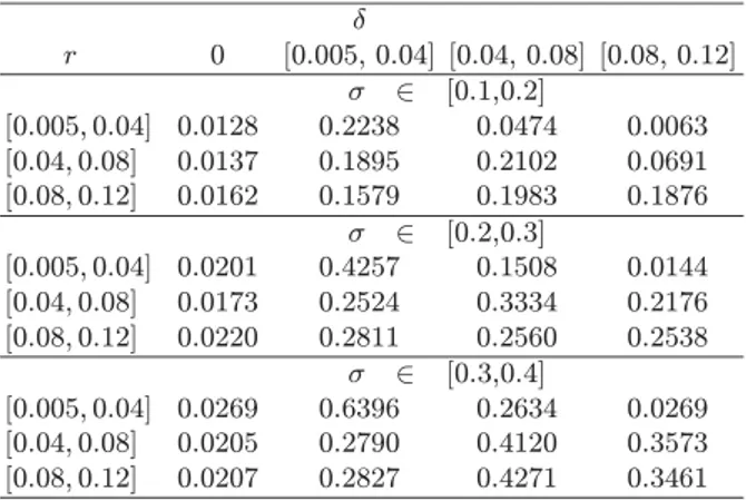
Table 4.Average distance between Carr’s approximation of the boundary and the binomial boundary, as δ, r and σ vary in the intervals indicated, for American put options with maturity T = 1 and X = 100. The results refer to 200 randomly generated problems in each subinterval.
δ r 0 [0.005, 0.04] [0.04, 0.08] [0.08, 0.12] σ ∈ [0.1,0.2] [0.005, 0.04] 0.0128 0.2238 0.0474 0.0063 [0.04, 0.08] 0.0137 0.1895 0.2102 0.0691 [0.08, 0.12] 0.0162 0.1579 0.1983 0.1876 σ ∈ [0.2,0.3] [0.005, 0.04] 0.0201 0.4257 0.1508 0.0144 [0.04, 0.08] 0.0173 0.2524 0.3334 0.2176 [0.08, 0.12] 0.0220 0.2811 0.2560 0.2538 σ ∈ [0.3,0.4] [0.005, 0.04] 0.0269 0.6396 0.2634 0.0269 [0.04, 0.08] 0.0205 0.2790 0.4120 0.3573 [0.08, 0.12] 0.0207 0.2827 0.4271 0.3461
titioned the parameter space with a 3 × 3 × 3 grid into 27 rectangular subsets and have randomly generated 200 (δ, r, σ) triples from each subset, for a total of 5 400 option valuation problems with a positive dividend yield. In addition, we have randomly generated 1 800 option valuation problems with zero dividend by setting δ = 0 and letting the
parameters (r, σ) vary in the set [0.005, 0.12] × [0.1, 0.4] with the same generation rule.
For each generated problem, 5 different maturities have been con-sidered: 1, 3, 6, 9, 12 months. The optimal exercise boundaries have been computed in a grid of n + 1, with n = 250, equally spaced points in the interval [0, 1], so that the monitoring interval is approximately one working day.
Tables 3 and 4 summarize the main results of these trials. In par-ticular, Table 3 reports, for the 5 maturities analyzed, the average dis-tance (21) between the binomial boundary used as benchmark and the approximated boundary obtained with Carr’s method and the stand-ard deviation of this distance. We may observe that the accuracy of Carr’s approximation of the boundary does not vary with time to maturity. Moreover, as it can be seen, in the presence of a positive dividend yield the distance between the approximated and the bench-mark boundary is on average 10 times the distance we observe with zero dividend. On the whole, the boundary approximation may be considered as sufficient for practical purposes, since it entails an ap-proximation error of about 2 % of the exercise price.
Table 4 reports the average distance obtained for T = 1 year separ-ately for the different parameter intervals. It can be observed that the approximation error increases with the volatility σ while a clear pat-tern does not seem to emerge with respect to the values of the interest rate r and the dividend yield δ > 0.
5
The behavior of the early exercise premium
Let us denote by Pt and pt the values at time t of an American and a European put option with analogous characteristics. Then the early exercise premium of the American put option
et= Pt− pt≥ 0 (22)
represents the advantage that the American option has over the Euro-pean contract and measures the advantage of being able to exercise the option at any time until maturity.
The early exercise premium can be written using different rep-resentations (see for example [Elliott and Kopp, 1999], [Kwok, 1998] and [Myneni, 1992]); [Kim, 1990], [Jacka, 1991] and [Carr, Jarrow and
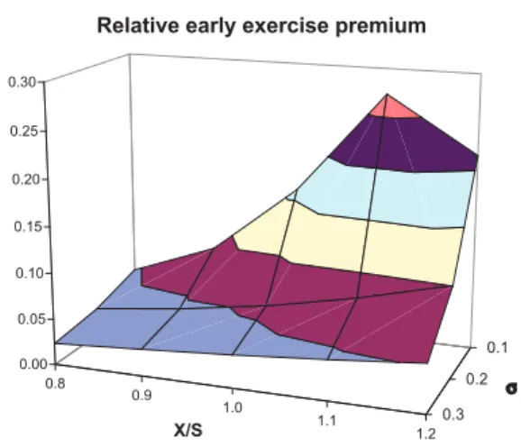
0.8 0.9 1.0 1.1 1.2 0.1 0.2 0.3 0.00 0.05 0.10 0.15 0.20 0.25 0.30 X/S σ Relative early exercise premium
Fig. 1. Relative early exercise premium of American put options as σ and X/S vary. Each result is the average computed over δ and r, with δ ∈ {0.00, 0.02, 0.04, 0.06, 0.08, 0.10} and r ∈ {0.02, 0.04, 0.06, 0.08, 0.10}, while S0 =
100 and T = 1.
Myneni, 1992] provide the following integral representation et= rX Z T t e−r(u−t)N (−d2(St, Bu, u − t)) du − − δSt Z T t e−δ(u−t)N (−d1(St, Bu, u − t)) du (23) where N (·) is the cumulative distribution function of the standard normal random variable,
d1(St, Bu, u − t) = log St/Bu+ (r − δ + σ 2 /2)(u − t) σ√u − t (24) and d2(St, Bu, u − t) = d1− σ √ u − t. (25)
Equation (23), as the other representations proposed in the lit-erature, does not enable to calculate the early exercise premium of American options in closed form. We have used a binomial method
0.00 0.02 0.04 0.06 0.08 0.10 0.02 0.04 0.06 0.08 0.10 0.00 0.05 0.10 0.15 0.20 0.25 0.30 0.35 0.40 0.45 0.50 δ r
Relative early exercise premium
Fig. 2. Relative early exercise premium of American put options as δ and r vary. Each result is the average computed over σ and X/S, with X/S ∈ {0.8, 0.9, 1.0, 1.1, 1.2} and σ ∈ {0.1, 0.2, 0.3}, while S0= 100 and T = 1.
with 25 000 steps in order to analyze the behavior of the early exercise premium of a put option with respect to the various model parameters. To this aim we have carried out a set of trials by evaluating 450 American put options with maturity T = 1 written over assets with S0 = 100, δ ∈ {0.00, 0.02, 0.04, 0.06, 0.08, 0.10}, r ∈ {0.02, 0.04, 0.06, 0.08, 0.10}, moneyness X/S ∈ {0.8, 0.9, 1.0, 1.1, 1.2} and σ ∈ {0.1, 0.2, 0.3}.
Figures 1 and 2 show the behavior of the relative early exercise premium, defined as the ratio between the early exercise premium and the value of the European option with analogous features
erel = e0 p0
= P0− p0 p0
. (26)
The relative early exercise premium increases with the interest rate r and with the moneyness ratio X/S and decreases as the volatility σ increases, while it does not always exhibit a monotone behavior with respect to the value of the dividend yield δ.
For a recent econometric study of the early exercise of American put in the Swedish equity option market see [Engstrom and Norden, 2000].
6
A simulation analysis of the effects of continuous
dividends on early exercise
The financial literature has often taken up the subject of the effects of the payment of one or more discrete dividends on the early ex-ercise of American-style options. On this subject see, for example, [Geske and Shastri, 1985], [Omberg, 1987] and [Meyer, 2002], who study the cases of cash payments of either a known size (independent on the value of the asset) or a known dividend rate (in which the amount of the dividend is proportional to the asset price); for an empirical test of the rationality of the early exercise decision of American options written on equities of the Sweden market both with and without a cash dividend see also [Overdahl and Martin, 1994].
American options written on indexes or foreign currencies, however, rather fall within the category of options written on an underlying asset which pays a continuous dividend yield. Therefore, it is interesting also the investigation of the effects of the payment of a positive dividend yield on the early exercise of American options.
To this aim, we have carried out a wide empirical analysis by means of a two-step procedure. In the first step we have computed an approx-imation of the optimal exercise boundary using the Carr’s randomiz-ation approach presented in the previous sections. In the second step we have embodied the optimal exercise boundary thus obtained in a Monte Carlo simulation procedure.
Actually, the optimal exercise boundary can be regarded as a time dependent barrier which enables to define a stopping rule in order to check the convenience of early exercise of American options. This stopping rule can be embodied in a Monte Carlo simulation method by exploiting the fact that the forward procedure of a simulation method allows to determine an estimate of the first passage times tB in the various simulated paths (see [Basso, Nardon and Pianca, 2002b]). This method enables to determine, besides the option value, also the optimal exercise time, the probability that the option is exercised and the probability of early exercise.
The main advantage of this approach is that the knowledge of the optimal exercise boundary allows to implement a simple forward Monte Carlo procedure which avoids the complications inherent in other sim-ulation approaches proposed for the valuation of American options; for a review of such approaches see [Boyle, Broadie and Glasserman, 2001].
Table 5.Simulation based estimates of the optimal exercise time of American put options with T = 1 as σ, X/S, r, and δ vary. Each result is the average computed over r and δ in the first part of the table and over σ and X/S in the second part; 100 000 paths have been simulated for each option. ˆt∗(·) denotes the mean exercise
time averaged over all the parameters but the one within parentheses. Average optimal exercise times computed over δ and r
X/S σ 0.8 0.9 1.0 1.1 1.2 ˆt∗(σ) 0.1 0.9586 0.9032 0.7479 0.4505 0.3308 0.6782 0.2 0.9286 0.8786 0.7987 0.6746 0.5018 0.7565 0.3 0.9085 0.8678 0.8129 0.7424 0.6536 0.7970 ˆ t∗(X/S) 0.9319 0.8832 0.7865 0.6225 0.4954
Average optimal exercise times computed over X/S and σ δ r 0.00 0.02 0.04 0.06 0.08 0.10 tˆ∗(r) 0.02 0.6882 0.8223 0.9975 1.0000 1.0000 1.0000 0.9180 0.04 0.6074 0.6705 0.7729 0.9720 0.9971 0.9996 0.8366 0.06 0.5548 0.5928 0.6554 0.7482 0.9340 0.9858 0.7452 0.08 0.5093 0.5399 0.5838 0.6431 0.7274 0.8927 0.6493 0.10 0.4759 0.4979 0.5333 0.5753 0.6309 0.7096 0.5705 ˆ t∗(δ) 0.5671 0.6247 0.7086 0.7877 0.8579 0.9175
The simulation analysis regards 450 different options with maturity T = 1 and the following parameter setting: δ ∈ { 0, 0.02, 0.04, 0.06, 0.08, 0.1 }, r ∈ { 0.02, 0.04, 0.06, 0.08, 0.1 }, σ ∈ { 0.1, 0.2, 0.3 }, X/S ∈ { 0.8, 0.9, 1, 1.1, 1.2 }. The simulation estimates are based on the generation of 100 000 simulated paths with n = 250 (daily) time steps.
In the Monte Carlo simulation procedure the optimal exercise time t∗
is estimated by the average passage time through the boundary B of the simulated trajectories, computed over the paths which lead to the option exercise
ˆ t∗= 1 |E| X k∈E tkB, (27)
Table 6. Relative exercise frequencies in the simulation trials carried out as σ, X/S, r, and δ vary. Each result is the average computed over σ and X/S; 100 000 paths have been simulated for each option. ˆp(·) and ˆpa(·) denote the relative exercise
frequencies and the relative early exercise frequencies, respectively, averaged over all the parameters but the one within parentheses.
Average relative exercise frequencies δ r 0.00 0.02 0.04 0.06 0.08 0.10 p(r)ˆ 0.02 0.5089 0.5220 0.5520 0.5827 0.6130 0.6433 0.5703 0.04 0.5057 0.5129 0.5251 0.5516 0.5826 0.6134 0.5485 0.06 0.4990 0.5098 0.5159 0.5272 0.5516 0.5832 0.5311 0.08 0.4955 0.5038 0.5119 0.5201 0.5292 0.5520 0.5188 0.10 0.4904 0.5001 0.5069 0.5146 0.5248 0.5320 0.5115 ˆ p(δ) 0.4999 0.5097 0.5223 0.5392 0.5602 0.5848
Average relative early exercise frequencies δ r 0.00 0.02 0.04 0.06 0.08 0.10 ˆpa(r) 0.02 0.4732 0.4496 0.0114 0.0003 0.0000 0.0000 0.1557 0.04 0.4799 0.4831 0.4610 0.0847 0.0133 0.0024 0.2541 0.06 0.4793 0.4872 0.4920 0.4677 0.1736 0.0488 0.3581 0.08 0.4801 0.4861 0.4922 0.5004 0.4735 0.2507 0.4472 0.10 0.4780 0.4860 0.4911 0.4971 0.5084 0.4791 0.4899 ˆ pa(δ) 0.4781 0.4784 0.3895 0.3101 0.2337 0.1562
where E denotes the set of simulated paths in which the option has been exercised and tk
B is the first passage time through B for the k-th trajectory.
In the empirical analysis the probability to exercise the option is estimated by the relative frequency of exercise ˆp = |E|/N, where N denotes the number of simulated paths. Analogously, the probability to exercise before maturity is estimated by the relative frequency of early exercise ˆpa = |A|/N, where A is the set of the trajectories in which the option has been exercised before maturity (A = { k : tk
B < T }). The simulation results are presented in tables 5-6. Moreover, figures 3-5 show the behavior of the put option price, the optimal exercise time
0.00 0.02 0.04 0.06 0.08 0.10 0.02 0.04 0.06 0.08 0.10 7 8 9 10 11 12 13 14 δ r
Monte Carlo price
Fig. 3.Simulation based estimates of the price of American put options with T = 1 as δ and r vary; S0 = 100. Each result is the average computed over X/S ∈
{0.8, 0.9, 1.0, 1.1, 1.2} and σ ∈ {0.1, 0.2, 0.3}; 100 000 paths have been simulated for each option.
and the relative frequency of early exercise with respect to the values of the dividend yield δ and the interest rate r.
Table 5 summarizes the results concerning the optimal exercise times. In order to investigate the behavior of the exercise time as the parameter values vary table 5 reports the outcomes for different aggreg-ation levels. The first part of the table exhibits the marginal averages of the mean exercise time ˆt∗
computed with respect to the values of δ and r, as the value of X/S and σ vary; for example the first element in the matrix (0.9586) is the mean value of ˆt∗
obtained when σ = 0.1, X/S = 0.8 and the resulting exercise times are averaged over all the values of r and δ. The second part of table 5 reports the marginal averages of ˆt∗
computed with respect to X/S and σ, as the value of δ and r vary. In addition, the table shows the marginal averages of ˆt∗ computed over all the parameters but one (for example ˆt∗
(X/S) is the marginal average computed with respect to σ, r and δ).
As can be seen from table 5, the average optimal exercise time decreases when the moneyness increases. On the contrary, this time is decreasing with respect to the volatility for the lowest moneyness
0.00 0.02 0.04 0.06 0.08 0.10 0.02 0.04 0.06 0.08 0.10 0.40 0.50 0.60 0.70 0.80 0.90 1.00 δ r
Average exercise time
Fig. 4. Simulation based estimates of the optimal exercise time of American put options with T = 1 as δ and r vary. Each result is the average computed over X/S ∈ {0.8, 0.9, 1.0, 1.1, 1.2} and σ ∈ {0.1, 0.2, 0.3}; 100 000 paths have been simulated for each option.
ratios but it is increasing with the volatility for the highest values of the moneyness. Moreover, the optimal exercise time is decreasing with respect to the risk-free interest rate r and increasing with the dividend yield δ.
Table 6 presents the outcomes regarding the relative frequencies of exercise ˆp (first part of the table) and those of early exercise ˆpa (second part of the table), averaged over X/S and σ, as the value of δ and r vary; of course, the difference ˆp − ˆpa gives the relative frequency of exercise at maturity. ˆp(·) and ˆpa(·) denote the marginal averages of ˆ
p and ˆpa, respectively, computed over all the parameters but one. From table 6 we may observe that while the overall exercise fre-quency ˆp increases with the value of the dividend yield δ and decreases as the interest rate r increases, the early exercise frequency ˆpabehaves differently. Actually, the early exercise frequency exhibits a particular behavior with respect to δ and r: it is on average about 50 % for all the cases with δ ≤ r while it is markedly lower for the cases with δ > r (just the cases in which the overall exercise frequency is higher). This behavior is well depicted in figure 4.
0.00 0.02 0.04 0.06 0.08 0.10 0.02 0.04 0.06 0.08 0.10 0.00 0.20 0.40 0.60 0.80 1.00 δ r
Early exercise frequency
Fig. 5. Average relative early exercise frequency of American put options with T = 1 in the simulation trials carried out as δ and r vary. Each result is the average computed over X/S ∈ {0.8, 0.9, 1.0, 1.1, 1.2} and σ ∈ {0.1, 0.2, 0.3}; 100 000 paths have been simulated for each option.
The reasons of this feature are related to the behavior of the bound-ary B near expiration (see limit (3)): when δ > r, B is not continuous at maturity since its left limit is lower that the strike price X. This means that when the ratio r/δ decreases, the probability of early ex-ercise diminishes while at the same time the probability of exex-ercise at maturity increases.
7
Discrete monitoring bias of the simulation method
We have seen in the previous section that the forward procedure of a simulation method allows to determine an estimate of the first pas-sage times tB in the various simulated paths. However, the estimate of the first passage times obtained in such a way will be affected by a bias due to discrete monitoring. This bias is connected to the fact that we can only monitor the prices at discrete points in time: by proceeding in discrete time we neglect what happens between two ad-jacent points; in particular, we do not test continuously if the op-timal stopping boundary is touched. Of course, this bias vanishes
when the monitoring interval ∆t tends to 0. For a discussion of the problem of discrete monitoring bias in path-dependent derivatives see [Broadie, Glasserman and Kuo, 1997], [Broadie, Glasserman and Kuo, 1999] and [Basso and Pianca, 2000]).
We have carried out a set of simulation trials with the aim of study-ing the effects of the discrete monitorstudy-ing bias which affects the two-step simulation method proposed on the early exercise features (exercise time and probability to exercise before maturity) of an American put option. In addition, we have analyzed also the effects of the bias on the price and the probability of exercise of an American put option. Table 7 presents the main results by highlighting the influence of the value of the dividend yield.
Table 7 reports, as the monitoring step varies, the behavior of the simulation estimate ˆP of the option price, its relative error with re-spect to the American option price computed with the CRR binomial method with 25 000 steps, the simulation estimates of the optimal ex-ercise time ˆt∗
, the average early exercise time ˆta, defined by restricting the computation of the first passage time average to the paths in the set A of the trajectories in which the option has been exercised before maturity ˆ ta = 1 |A| X k∈A tkB, (28)
the relative exercise frequency ˆp, the relative early exercise frequency ˆ
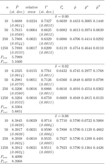
pa and the relative frequency of exercise at maturity ˆpT = ˆp − ˆpa. The discrete monitoring steps taken into consideration correspond roughly to monthly, weekly, daily and infra-daily (5 points a day) frequencies. As it can be observed, when the number of monitoring steps in-creases the relative error of the option price dein-creases but much more relevant are the effects on the exercise time and the exercise probabil-ities. The estimation of the optimal exercise time diminishes heavily as the number of steps increases while at the same time the average early exercise time slightly rises. On the other hand, still most remarkable are the effects on the exercise probabilities: whereas the overall relat-ive exercise frequency barely rises, we may note that the early exercise frequency undergoes a considerable increase while at the same time the frequency of exercise at maturity drops.
Table 7.Simulation results for American put options as the number n of monitor-ing steps vary, for different values of δ, X = S0= 100, r = 0.06, σ = 0.2 and T = 1.
100 000 paths have been simulated for each problem. The values in italics within parenthesis denote the standard deviation. Pamis the American option price
com-puted with a binomial method with 25 000 steps, Peur the price of the analogous
European option.
n Pˆ relative ˆt∗ tˆ∗
a pˆ pˆa pˆT
(st. dev.) error (st. dev.)
δ = 0.00 10 5.6688 0.0224 0.7327 0.6039 0.4453 0.3005 0.1448 (0.0614 ) (0.0012 ) 50 5.7615 0.0064 0.6625 0.6082 0.4613 0.3974 0.0639 (0.0568 ) (0.0012 ) 250 5.7868 0.0021 0.6329 0.6086 0.4706 0.4414 0.0292 (0.0544 ) (0.0012 ) 1250 5.7893 0.0017 0.6209 0.6119 0.4754 0.4644 0.0110 (0.0533 ) (0.0012 ) Pam 5.7989 Peur 5.1660 δ = 0.02 10 6.2325 0.0155 0.7761 0.6432 0.4745 0.2977 0.1768 (0.0614 ) (0.0011 ) 50 6.2981 0.0051 0.7126 0.6560 0.4848 0.4050 0.0798 (0.0579 ) (0.0011 ) 250 6.3206 0.0016 0.6866 0.6616 0.4916 0.4554 0.0362 (0.0560 ) (0.0011 ) 1250 6.3204 0.0016 0.6759 0.6669 0.4948 0.4815 0.0133 (0.0552 ) (0.0011 ) Pam 6.3304 Peur 5.8851 δ = 0.08 10 8.3845 0.0029 0.9714 0.7710 0.5790 0.0722 0.5068 (0.0628 ) (0.0004 ) 50 8.3917 0.0021 0.9590 0.7898 0.5790 0.1129 0.4662 (0.0626 ) (0.0004 ) 250 8.3938 0.0018 0.9535 0.7927 0.5790 0.1299 0.4491 (0.0624 ) (0.0005 ) 1250 8.3912 0.0021 0.9511 0.7923 0.5790 0.1364 0.4426 (0.0624 ) (0.0005 ) Pam 8.4090 Peur 8.3968
8
Conclusions
In this paper we have studied the exercise features of American put options written on assets which pay a continuous dividend yield and analyzed the effects of dividends on the early exercise. To this aim we have used a two-step procedure.
In the first step we have obtained an approximation of the op-timal exercise boundary using the randomization approach proposed by [Carr, 1998]. The accuracy of this approximated boundary is tested through a wide computational experience. In the second step we have embodied the optimal exercise boundary thus computed in a Monte Carlo simulation procedure.
Then we have studied early exercise and the effects of dividends by carrying out a wide simulation analysis.
Finally, we have analyzed the effects on the option price and the early exercise estimation (mainly on the exercise time and the probab-ility of exercise) of the bias due to the discrete monitoring procedure implemented in a Monte Carlo simulation approach.
Further investigation, left for future research, concerns the possib-ility to apply proper corrections to the simulation procedure in order to reduce or eliminate the discrete monitoring bias.
References
[AitShalia and Lai, 1999] AitShalia F. and Lai T.L. (1999). A Canonical Optimal Stopping Problem for American Options and its Numerical Solution. Journal of Computational Finance, 3:33–52.
[AitShalia and Lai, 2001] AitShalia F. and Lai T.L. (2001). Exercise Boundaries and Efficient Approximations to American Option Prices and Hedge Parameters. Journal of Computational Finance, 4:85–103.
[Allegretto et al., 1995] Allegretto W., Barone-Adesi G. and Elliott R.J. (1995). Numerical Evaluation of the Critical Price and American Options. The European Journal of Finance, 1:69–78.
[Basso, Nardon and Pianca, 2002a] Basso A., Nardon M. and Pianca P. (2002). Discrete and Continuous Time Approximations of the Optimal Exercise boundary of American options. Quaderni del Dipartimento di Matematica Applicata, n. 105/2002, Universit`a “Ca’ Foscari” di Venezia.
[Basso, Nardon and Pianca, 2002b] Basso A., Nardon M. and Pianca P. (2002). Optimal Exercise of American Options. Quaderni del Dipartimento di Matematica Applicata, n. 106/2002, Universit`a “Ca’ Foscari” di Venezia.
[Basso and Pianca, 2000] Basso A. and Pianca P. (2000). Correcting Simulation Bias in Discrete Monitoring of Russian Options. Quaderni del Dipartimento di Matematica Applicata alle Scienze Economiche Statistiche e Attuariali “Bruno De Finetti”, n. 8/2000, Universit`a degli Studi di Trieste.
[Boyle, Broadie and Glasserman, 2001] Boyle P.P., Broadie M. and Glasserman P. (2001). Monte Carlo methods for security pricing. In Jouini E., Cvitanic J. and Musiela M. (eds.) (2001). Option Pricing, Interest Rates and Risk Management. Cambridge University Press, Cambridge, 185–238.
[Broadie and Detemple, 1996] Broadie M. and Detemple J. (1996). American Op-tion ValuaOp-tion: New Bounds, ApproximaOp-tions, and a Comparison of Existing Methods. Review of Financial Studies, 9:1211–1250.
[Broadie, Glasserman and Kuo, 1997] Broadie M., Glasserman P. and Kuo S. (1997). A continuity correction for discrete barrier options. Mathematical Fin-ance, 7:325–349.
[Broadie, Glasserman and Kuo, 1999] Broadie M., Glasserman P. and Kuo S. (1999). Connecting discrete and continuous path-dependent options. Finance and Stochastics, 3:55–82.
[Bunch and Johnson, 2000] Bunch D.S. and Johnson H. (2000). The American Put Option and Its Critical Stock Price. Journal of Finance, 55:2333–2356.
[Carr, 1998] Carr P. (1998). Randomization and the American Put. Review of Financial Studies, 11:597–626.
[Carr and Chesney, 1996] Carr P. and Chesney M. (1998). American Put Call Symmetry. Working Paper.
[Carr, Jarrow and Myneni, 1992] Carr P., Jarrow R. and Myneni R. (1992). Al-ternative Characterizations of American Put. Mathematical Finance, 2:229–263. [Detemple, 2001] Detemple J. (2001) American Options: Symmetry Properties. In Jouini E., Cvitanic J. and Musiela M. (eds.) (2001). Option Pricing, Interest Rates and Risk Management. Cambridge University Press, Cambridge, 67–104. [Elliott and Kopp, 1999] Elliott, R.J. and Kopp P.E. (1999). Mathematics of
Fin-ancial Markets. Springer-Verlag, New York.
[Engstrom and Norden, 2000] Engstr¨om M. and Nord´en L. (2000). The Early Exer-cise Premium in American Put Option Prices. Journal of Multinational Financial Management, 10:461–479.
[Gautschi, 1997] Gautschi W. (1997). Numerical analysis. An introduction. Birkh¨auser, Boston.
[Geske and Shastri, 1985] Geske R. and Shastri K. (1985). The Early Exercise of American Puts. Journal of Banking and Finance, 9:207–219.
[Huang, Subrahmanyam and Yu, 1996] Huang J., Subrahmanyam M. and Yu G. (1996). Pricing and Hedging American Options: a Recursive Integration Method. Review of Financial Studies, 9:277–300.
[Jacka, 1991] Jacka S.D. (1991). Optimal Stopping and the American Put. Math-ematical Finance, 1:1–14.
[Ju, 1998] Ju N. (1998). Pricing an American Option by Approximating its Early Exercise Boundary as a Multipiece Exponential Function. Review of Financial Studies, 11:627–646.
[Kim, 1990] Kim I.J. (1990). The Analytic Valuation of American Puts. Review of Financial Studies, 3:547–572.
[Kwok, 1998] Kwok Y.K. (1998). Mathematical Models of Financial Derivatives. Springer-Verlag, Singapore.
[Little, Pant and Hou, 2000] Little T., Pant, V. and Hou C. (2000). A New Integ-ral Representation of the Early Exercise Boundary for American Put Options. Journal of Computational Finance, 3:73–96.
[Meyer, 2002] Meyer G.H. (2002). Numerical Investigation of Early Exercise in American Puts with Discrete Dividends. The Journal of Computational Finance, 5/2:37–53.
[Myneni, 1992] Myneni R. (1992). The Pricing of the American Option. The Annals of Applied Probability, 2:1–23.
[Omberg, 1987] Omberg E. (1987). The Valuation of American Put Options With Exponential Exercise Policies. Advances in Futures and Options Research, 2:117– 142.
[Overdahl and Martin, 1994] Overdahl J.A. and Martin P.G. (1994). The Exercise of Equity Options: Theory and Empirical Tests. The Journal of Derivatives, Fall:38–51.
[Sullivan, 2000] Sullivan M.A. (2000). Valuing American Put Options Using Gaus-sian Quadrature. Review of Financial Studies, 13:75–94.