Optimal farm size in an uncertain land market: the case of Kyrgyz Republic

CEIS Tor Vergata

RESEARCH PAPER SERIES

Vol. 7, Issue 6, No. 154 – December 2009

Optimal Farm Size under an Uncertain Land

Market: the Case of Kyrgyz Republic

Optimal Farm Size under an Uncertain Land Market: the Case of Kyrgyz Republic Authors

Sara Savastano and Pasquale Lucio Scandizzo University of Rome “Tor Vergata”

Contact Corresponding Author:

Sara Savastano, University of Rome “Tor Vergata”, Faculty of Economics, Department of Economics and Institutions, Via Columbia 2, 00133 – Rome – Italy, Email: sara.savastano@uniroma2.it , Tel: +39 06 72595639

Pasquale Lucio Scandizzo, University of Rome “Tor Vergata”, Faculty of Economics, Department SEFEMEQ, Via Columbia 2, 00133 – Rome – Italy, Email: scandizzo@uniroma2.it

Abstract of the paper

The paper illustrates a theoretical model of real option value applied to the problem of land development.

Making use of the 1998-2001 Kyrgyz Household Budget Survey, we show that when the hypothesis of decreasing return to scale holds, the relation between the threshold value of revenue per hectare and the amount of land cultivated is positive. In addition to that, the relation between the threshold and the amount of land owned is positive in the case of continuous supply of land and negative when there is discontinuous supply of land. The direct consequence is that, in the first case, smaller farms will be more willing to rent land and exercise the option where, in the second case, larger farms will exercise first.

The results corroborate the findings of the theoretical model and suggest three main conclusions: (i) the combination of uncertainty and irreversibility is a significant factor in the land development decisions, (ii) farmers’ behaviour is consistent with the continuous profit maximization model, (iii) farming unit revenue tends to be positively related to farm size, once uncertainty is properly accounted for.

Keywords and JEL codes, Option value theory, Farm size, Uncertainty, irreversibility. O13, Q12, Q15, Q18

Copyright 2009 by Sara Savastano and Pasquale Lucio Scandizzo. All rights reserved. Readers may make verbatim copies of this document for non-commercial purposes by any means, provided that this copyright notice appears on all such copies.

INTRODUCTION

Transition economies of Eastern Europe and the Former Soviet Union started the privatization process, during the nineties, under fairly similar conditions but followed distinct mechanisms of land privatization and completed the process at varying points in time (Csaki, 2000). Two well defined forms of farm organization have resulted after the post-socialist land and farm structure reforms. On the one hand, countries that experienced distribution in kind or in share of land, such as most of the Commonwealth of Independent State (CIS) of the Former Soviet Union (FSU), or for countries, such as Albania, that undergone an radical and egalitarian distribution of land to rural families, the dominant farm structure is small family farms. On the other hand, when restitution or a mixed strategy was chosen, as in the majority of Central and Eastern European countries (CEE) countries, large scale farms are the dominant form of agriculture organization (Lerman, 2004; Vranken and Swinnen, 2006).

The evolution and the development of land market varied across countries, and was largely originated by differences in resource endowments, commodity characteristics, market imperfections, and the nature of the land reform (Lerman et al., 2004; Deininger, 2003). Unclear and insecure property rights, legal restrictions on land operations, high transaction costs, market constraints such as credit, and the lack of collateral mechanisms have delayed the possibility of investing in land. The degree of uncertainty, that has characterized the evolution of land market development in these countries, has been always very high, together with an insecure environment for investments, and legal restrictions on acquisition of agricultural land. Empirical evidence has shown that thin rental market has emerged in labour intensive agricultural economies that undergone radical distribution, whereas, in capital intensive agricultural countries, the restitution strategy favored the development of large scale corporate farms, and rental options are more widespread.

The paper illustrates a theoretical model of real option value applied to the problem of land development based on an objective risk analysis. When deciding to develop land, farmers have to measure market uncertainty, and, in particular, the volatility of revenue caused by market, output, and legal uncertainty.

Until recently, the net present value (NPV) analysis has been the standard methodology used for real investment decisions. This type of rule suggests that the investment decision is “now or never”. Farmers will develop new land if and only if the price of land is higher or equal to the present value of the future revenue they can obtain. This approach does not consider the possibility of waiting before taking the decision to develop land when there is uncertainty and the decision may entail irreversible loss. The decision to develop new land will involve the loss of some options and the acquisition of others. Farmer could be in autarchy and cultivate their endowment or rent in or buy land at a future date. The presence of additional options available to the farmer could justify the price of land been larger than the present value of the stream of revenue.

The fact that farmers can choose to keep land undeveloped for long period of time suggests that land could be more valuable if developed in the future instead of cultivating now. Hence, in order to understand what are the reasons that induce farmers to keep land undeveloped instead of, in example, renting or buying it, we

propose to integrate the traditional analysis with a more recent approach based on the so called option value of investment. The aim of the paper is to analyze the problem of land development using a real option approach. Uncertainty, irreversibility and farmers options are analyzed to derive the optimal decision making rule, that is the optimal switching value that induce farmers to cultivate additional land. Contrary to the traditional approach, this model allows to make an analysis focusing on objective risk. The option to develop new land can be considered a “call” option, i.e. the right for the farmer to acquire additional pieces of land should his revenue per hectare be above a certain critical level (the threshold value). Our model considers two extreme cases: the problem of continuous supply of land and the case of discontinuous supply of land, that is when the farmer can develop only pieces of land of an exogenously given size.

Besides incorporating the option value to waiting to invest, this approach emphasizes the important role of uncertainty in investment decisions. In particular, as we will examine in detail, the real option approach suggests that land development decisions should be very sensitive to the level of revenue uncertainty. Any increase in revenue uncertainty may, in fact, postpone the development activity. Investigating the relationship between uncertainty, revenue and land development motivates the theoretical and empirical analysis found in this study.

In order to test empirically the theoretical model, we use data from the 1998-2001 Household Budget Survey of Kyrgyz Republic. The results of the analysis show that there is a positive relation the threshold value of the revenue per hectare, and uncertainty. In addition to that, the relation between the threshold and the amount of land owned is positive in the case of continuous supply of land and negative when there is discontinuous supply of land. The direct consequence is that, in the first case, smaller farms will be more willing to rent land and exercise the option where, in the second case, larger farms will exercise first.

The structure of the paper is as follow: Section 1 introduces the analysis of land development under a real option approach. Section two illustrates a theoretical model of real option value applied to the problem of land development. Section three aims at testing empirically the theoretical results developed in the previous section in order to analyze the relation between environmental variability, the threshold of unit revenue and the decision to develop land. The last section provides conclusions and policy implications.

1. LAND DEVELOPMENT UNDER REAL OPTION APPROACH

In a world of perfect information, complete market and zero transaction costs, the distribution of land ownership will affect households’ welfare, but will not matter for efficiency outcomes and every farmer would cultivate his optimum farm size.

A farmer may have a number of different options while deciding to cultivate some land, but only limited resources for doing so. The existence of a multiple mode of production that is cultivating the own endowment, renting in land or buying additional land, in the presence of budget constraints makes the valuation of a farm household profit maximization behavior interesting.

It is optimal for a farm to evaluate a number of opportunities in order to see which of these options is the most profitable. Determining the optimal farm size can be thought as a sum of individual options that may provide, in some case, a high and

optimistic value. Rather than an analogy with a sum of options, a better solution could be to find a ranking of opportunities such as first best, second best and so on.

It is necessary to recognize that a farm is a combination of assets and options that are linked to each other. Dixit and Pindyck (1994) showed that a firm could have several investments on-hold at different stages of the investment process, waiting for the critical moment in which to exercise the option. Some of the potential investments are optimally deferred while others, exceeding a critical value or threshold, are exercised. For example, assuming no exercise constraints and complete markets, a farmer could consider an infinity of farm expansion plans and this would make the sum of options value go to infinity. However, in presence of exercise constraints, a farmer has to decide, at every point of time, which option to exercise against the next best alternative, and so on, until all the opportunities are exhausted.

A farmer may have a sequence of options the first of which is cultivating its own endowment of land and the second one to cultivate additional land at future date. Previous works by Titman (1985) and Williams (1991) analyzed the development decision of a vacant land as an option to develop a completed building in a second moment. They used this analogy to develop models that used financial call option methodology to explain the valuation of land and the factors that affect the development/construction decision.

In the case of the farmer’s decision making process, a real option model can show that the source of land value comes from the right to obtain an underlying asset (or, in this case, an additional revenue from cultivating further pieces of land), by paying the exercise price as represented by the rental cost or the sale price of land. An investment opportunity is like a call option because the farmer has the right, but not the obligation, to acquire something, that is, additional revenue. If we could find, on the financial market, a security or a mix of securities whose return and volatility are sufficiently similar to those assured by the investment contemplated by the farmer, the value of the option on this security would reflect the value of farmer opportunity. Unfortunately, this is not an easy task, as the likelihood of finding a similar option on the stock market is very low.

By drawing the characteristics of farmer opportunity in the prospective call option, we can obtain a model of a project that combines its characteristics with the structure of a call option.

Many projects involve committing resources to produce future revenues. Investing resources to develop such opportunities is analogous to exercise an option. The value of the resources committed equals to the option’s exercise price. The present value of the future revenues expected corresponds to the price of the underlying stock. In the case of a farm, this additional revenue is what the farmer may expect to obtain by taking the decision to cultivate (by renting, buying or developing) additional pieces of land. The length of time the farmer can defer the decision without losing the opportunity to acquire more land corresponds to the option’s time to expiration. The volatility of the project’s cash flow, namely, the risk of the project, corresponds to the standard deviation of return on the stock. The opportunity cost of time is given by the risk free rate of return.

Traditionally, opportunities have been evaluated using the discounted cash flow approach (DCF) by computing the net present value (NPV) of a project. The NPV of a project is the algebraic sum of the present values of all inflows and outflows that are

expected to be associated with the opportunity. If the NPV is greater than zero, the benefits generated by the opportunity are greater than the costs and therefore the project will generate wealth. Risk in these cash flows is incorporated in the discounting procedure by a risk-adjusted discount rate. This methodology reduces to a single scenario all the information available on a specific project and takes into account uncertainty only as deviation from this specific scenario, by neglecting and project flexibility.

Real option is incorporated in cost benefit analysis by means of the so-called extended net present value (ENPV). This procedure (Pennisi and Scandizzo, 2003) includes in the value created by the project, that is, its expected cash flow, the value created or destroyed in terms of risks and opportunities. Traditional cost benefit analysis is based on a subjective assessment of the decision making process as the variables taken into consideration depend on the hypothesis of the decision maker’s utility function and, in particular, are reduced or identified with the increase of the expected value computed at market prices. In contrast, real option value theory is based on the hypothesis that a project with uncertain returns can be evaluated through the observed market value, in an efficient market, of a similar asset or a combination of assets (contingent claim valuation) characterized by the same expected returns and volatility. Thus, the new methodology uncovers an “objective” side of uncertainty that integrates the subjective side of the traditional expected utility method.

2. A MODEL FOR FARM HOUSEHOLDS PROFIT MAXIMIZATION In this section we develop a model and an estimation equation in order to identify factors that would increase or decrease the probability of participation in land markets in a framework of land ownership, land markets and the decision to develop land.

The conceptual model is based on a farmer who may choose to cultivate its own land and/or has the choice to acquire, rent or develop new land.

Cultivating land is supposed to generate unit revenue (per hectare or per unit of output) evolving according to a stochastic process of the geometric Brownian motion, that is:

dy=αydt+σydz (2.1)

where

α

is the drift rate, a positive constant for which the probability of an increase of y is greater than a diminution.

σ

is the volatility of the process,

t

dz=

ε

dt is the increment of a Wiener process such that Edz=0 and Edz2 =dt is a white noise i.i.d. Equation (2.1) implies that the current value of unit revenue is known but his future values are log normally distributed with a variance that grows linearly with time.

The option to invest (for example develop land) in an extra hectare of land can be considered a “call” option, i.e. a faculty, given to the farmer, to acquire additional pieces of land, should the perspective revenue per hectare be above a certain critical level. The value of such an option, F(y), can either be determined by replicating it with a portfolio of assets and liabilities (see Dixit and Pindyck, p.189) or, more simply, by using dynamic programming. The Bellman equation, in fact, prescribes that, an optimal sequence of decisions, in a multistage optimization problem, has the property that whatever the initial decisions, the remaining choices must constitute an optimal sequence of decisions for the remaining problem with respect to the sub problem

starting at the state that results from the initial decision. In this case, the total expected return of the investment decision opportunity (that is developing land) is equal to its expected rate of capital appreciation:

( ) ( )

F y y EdF y

ρ = + (2.2)

Where ρ is an appropriate rate of discount reflecting the farmer’s opportunity cost for delaying consumption as well as his degree of risk aversion. It has to be note that the dynamic programming method requires the specification of the discount rate as a subjective parameter. Conversely, the contingent claim valuation (i.e. the portfolio replicating technique) does not require any subjective parameter because it relies on the existence of a market for risky activities. Nonetheless, given that the results are the same using both methodologies, except for the interpretation on the parameterρ, the determination of the preferences of the farmer with respect to time and risk does not change the analysis and may pose a problem only in the empirical specification.

The value of the farmer’s wealth is equal to the value of the future stream of revenue per hectare plus the expected capital gain from the increment in value of the asset1.

Equation (2.2) states that in order to maximize the present value of the option, the farmer has to equate, in continuing time, the value that he would obtain by exercising the option, to the expected present value of the future gains obtained by holding the option. This equation may be used to determine the functional form of the option value function. Solving equation (2.2) (Dixit and Pindyck, 1994) after applying Ito’s lemma yields a partial differential equation whose general solution is:

1 2

1 2

( )

F y =A yβ +A yβ (2.3)

where A and ₁ A are two constants determined by boundary conditions and ₂

β

₁

and

β

₂ are, respectively, the positive and the negative root of the characteristic equation: 2 ( 1) 0 2 β ρ βα− − β − σ = (2.4)

In particular from Dixit and Pindyck, pp. 142-143

2 1 2 2 2 1 1 ( ) ( ) 2 1 2 for

ρ δ

ρ δ

ρ

β

β

σ

σ

σ

−  −  = − + _{ } + >   (2.5) and 2 2 2 2 2 2 1 ( ) ( ) 2 0 2 for

ρ δ

ρ δ

ρ

β

β

σ

σ

σ

−  −  = − − _{ } + <   (2.6)

The value of the option to cultivate the land should decrease with any decrease in the cash flow generated by the land under cultivation. But the second term on the

1 y

δ represents the expected present value of the yield stream y , when its initial value t is y .

right hand side of (2.3) goes to infinity as y goes to zero. Thus, the constant A₂ must be zero.

The farmer has different options: he can cultivate his endowment of land, q , and be in autarchy. Otherwise, he can cultivate his land and rent in extra amount of land. He can rent out land or operate a mix strategy: rent in land and rent out part of his endowment.

2.1. Case 1. Continuous supply of land and decreasing return to scale2

Landowners are supposed to hold the option to invest in additional land q_i at a given rate _r* r

ρ

= . Yield is assumed to follow a Brownian process as identified in equation (2.1).

Assume that the farmer contemplates the possibility of investing in additional farmland q_i = −q q where q_i is the additional amount of cultivated land, q his endowment of land and q is the total land cultivated hectares of land.

Farm operating profit,

π

, is determined according to the following equation

( ) ( )( T 1) y c f q q f q q eρ

π

δ

ρ

= − − − − (2.7)

Without loss of generality, we denote c (eρT 1)

ρ

− as r . For the time being, we

consider only the land input. As before, revenue per unit of output, i.e. the random variable y is supposed to follow a geometric Brownian motion as described in (2.1). In addition, ( )f q is a neoclassical production function with the standard properties

0 0

f′ > ,f′′ <

The farmer can develop land at the costc, which includes all on farm investment. We assume that this cost is sunk and the investment is irreversible.

We assume that the operating profit flow is such that the farmer does not have the option to suspend or abandon the cultivation.

The objective of the farmer is to maximize the expected present value of profit. The discount rate is given and equal to

ρ

. The farmer cultivates his own endowment and has to decide whether to develop land on the basis of costs and benefits of cultivating additional pieces of land.

The optimal policy is described by an upward-sloping threshold curve ( )

y= y q . In the region above the curve, it is optimal to develop more land in a lump to move immediately to the threshold curve. In the region below the curve, inaction, and therefore, cultivating the previous amount, is optimal. The farmer waits until the stochastic process of y moves vertically to ( )y q , and then develops land just enough to keep from crossing the threshold.

2

The model is similar to Dixit (1995) except for the field of application i.e. the development of land

We are assuming that there is a continuous supply of land, that is, the farmer can develop additional marginal pieces of land of any size. The farmer cultivates his own initial level and, in addition, has the option of develop additional pieces of land. Without constraints the production function is:

( )

y f q

δ

(2.8)

In order to maximize profit, the first order condition is: '( ) ( )

y

f q r q q

δ

= − (2.9)

That is, the value of the marginal productivity of land has to be equal to the development cost the farmer has to pay to expand continuously the amount of land he cultivates.

Developing land gives the farmer two distinct choice variables: the size of land cultivated and the time at which exercise the option (or the threshold value of the revenue per hectare). On one hand, farmers have to decide the size of the plot to develop. In this respect, farmer will continue to develop land as long as the marginal revenue on land, i.e. the productivity of land is larger or equal to the development cost. This decision problem can be solved by means of the classical maximization process solving the first order condition of profit maximization (2.9). After deciding the optimal amount of cultivated land, farmers have to decide whether and when exercise the option to develop further amounts of land. The farmer will exercise the option when the value of the option to develop is greater or equal to the marginal benefit that is the threshold value. This second decision can be solved by means of a dynamic optimization process. Given the stochastic process followed by the production output

y given by (2.1), we can derive the value of land development decision. Given this value, we are able to find the value of the option to develop additional amount of land and the critical value of the threshold of the revenue per hectare at which it is optimal to develop new land. Solving with Bellman equation, the option value will satisfy a differential equation subject to boundary conditions and for the value matching and smooth pasting conditions at the critical value of y* at which the farmer should decide to develop new land.

Inaction: cultivate its own endowment y=y(q ) Develop land q y Gradual developing

The value matching condition states that, in order to develop more land, the farmer has to be indifferent between the value of the revenue obtained by cultivating his own endowment plus the option to develop land and the revenue he could earn by doing so. In the continuous case the farmer must be indifferent between the increment of revenue obtained by cultivating his own endowment and the additional revenue obtained by developing more land.

1

( ) ( ) ( ) ( )

y y y

f q Ayβ f q q f q r q q

δ

′ + =

δ

′ − +

δ

′ − − (2.10)

Developing the value matching and the smooth pasting conditions gives the option value of developing land at the threshold point:

1 * 1 '( ) f q q y Ayβ

β

δ

− = (2.11)

The threshold value of y* will be

* ' 1 * 1 ' 1 1 ( )(1 ) 1 ( ) y f q q r y r f q q

δ

β

β

δ

β

− − = = − − (2.12)

Under uncertainty and irreversibility, land should thus be developed when marginal revenue significantly exceeds development marginal costs.

Since f' is positive, y is increasing in q and decreasing in q , as shown in the previous picture; y∗, the threshold value, is a positive function of the parameter of uncertainty

β

₁, which is a decreasing function of the volatility of the process, and, finally, a decreasing function of the marginal product of land. Of importance, for the purpose of the analysis, is that the option multiplier 1

1 1

β

β − = Β is greater than one (under uncertainty) and inversely related to β₁. It can be shown that β1 ₀

σ ∂ < ∂ so that, because 1 0 B β ∂ <

∂ via the chain rule, ∂∂Β >σ 0. In other words, if the variance of the

revenue increases, then the multiplier increases and the development decision to rent in must satisfy a higher threshold.

Deriving (2.12) with respect to and q q we obtain:

* '' 1 ' 2 1 | | 0 1 ( ( )) y r f q f q q β δ β ∂ = > ∂ − − (2.13) Where ' 0 ( ) f f q q ∂ = ≥ ∂ − and 2 2 '' 0 ( ) f f q q ∂ = < ∂ −

For the same reason the derivative of the threshold function with respect to land originally cultivated (e.g. marginal endowment) is positive:

* '' 1 ' 2 1 | | >0 1 ( ( )) y r f q f q q β δ β ∂ = ∂ − − (2.14)

Proposition 1: In the case of a production technology with decreasing returns to scale, and with unlimited alternatives for developing additional land with continuity, the threshold level of revenue per hectare *

y is positively related to the amount of land cultivated by the farmer.

Comments: The larger is the farmer’s present use of land (both from the original endowment and from the rent) the higher would the revenue have to be to justify further land development. This result yields the prediction that larger farms should be associated with larger revenues per hectare and, at the same time, that higher uncertainty will tend to reduce the average farm size and to increase the observed revenue per hectare.

Proposition 2: In the case of a production technology with decreasing return to scale, and with unlimited alternatives, if farmers face with the possibility of developing new land with continuity, the larger the size of the original holding, the larger is the level of the threshold at which the farmer is willing to develop new land.

Comments: A farmer holding a smaller plot should be more willing to develop new land (i.e. acquire or rent in land), that is, his unit revenue threshold value should be smaller, than a farmer with a larger plot of land. This yields the prediction that larger endowments of land should be associated with higher revenues per hectare and more so, the higher the uncertainty. For a given development costs, the greater the uncertainty, the greater is the positive relation between the size of the holding and revenue per hectare. This correlation depends on the fact that, in order to expand his cultivation, the farmer requires that the value of the productivity of extra-land acquired be greater or equal than his sunk cost r . But this productivity is larger the smaller is the size of the holding. This effect is magnified by uncertainty. Thus we should observe that the relationship between revenue per hectare and size of the holding is positive and larger the larger the uncertainty.

2.2. Case 2: Indivisibility of land: Discontinuous supply of land

In this section we assume that there is a discontinuous supply of land, that is, the farmer faces the opportunity to develop only a given amount of cultivated land. In contrast to case 1, the farmer has to decide when to exercise the option to develop an additional fixed amount of land.

As before, we assume that the farmer cultivates a given amount of land q . Denoting with r the present value of developing costs, we can now write the following value matching condition:

(

)

1 1 ( ) y y ( ) ( ) ( ) f q A yβ f q q f q r q q δ + =δ − + − − (2.15)

Notice that this condition assumes that the farmer is unable to optimize by choosing the amount of land to be developed.

Condition (2.15) states, in fact, that the value of the output that the farmer obtains cultivating his own endowment plus the option to develop land has to equate the value of the output that he can obtain developing land and cultivating his original piece of land minus the value he has to pay to obtain new land.

Developing the value matching and the smooth pasting conditions yields the threshold value of yield.

1 1 ( ) 1 ( ) r q q y f q q β δ β ∗ ∗ ₌ − − − (2.16)

This is the threshold yield value at which the farmer is willing to develop land. As before, it is of interest to analyze the relationship between the threshold value and the amount of land operated, that is,

*

y q

∂

∂ in one hand, and in the endowment

of land * y q ∂ ∂ , on the other.

(

)

* * 1 2 1 ( ( ) '( )) 1 _{( )} y r f q q f q q q _{f q q} β δ β ∂ ₌ − − − ∂ − ₋ (2.17)

For a Cobb-Douglas production function, for example, f q( )=Bqγ and ( )

f q =Bqγ, the threshold yield value becomes:

* * 1 1 ( ) 1 ( ) r q q y f Bqγ Bqγ β δ β − = − − (2.18) * * 1 2 2 1 ( ( ) ( ) ) 1 ( ) y r B q q B q q q B q q γ γ γ β δ γ β ∂ ₌ − − − ∂ − − (2.19)

The sign of the relation will depend on the type of returns to scale. Condition (2.19) is greater than zero in presence of decreasing return to scale and conversely, is lower than zero for the case of increasing return to scale. In particular,

If there are constant return to scale γ =1 and

* 0 y q ∂ = ∂

If there are increasing return to scale so that γ >1 and

* 0 y q ∂ < ∂

If there are decreasing return to scale so that γ <1 and

* 0 y q ∂ > ∂

Proposition 3: In the case of homogenous technology and with discontinuous supply of land, that is, if a farmer can acquire new land in a given fixed amount, the threshold value of the revenue per hectare is increasing with the size of the area cultivated in the case of decreasing return to scale and is decreasing with the area cultivated in the case of increasing returns to scale.

Comments: For example, under decreasing return to scale, small farmers will enter the rental market for levels of revenue per hectare lower than larger farmers. Propositions 3 and 5 state that a positive relation exists between threshold revenue levels and uncertainty. The higher uncertainty, the larger will be the revenue per hectare that will justify further land development.

The relation between the threshold and the endowment of land is as following:

( )

* * 1 2 1 ( '( ) ) 1 y r f q q f q _f β δ β ∂ ₌ − − ∂ − (2.20) where f is evaluated at q−q

If the production function is homogeneous of degree r , one can easily prove the following:

If there are constant return to scale γ =1 and

* 0 y q ∂ = ∂

If there are increasing return to scale so that γ >1 and

* 0 y q ∂ > ∂

If there are decreasing return to scale so that γ >1 and

* 0 y q ∂ < ∂

Therefore, we can derive the following proposition:

Proposition 4: Under homogeneous technology, when farmers are faced with prospect of developing land in a fixed amount, the threshold value of the stochastic revenue is smaller, the larger the size of the holding in the case of decreasing returns, and larger the larger the size of the holding otherwise.

Comments: When uncertainty rises, the value of β1 _{decreases (Dixit and}

Pindyck, 1994) and the threshold value decreases. The threshold revenue value represents the value of the yield at which it is optimal, for the farmer, to exercise the option, that is, acquire, rent or develop new land. Given the inverse relation between the threshold yield value and the amount of area owned, and the positive relation between this threshold and the amount of area cultivated, the direct consequence is that larger farmers (in terms of size of the original holding) will tend to become larger when uncertainty is associated to discontinuous supply of land. Farmers originally endowed with smaller plots of land may thus be expected to be develop at disadvantage, when uncertainty is combined with discontinuous prospects to develop new land (which may also discriminate against them). The presence of land and capital imperfections thus, may be expected to favor the expansion plans of larger farms.

The empirical literature on economies of scale in agriculture has pointed toward an 'L' shaped pattern for the average long-run cost curve, so that, beyond a certain minimum level there are no increasing returns to scale, except under specific and temporary events (Peterson and Kislev, 1991). However, many studies have identified an inverse relationship in developing countries justified by a more intensive use of land in smaller farms (Bharadwaj, 1974; Cornia, 1985). Verma and Bromley (1987) underline the lack of conceptual uniformity in analyzing the relationship between size and productivity and the limited focus on only one aspect of productivity,

namely the output per unit of one of the inputs, typically land. As a result, the output per hectare has become a dominant policy measurement. A number of studies found a negative farm-size productivity relationship for all but the smallest farm size classes (Berry and Cline, 1979; Carter, 1984; Newell et al., 1997; Kutcher and Scandizzo, 1981; Udry, 1996), or have not been able to reject the hypothesis of constant returns to scale in agricultural production (Lanjouw, 1995; Feder and et al., 1992; Burgess, 1997; Dong and Putterman, 2000; Wan and Cheng, 2001; Olinto, 1995). Some of the observed inverse relationship can be explained by differences in land quality, as large farmers tend to cultivate less fertile land and grow crops of lower output value (Bhalla and Roy, 1988; Benjamin, 1995). Yet, a significant inverse correlation is still observed in empirical studies even after controlling for land quality and other differences associated with farm size.

The model developed here suggests a different type of inverse relationship between farm size and productivity from the ones considered in the literature. If the hypothesis of decreasing return to scale in agriculture holds and there is continuous supply of land, the value of the threshold increases with the size of the holding. In other words, smaller farms are more likely to develop new land because they require a lower value of unit revenue to do so: they have more incentive to exercise the option to rent in instead of waiting. In the case of discontinuous supply of land, the relation becomes negative and larger farms will enter first the market.

3. EMPIRICAL APPLICATION

This section aims at testing the theoretical results developed in the previous one. In particular, Proposition 3-6 state two main results: Both in the case of continuous and discontinuous supply of land and when the hypothesis of decreasing return to scale holds, the relationship between the threshold value of the revenue per hectare and the amount of land cultivated is positive. The direct conclusion is, in both cases, that uncertainty increases the value of the threshold unit revenue, so that an optimal strategy under uncertainty involves a longer waiting period before entering any substantive investment in land development. Furthermore, according with our theoretical findings, the relationship between the threshold and the amount of land owned is positive in the case of continuous supply of land and negative when there is discontinuous supply of land. The direct consequence of this result is that, in the first case, smaller farms will be more willing to engage in land development or rent new land, while, in the second case, larger farms will show a higher propensity than smaller ones to develop new land. This also implies that we should expect lower levels of productivity to be associated, coeteris paribus, to smaller farms that develop new land, a finding often cited in the literature, only if the land market provides opportunities in a sufficiently continuous and “smooth” fashion. On the other hand, if new land to be developed is available only in discontinuous supply, i.e. in discrete plots of a given size, we should expect the opposite outcome, that is, higher unit revenues associated with larger farms.

To assess the performance of land markets in Kyrgyz, we use panel data based on the Kyrgyz Republic Household Budget Survey (HBS) for the period 1998-2001 consisting of monthly household expenditure data covering a whole year.

3.1 Characteristic of the Data

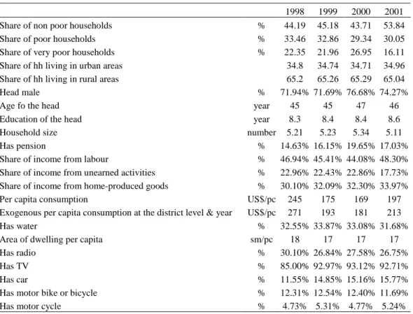
Table 1 presents descriptive statistics for the household characteristics and welfare condition on the whole sample (Table 1).

Table 1: Household Characteristics and Welfare Conditions

1998 1999 2000 2001 Share of non poor households % 44.19 45.18 43.71 53.84 Share of poor households % 33.46 32.86 29.34 30.05 Share of very poor households % 22.35 21.96 26.95 16.11 Share of hh living in urban areas 34.8 34.74 34.71 34.96 Share of hh living in rural areas 65.2 65.26 65.29 65.04

Head male % 71.94% 71.69% 76.68% 74.27%

Age fo the head year 45 45 47 46

Education of the head year 8.3 8.4 8.4 8.6 Household size number 5.21 5.23 5.34 5.11 Has pension % 14.63% 16.15% 19.65% 17.03% Share of income from labour % 46.94% 45.41% 44.08% 48.30% Share of income from unearned activities % 22.96% 22.43% 22.86% 17.73% Share of income from home-produced goods % 30.10% 32.09% 32.30% 33.97% Per capita consumption US$/pc 245 175 169 197 Exogenous per capita consumption at the district level & year US$/pc 271 193 181 213

Has water % 32.55% 33.87% 33.08% 31.68%

Area of dwelling per capita sm/pc 18 17 17 17

Has radio % 30.10% 26.84% 27.58% 26.75%

Has TV % 85.00% 92.97% 93.12% 92.71%

Has car % 11.55% 14.85% 15.16% 15.77%

Has motor bike or bicycle % 12.31% 12.54% 12.40% 11.69% Has motor cycle % 4.73% 5.31% 4.77% 5.24%

Source: Author’s computation based on Kyrgyz HBS 1998-2001

The table indicates that the average age of the family head is larger in non-poor households compared to the poorer ones. The mean years of education of the head does not vary among the period and is, on average, the same for poor and non-poor households (9 and 8 years respectively). However, when looking at rural and urban households, we can see that rural household’s heads tend to be older in rural areas compared to urban ones.

In addition, larger households in term of number of members are poorer families and live in rural areas. The household size remains constant between urban households in all periods but in 2001 decreases slightly among rural households.

At the national level, in 1998, income from labour and entrepreneurial activities constitute 46% of the total household’s income. The share of income from agriculture activities (and home-produced goods) accounted only for 30%. In 2001, we observe a slightly increase in both the share of income from labour and agriculture activities and, at the same time, a decrease of income from unearned activities and disinvestments. Although income shares, during the same period, do not seem to be different between poor and non-poor households, when looking at the rural and urban households we observe that the share of household income deriving from agriculture activities is higher for rural households, accounting for almost a half of total income in 2001. Urban households rely predominantly on income from the labour market (between 73 and 75% in all the periods).

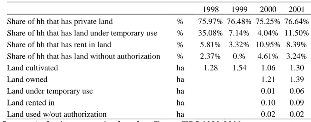
Table 2 summarizes households’ land market participation. Since 1991, the Kyrgyz Republic’s original 470 collective and state farms have been divided into 869 cooperatives and other forms of still- collectivized agriculture, and 29,873 family farms and small-group farms.

Table 2: Land Market Participation

1998 1999 2000 2001 Share of hh that has private land % 75.97% 76.48% 75.25% 76.64% Share of hh that has land under temporary use % 35.08% 7.14% 4.04% 11.50% Share of hh that has rent in land % 5.81% 3.32% 10.95% 8.39% Share of hh that has land without authorization % 2.37% 0.% 4.61% 3.24% Land cultivated ha 1.28 1.54 1.06 1.30

Land owned ha 1.21 1.39

Land under temporary use ha 0.01 0.06

Land rented in ha 0.10 0.09

Land used w/out authorization ha 0.02 0.02

Source: Author’s computation based on Kyrgyz HBS 1998-2001

The percentage of households who own land is about 76% in 1998 and does not seem to change in the whole period. Conversely, the share of households who hold land under temporary use decreases consistently from 35% in 1998 to 11% in 2001. At the same time, the share of households that rents in land increases from 5.81% in 1998 to 8.39% in 2001. The decrease observed from 2000 to 2001 is due to the contemporary increase of land under temporary use during the same years. The percentage of households that use land without authorization is, in the entire period, around 3%. Poor households seem to have higher probability to own land compared to the non-poor. They were the beneficiaries of land reform. The share of poor households that owns land is, on average in the entire period, around 80%. Except for 1999, it seems that richer households prefer to rent in land. Preliminary evidence suggests that Kyrgyz farmers are beginning to participate in the newly emerging land market. Households cultivated, on average, 1.28 ha of land. The amount has been, to some extent, stable in the whole period. The mean area rented amounts to 1.21 ha in 2000 and 1.39 in 20013.

At the beginning of the privatization process, poorer households cultivated 4.5 times less land than richer households. The hectares of land cultivated by poor households remained stable during the four years but the difference is that the total amount of land cultivated by richer household has decreased, especially between 1999 and 2000. Poor households own half the size of land of richer households. The mean size of the holding in 2000 was 1.75 ha, and 0.79 ha for non-poor and poor households respectively. In 2001 it slightly increased for non-poor households to 1.97 ha and decreased for poor ones to 0.71 ha. Households, both non-poor and poor, rent on average a small parcel of land. In 2000, the mean plot of land rented was 0.21 ha for richer households and 0.02 ha for poorer ones.

3

This data is not available in 1998 and 1999, whereas in the 2000 and 2001 surveys the land section is at the plot level. Therefore, the amount of land owned, rented in, temporarily used and used without authorization has been calculated.

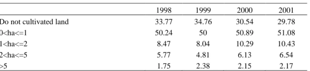
Table 3 presents the main characteristics of the households in the four years according to size classes of cultivated land. The size classes are defined according to ascending size of cultivated land in arable land equivalent4, except for the first class that includes all households that do not cultivate any land.

Table 3: Share of Households that Cultivates Land

1998 1999 2000 2001 Do not cultivated land 33.77 34.76 30.54 29.78 0<ha<=1 50.24 50 50.89 51.08 1<ha<=2 8.47 8.04 10.29 10.43 2<ha<=5 5.77 4.81 6.13 6.54

>5 1.75 2.38 2.15 2.17

Source: Author’s computation based on Kyrgyz HBS 1998-2001

Agriculture plays a central role in the lives of the rural population: in 2001 and on average in the whole period, 70% of households cultivate some land. Out of 70%, in 2001, 50% of the households cultivate, on average, between 0 and 1 ha of land. 10% cultivate between 1 and 2 ha, 6.5% cultivate between 2 and 5 ha of land and the remaining 2% cultivate more than 5 ha of land.

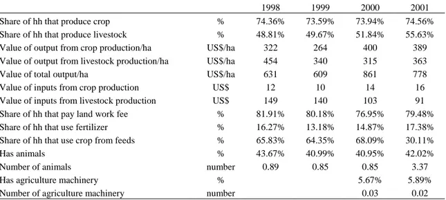
The value of output from crop production per hectare of arable equivalent has decreased significantly from 1998 to 1999 and then considerably increased from 1999 to 2000 (Table 4). The value of output from livestock per hectare of arable equivalent production seems to exhibit a U-shape pattern. It has decreased from 1998 to 2000 and then increased again from 2000 to 2001. Poor households face higher level of output from crop production, whereas richer households obtained a larger part of production from livestock production. This is true for the entire period even though stabilization of the value is observed in 2000 and 2001 after the crisis undergone by the country, and, in particular, by the agriculture sector, in 1999.

4

Different types of land have been reduced to arable equivalent by scaling by appropriate factors. The following weights have been applied to the different type of land: 0.6 to haymaking meadows and pasture land; 2 to orchards. The area under potatoes cultivation, the garden plot, the area under cereals, industrial crop, flowers, crops for fodder have been equalized to arable land.

Table 4: Agriculture Endowment and Profitability

1998 1999 2000 2001 Share of hh that produce crop % 74.36% 73.59% 73.94% 74.56% Share of hh that produce livestock % 48.81% 49.67% 51.84% 55.63% Value of output from crop production/ha US$/ha 322 264 400 389 Value of output from livestock production/ha US$/ha 454 340 315 363 Value of total output/ha US$/ha 631 609 861 778 Value of inputs from crop production US$ 12 10 14 16 Value of inputs from livestock production US$ 149 140 103 91 Share of hh that pay land work fee % 81.91% 80.18% 76.95% 79.48% Share of hh that use fertilizer % 16.27% 13.18% 14.87% 17.38% Share of hh that use crop from feeds % 65.83% 64.35% 68.09% 30.11% Has animals % 43.67% 40.99% 40.95% 42.02% Number of animals number 0.89 0.85 0.85 3.37

Has agriculture machinery % 5.67% 5.89%

Number of agriculture machinery number 0.03 0.02

Source: Author’s computation based on Kyrgyz HBS 1998-2001

Input value is higher in livestock production compared to crop production. Inputs from livestock production account for 20% of total output per hectare in 1998. In 2001, the value of input from livestock production decreased compared to the value of total output5.

The share of households that own agriculture machinery is very low: 5.89% in 20016. The percentage is lower when comparing poor and non-poor households. In Kyrgyz, collective and state farms concentrate more than 80% of all agricultural equipment including tractors and harvesters. This makes smaller farms dependent on larger ones. This phenomenon can be evidenced looking at the share of households that pay land work fee (that can be considered as a proxy of the rental for agriculture machinery): 80% of households in 2001 paid land work fee. This share is, on average, of poor households. Therefore, private farms have higher expenses on renting equipment and other services. Their performance may thus be highly affected, given the high share of households that have to use agricultural equipment and other means of production that remained in collective and state farms.

3.2 Estimation Strategy and methodology

In order to outline the model for the empirical testing, consider farm revenue from agriculture production (v_it) as composed of a systematic part (Q_it) and a stochastic part (y_it).

it it it

v = y Q (3.1)

5 _{It has not been possible to calculate the total households’ profit because of the lack of information} regarding the salary of hired worker and the time spent, for each household member, in on-farm activities.

Taking the logarithm of both sides of (1) yields:

logv_it =logy_it +logQ_it (3.2) The variation of the systematic component (Q_it) can be explained by a production function, describing how output varies across farms and over time as function of the inputs used in production plus a certain number of household characteristics (“shifters” such as: age and education of the head, household size, animals and agriculture machinery ownership). For simplicity and in order to make the notation less cumbersome, the shifters will be omitted from the equation.

1

log log log log

J it it j jit it j Q y

α

X y = + =

∑

+ (3.3)

where j=1...J denotes the inputs used in production. Therefore:

logy_it =ε_it = +v_i u_it

The stochastic term can be decomposed into two components: the first, v_i, refers to the variability across farms (cross sectional variation), and the second, u_it, captures how much of the variance is due to the variability within farm (time series variation).

We assume that farmers cultivate their endowment. They pay a fix cost c for each unit of land cultivated (the costs include both investment in land improvement and maintenance costs).

For simplicity all factors are fixed except land. We assume that the stochastic part of the revenue is distributed around the entry value (persistence)

The value matching condition will be:

1 1 1 '( ) * 1 '( ) y c Ay f q with q q c y f q β δ δ β β = − ≤ ⇒ ₌ − (3.4)

The stochastic component of the revenue can be re-written as follow:

1 1

log log *

log log log log '( ) 1 y y v y

β

c f q v

β

= + = + − + − Equation (3.3) becomes:

log log log ( , ) log * log log ( , ) ( , )

Q y Q x q y v

Q Q x q g

σ

c v

+ = + +

⇒ _{= + +} (3.5)

where x denotes any shifter. For the case of a Cobb-Douglas production function, in particular, γ α_x Bq x q Q( , )= (3.6)

The systematic and the stochastic part of the revenue will be, respectively:

logQ=logB+

α

logq+

γ

logz and (3.7)

1 1

log log *

log log (1 ) log log 1

where log log

y y v B c q z v B B

β

_α

_γ

β

α

= + = + + + − + + − = +

Substituting into equation (3.4), we obtain:

1 1

log( ) log log log log 1

yQ

β

c q

α

v

β

= + + − +

−

Note that on the basis of this equation, we can formulate three specific predictions: a. a positive coefficient not significantly different from one for the

1

β

β

− variable

b. a positive coefficient, again not significantly different from one for the land variable

c. a negative coefficient for land elasticity

α

Also this coefficient should not significantly differ from one. However since we cannot estimate

α

for each farm, we can use the other factors and shifters to measure

α

-differences across farms and times. This implies that we should expect negative coefficients for factors or shifters that are complement to land and positive for substitutes.

3.3 Econometric results

In order to test empirically the equation developed above we have estimated a set of random effect linear regressions on the logarithm of the value of the revenue (from crop and livestock production). Tables 5-8 summarize the results of the regressions.

We have used the entire period 1998-2001 and have performed, in Table 5, a random effect linear regression for the households with non-negative revenue on the unbalanced panel. Table 6 shows the same results for the unbalanced panel of the households that rent in land (tenants).

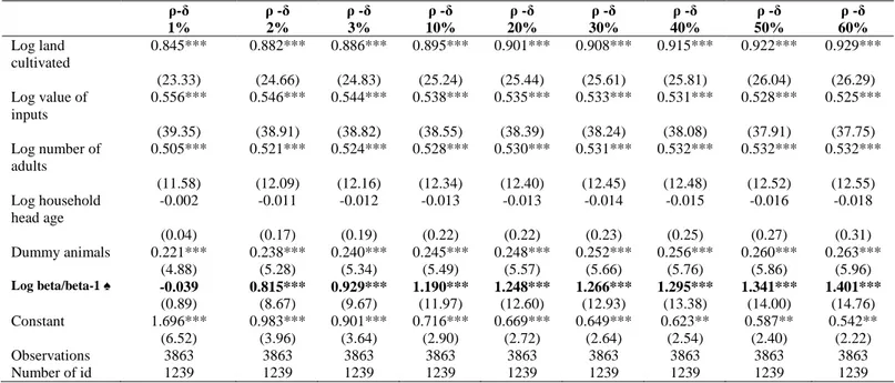
Table 5: Random Effect Linear Regression: Total Revenue Unbalanced panel 1998-2001 ρ-δ 1% ρ -δ 2% ρ -δ 3% ρ -δ 10% ρ -δ 20% ρ -δ 30% ρ -δ 40% ρ -δ 50% ρ -δ 60% Log land cultivated 0.845*** 0.882*** 0.886*** 0.895*** 0.901*** 0.908*** 0.915*** 0.922*** 0.929*** (23.33) (24.66) (24.83) (25.24) (25.44) (25.61) (25.81) (26.04) (26.29) Log value of inputs 0.556*** 0.546*** 0.544*** 0.538*** 0.535*** 0.533*** 0.531*** 0.528*** 0.525*** (39.35) (38.91) (38.82) (38.55) (38.39) (38.24) (38.08) (37.91) (37.75) Log number of adults 0.505*** 0.521*** 0.524*** 0.528*** 0.530*** 0.531*** 0.532*** 0.532*** 0.532*** (11.58) (12.09) (12.16) (12.34) (12.40) (12.45) (12.48) (12.52) (12.55) Log household head age -0.002 -0.011 -0.012 -0.013 -0.013 -0.014 -0.015 -0.016 -0.018 (0.04) (0.17) (0.19) (0.22) (0.22) (0.23) (0.25) (0.27) (0.31) Dummy animals 0.221*** 0.238*** 0.240*** 0.245*** 0.248*** 0.252*** 0.256*** 0.260*** 0.263*** (4.88) (5.28) (5.34) (5.49) (5.57) (5.66) (5.76) (5.86) (5.96) Log beta/beta-1 ♠ -0.039 0.815*** 0.929*** 1.190*** 1.248*** 1.266*** 1.295*** 1.341*** 1.401*** (0.89) (8.67) (9.67) (11.97) (12.60) (12.93) (13.38) (14.00) (14.76) Constant 1.696*** 0.983*** 0.901*** 0.716*** 0.669*** 0.649*** 0.623** 0.587** 0.542** (6.52) (3.96) (3.64) (2.90) (2.72) (2.64) (2.54) (2.40) (2.22) Observations 3863 3863 3863 3863 3863 3863 3863 3863 3863 Number of id 1239 1239 1239 1239 1239 1239 1239 1239 1239

Source: Author’s computation based on Kyrgyz HBS 1998-2001

Table 6: Random Effect Linear Regression: Total Revenue Unbalanced panel of Tenants: 1998-2001 ρ -δ 1% ρ -δ 2% ρ -δ 3% ρ -δ 10%

Log land cultivated 0.642*** 0.664*** 0.666*** 0.671*** (5.53) (5.76) (5.78) (5.83) Log value of inputs 0.741*** 0.728*** 0.727*** 0.724***

(11.93) (11.78) (11.78) (11.77) Log number of adults 0.554*** 0.565*** 0.564*** 0.561***

(3.41) (3.53) (3.53) (3.54) Log household head

age -0.438* -0.419* -0.417* -0.410* (1.78) (1.70) (1.69) (1.67) Dummy animals 0.118 0.138 0.140 0.145 (0.74) (0.88) (0.89) (0.93) Log beta/beta-1 ♠ -0.021 1.000** 1.065** 1.252** (0.08) (2.07) (2.19) (2.54) Constant 2.762** 1.882* 1.829* 1.670 (2.44) (1.83) (1.78) (1.62) Observations 278 278 278 278 Number of id 230 230 230 230

♠ We use variance of total revenue, because we assume that total revenue, v= yQ, so that

logv=logy+logQ and var(log )v =var(log )y since log Q is assumed non stochastic

Source: Author’s computation based on Kyrgyz HBS 1998-2001

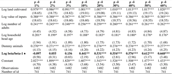
A second set of regressions is presented in Tables 7 and 8. Although our data cover the period 1998-2001, we have restricted the analysis to the last two years because we had better data for this sample. In particular, Table 7 uses the balanced panel and summarizes the results for the households with non-negative revenue. As before, in Table 8 we repeat the same analysis but restricting the sample to the tenants.

Table 7: Random Effect Linear Regression: Total Revenue Balanced panel 2000-2001 ρ -δ 1% ρ -δ 2% ρ -δ 3% ρ -δ 10% ρ -δ 20% ρ -δ 30% ρ -δ 40% ρ -δ 50% ρ -δ 60%

Log land cultivated 0.979*** 0.986*** 0.991*** 1.001*** 1.007*** 1.010*** 1.013*** 1.017*** 1.020*** (18.65) (18.75) (18.82) (19.01) (19.08) (19.11) (19.13) (19.17) (19.24) Log value of inputs 0.388*** 0.388*** 0.387*** 0.387*** 0.386*** 0.386*** 0.386*** 0.385*** 0.385***

(18.63) (18.61) (18.60) (18.60) (18.59) (18.57) (18.56) (18.55) (18.55) Log number of adults 0.241*** 0.245*** 0.248*** 0.256*** 0.259*** 0.260*** 0.261*** 0.261*** 0.262*** (4.45) (4.52) (4.58) (4.73) (4.79) (4.81) (4.83) (4.84) (4.87) Log household head age 0.201* 0.199* 0.197* 0.188* 0.183* 0.181* 0.180* 0.178* 0.176* (1.94) (1.91) (1.89) (1.80) (1.75) (1.73) (1.72) (1.70) (1.68) Dummy animals 0.270*** 0.271*** 0.272*** 0.275*** 0.276*** 0.276*** 0.276*** 0.277*** 0.277*** (4.13) (4.15) (4.16) (4.20) (4.22) (4.23) (4.23) (4.24) (4.25) Log beta/beta-1 ♠ -0.097 0.055 0.156 0.441** 0.531*** 0.554*** 0.576*** 0.612*** 0.668*** (0.58) (0.31) (0.83) (2.19) (2.65) (2.81) (2.96) (3.17) (3.48) Constant 2.027*** 1.899*** 1.820*** 1.607*** 1.543*** 1.526*** 1.508*** 1.477*** 1.433*** (4.70) (4.38) (4.18) (3.68) (3.54) (3.50) (3.47) (3.40) (3.30) Observations 1482 1482 1482 1482 1482 1482 1482 1482 1482 Number of id 741 741 741 741 741 741 741 741 741

♠ We use variance of total revenue, because we assume that total revenue, v= yQ, so that

logv=logy+logQ and var(log )v =var(log )y since log Q is assumed non stochastic

Source: Author’s computation based on Kyrgyz HBS 1998-2001

Table 8: Random Effect Linear Regression: Total Revenue Unbalanced panel for Tenants 2000-2001 ρ -δ 1% ρ -δ 2% ρ -δ 3% ρ -δ 10%

Log land cultivated 0.614*** 0.651*** 0.651*** 0.650*** (4.45) (4.76) (4.76) (4.75) Log value of inputs 0.627*** 0.595*** 0.595*** 0.597***

(8.81) (8.45) (8.44) (8.47) Log number of adults 0.536*** 0.546*** 0.546*** 0.546***

(3.51) (3.67) (3.67) (3.66) Log household head

age 0.041 0.054 0.054 0.053 (0.16) (0.21) (0.21) (0.21) Dummy animals -0.069 -0.020 -0.019 -0.022 (0.44) (0.13) (0.13) (0.14) Log beta/beta-1 ♠ 0.805* 2.495*** 2.501*** 2.420*** (1.66) (3.12) (3.12) (3.04) Constant -0.115 -0.277 -0.281 -0.225 (0.08) (0.23) (0.23) (0.19) Observations 160 160 160 160 Number of id 114 114 114 114

♠ We use variance of total revenue, because we assume that total revenue, v= yQ, so that logv=logy+logQ and var(log )v =var(log )y since log Q is assumed non stochastic

Source: Author’s computation based on Kyrgyz HBS 1998-2001

In all the regressions, the dependent variable is the logarithm of the total revenue (from crop and livestock production). The set of dependent variables (all

measured in logarithms, includes: t the age of family head, the amount of land cultivated, the value of total inputs in production, the number of adults as a proxy of labour input, a dummy for animal ownership and the variable that reflects uncertainty,

that is, the logarithm of 1

β

β

− _.

In each table different regressions have been run by varying the value of

β

, and, therefore 1

β

β

− _{. For each regression we have used a different percentage (from 1} to 60%) of the difference between the discount rate,

ρ

, and the parameter δ of the beta equation. This difference summarizes the percentage growth of farm revenue that the holder of the option is foregoing, in order to keep alive the option to develop land. For example, a value of 10% of the difference

ρ δ

− means that, in order to keep his option to develop land in the future, the owner of the land is giving up a 10% increase of the revenue that he could earn by developing additional land.

We find, in all regressions, that total revenue is positively related to the amount of land cultivated, input use, and the number of adults, that can be used as a proxy for family labour. On the whole, the estimates seem to corroborate the profit maximization model, thereby suggesting that farmers maybe able to choose their investment with a certain continuity. The age of the household head does not seem to affect the revenue. If markets were perfect, household size and land endowment should not affect production decisions. However, there is a common consensus that points towards imperfections in land and labour markets (Holden et al., 2001) in the rural sector where there is a significant presence of inputs endowment.

As survey information on the number of animals owned is unreliable, we constructed a dummy variable to identify whether a household owned animals. The variable is significant and positively related to revenue.

The coefficient of the variable 1

β

β

− _{is positive and significant in most of the} regressions starting from a level of 2% of the rate of growth of the revenue. When the analysis is restricted to the balanced panel 2000-2001 (Table 7) we need a higher percentage (20%) of the revenue in order to find the coefficient significantly different from zero. Except for table 8, in all the regressions, a lower value of the growth rate of the revenue (1%) makes the coefficient of the beta variable non significant. The value of the coefficient, on the other hand, is not significantly different from 1 or tends asymptotically to 1 in all regressions, thereby validating the theoretical model (Figure 1).

Figure 1

Relation between (ρ-δ) and the coefficients from the regressions on the total revenue

-0.2 0 0.2 0.4 0.6 0.8 1 1.2 0% 10% 20% 30% 40% 50% 60% 70% ρ-δ c o e ff ic ie n ts

Coeff. log land cultivated Coeff. Log beta/beta-1

Source: Author’s computation based on Kyrgyz HBS 1998-2001

The same conclusion can be drawn for the coefficient of the variable of land cultivated. In all the regressions it is positive, non significantly different from 1 at the 1% confidence level.

4. CONCLUSIONS

The issue of irreversibility, uncertainty and environmental policy has been largely discussed in the last three decades. Starting from the pioneering paper of Arrow and Fisher (1974), the concept of option value or quasi-option value has been extended by several authors (Conrad, 1980; Hanemann, 1989; Krutilla and Fisher, 1975; Dixit and Pindyck, 1994).

In this study we have extended the analysis of real option value to the case of agriculture land development. This topic is of particular importance especially in Eastern European countries that have experienced a privatization process in the last 10 years.

In this context of large uncertainty about institutional and economical changes, the decision to develop new land, in the agriculture sector, remains a key question for every farmer. The remaining legal restrictions in the sale market or the presence of high transaction costs in the rental market suggest that a better strategy could be to wait before entering any investment in land development.

The results of the model are the following. Both in the case of continuous and discontinuous supply of land and when the hypothesis of decreasing return to scale holds, the relation between the threshold value of revenue per hectare and the amount of land cultivated is positive. The direct conclusion is, in both cases, that uncertainty increases the value of the threshold. The relation between the threshold and the amount of land owned, that is, the size of the holding is positive in the case of continuous supply of land and negative when there is discontinuous supply of land. The direct

consequence is that, in the first case, smaller farms will be more willing to rent land and exercise the option where, in the second case, larger farms will exercise first. This result tends to corroborate the evidence that happened in EEC and FSU. When distribution of land was chosen, therefore when there was a “continuous supply” of land, small farms developed first. In the case of restitution, land was available in larger quantity, larger farms developed first, and contributed to create large cooperative.

Future interesting issues concerning the application of real option value technique to land development are the introduction, in the theoretical model, of other factors affecting the decision to develop land. Variables related to labour and credit markets can be introduced in the model in order to verify changes in the sign and magnitude of the option value of land development.