Al Collegio dei Docenti della Scuola di Dottorato in Scienze Economiche e Aziendali
Università della Calabria
Valutazione della Tesi di Dottorato “Long-run export elasticities for industrial countries, 1990-2012",
dottoranda Alessia Via.
Alessia Via presenta una tesi di Dottorato dal titolo “Long-run export elasticities for industrial countries, 1990-2012".
La stima delle elasticità degli scambi internazionali rispetto ai prezzi relativi è uno dei temi più importanti, controversi e affascinanti dell'economia internazionale.
Il tema é di grande importanza e attualità, poichè dai valori di queste elasticità dipende la performance di diversi regimi di tassi di cambio; in particolare, la stessa sopravvivenza dell'area euro dipende dall'entità degli aggiustamenti in termini di prezzi relativi, e quindi di costi del lavoro, necessari per ridurre gli squilibri degli scambi con l'estero all'interno dell'area euro, che sono probabilmente la causa di fondo della crisi dell'euro. Il tema é controverso, poiché le stime ottenute per queste elasticità sono fortemente discordanti, e spesso in contrasto con le esperienze concrete di tanti paesi. Addirittura, fra gli anni 20 e gli anni settanta del secolo scorso emerse fra gli studiosi di economia internazionale una frattura fra "elasticity pessimists" ed "elasticity optimists", che ebbe il suo momento di massima contrapposizione con la proposizione negli anni settanta di un "approccio monetario all'analisi della bilancia dei pagamenti", che, rifiutando in blocco i risultati di tante stime econometriche, si basava sul postulato di valori infinitamente grandi delle elasticità degli scambi internazionali rispetto ai prezzi relativi (generalizzazione dell'ipotesi del "piccolo paese"). Il fatto che gli impegni richiesti ai paesi che hanno aderito all'Unione monetaria europea riguardino i saldi di finanza pubblica, ma non la dinamica del costo del lavoro, potrebbe forse essere interpretata come una implicita accettazione dell'approccio monetario alle bilance dei pagamenti.
La tesi di Dottorato di Alessia Via fornisce un contributo interessante su questo argomento. Nel primo capitolo viene presentato il framework teorico in cui il lavoro si colloca. Il secondo capitolo presenta alcuni dei modelli econometrici più utilizzati per la stime delle elasticità-prezzo degli scambi internazionali. Il terzo capitolo illustra i risultati delle stime econometriche ottenute per Italia, Germania, Francia, Stati Uniti, Giappone, Regno Unito e Cina, con riferimento al periodo 1990-2012. La tesi, accanto alle stime prodotte utilizzando il VECM, contiene anche un'applicazione della metodologia dei panel non-stazionari, ovviando così al problema di avere stime puntuali per singolo paese che non permettevano di fare un confronto significativo tra tutti i paesi sotto indagine e di capirne le dinamiche temporali; sono state inoltre prese in considerazione diverse variabili di controllo.
La valutazione complessiva sulla tesi é positiva.
Università della Calabria, 08 ottobre 2013
LMr 田嶋Hl l 潰し1人Luu汎\
雪,
UNI VERSI TADELLACALABRI A Di par t i ment odi Ec onomi aeSt at i s t i c a
Sc uol adi Dot t or at o
i nSc i enz eEc onomi c heeAz i endal i
I ndir iz z oEc onomic o
CI CLOXXV
Long−r unExpor t Elas t ic it ies f br I ndus t r ialCount r ies ,1990−2012
Se請Or eSc ient inc oDis c iplinar eSECS−P/01
Di r et t or e: Super vis or e: Tut or : Ch.moPr of Pat hz iaOr dine
T、LJ ,L_−
/Ch諺:岩霊場
Ch・mOPr of Mar iar os ar iaAgos t ino回国田園
D0億Or ando:Dot t .s s aAles s iaVia
UNIVERSITÀ DELLA CALABRIA
Dipartimento di Economia e Statistica
Scuola di Dottorato
in Scienze Economiche e Aziendali
Indirizzo Economico
CICLO XXV
Long-run Export Elasticities for Industrial Countries, 1990-2012
Settore Scientifico Disciplinare SECS – P/01
Direttore: Ch.mo Prof. Patrizia Ordine
Supervisore: Ch.mo Prof. Antonio Aquino
Tutor: Ch.mo Prof. Mariarosaria Agostino
1 Thesis submitted in fulfilment of the requirements for the degree of
Ph.D. in Applied Economics and Managerial Decisions Settore Scientifico Disciplinare: SECS-P/01
Acknowledgments ………4
Abstract………...……….5
Sintesi………..…………....5
CHAPTER 1:INTRODUCTION 1. Preface……….………...………6
2. Objectives and contributions ………...………...………..6
3. Outline ……….………..………..9
CHAPTER 2:LITERATURE REVIEW 1. Introduction ……….………...………… 11
2. International trade elasticities: concept and definition ...….………..……… 11
2.1. The historical background………..………. 12
2.1.1. The theoretical literature………...………… 12
2.1.2. The Imperfect Substitutes model ………...………… 13
2.1.3. Relative price and exchange rates: a complete pass-through ………… 17
2.1.4. The development of time series econometrics……… 17
2.1.5. The empirical model for trade elasticities ……… 18
3. Estimating time series: different approaches and empirical contributions for trade elasticities………...……… 19
3.1. Distributed-Lag and Autoregressive Models approach……… .. 19
2
3.1.2. The ARDL model……….……… 22
3.1.3. Estimation issues……….……… 22
3.1.4. Empirical contributions……….……… 23
3.2. Phillips’ Fully Modified Estimator approach……….…… 26
3.3. DOLS approach……….……….………… 28
3.4. Cointegration and Error Correction Model approach……… 30
3.4.1. Empirical contributions ……….……… 35
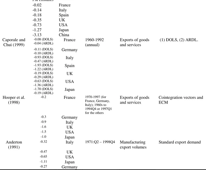
4. Final remarks and summary table……….………… 38
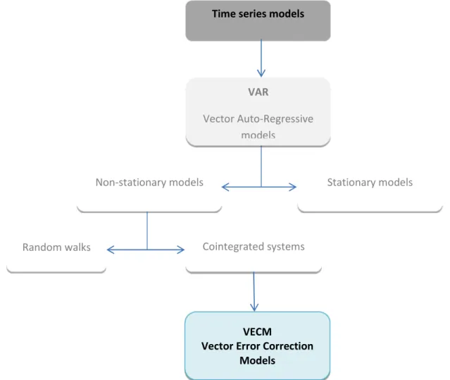
CHAPTER 3:ESTIMATING EXPORT ELASTICITIES USING A VECTOR ERROR CORRECTION MODEL 1. Introduction ………..……….… 42
2. The Marshall-Lerner condition and the J-curve effect ………. 42
3. Empirical background settings………..………. 44
3.1. Introduction………..……… 44
3.2. Simultaneous equation models ………. 45
3.3. VAR models ……… 46
3.4. VECM analysis……… 47
3.4.1. Advantages of using VECMs……… 50
4. A VECM analysis for Italy, Germany, France, USA, Japan, UK and China ……… 51
4.1. Outline……… 51
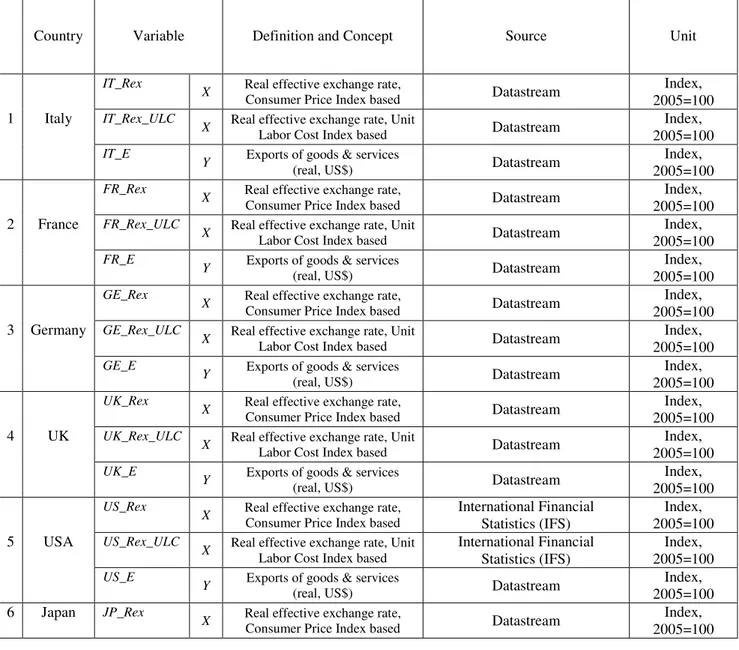
4.2. Data………... 52
4.3. Variables……… 52
5. Estimates………...54
5.1. Introduction………. 54
5.2. Export elasticity estimates for Italy ……… 55
3
5.2.2. Johansen cointegration test……….. 59
5.2.3. Estimates………61
5.3. Export elasticity estimates for Germany, France, USA, Japan, UK and China … 64 6. Discussion of the results………...66
6.1. Evidence for the Marshall-Lerner condition……… 67
6.2. Final remarks………..……… 69
CHAPTER 4:ESTIMATING EXPORT PRICE ELASTICITIES USING NON-STATIONARY PANEL MODELS. EVIDENCE FROM A SAMPLE OF COUNTRIES. 1. Introduction………..……….……….72
2. Empirical setting and data………...………….……….……….…73
3. Econometric methodology………….……..……….……… 74
3.1. Stationarity and cointegration tests ……….………..…………..………...75
4. Panel estimation of the long-run relationship…...………..………77
4.1. Pooled Mean Group (PMG) estimation ……..……….………..79
4.2. Mean Group (MG) estimation……….………...………..…………...81
4.3 Testing for structural breaks………..………..………85
5. Final remarks ……….89
FORTHCOMING RESEARCH……….……….……91
CONCLUSIONS……….………92
References…..…………96
4 Acknowledgements
My Doctoral Thesis was inspired and supervised by Professor Antonio Aquino. I am in great debt with him for having made it possible to start and to carry out my research but, most of all, for having made my return to academia, after more than ten years, challenging and stimulating. I cannot possibly express the extent of my gratitude for believing in me when even I didn’t.
It is also a pleasure to formally thank some of those who have generously shared their time, insights and wisdom with me in the past three years: my friend and Professor, Francesco Aiello and my friend and colleague, Graziella Bonanno: thank you. I am very grateful to Professor Mariarosaria Agostino for all her helpful critiques, feedbacks and moral support.
A special thanks goes to the Professors and colleagues of the Doctoral School for guiding my studies and for their precious advices.
However, my greatest debt is with my children, my husband, my parents and my whole family without whose encouragement, understanding, patience and absolutely unselfish support, this thesis could not have been written. It is to them that I dedicate my research.
5
LONG-RUN EXPORT ELASTICITIES FOR INDUSTRIAL COUNTRIES
1990-2012
Abstract
External imbalances are a threat for the global economy and disorderly adjustments as well as errors in forecasting the effects of policies can yield strongly negative outcomes. Focusing on export price elasticities, my main purpose is to provide an overall view of the previous research carried out on trade elasticity issues and to analyze the implications of global current account imbalances. Export price elasticities estimated in the previous literature feature a high variability with values ranging from -0.14 to -3.13. Some of these results can be considered controversial with respect to one side of the current debate and cause complexity in their interpretation. I have first applied a cointegration model in an error correction framework to estimate export elasticities covering the period from 1990 to 2012 for countries that represent both surplus and deficit sides of the current debate: Italy, Germany, France, USA, UK, Japan and China. Furthermore, I have used a non-stationary panel technique to take into account both inter-country differences and dynamic variations. Using these estimates, in combination with the prevalent macroeconomic forecasts related to the issue, I have illustrated how variations in exchange rates and incomes can produce effects on exports.
Sintesi
Gli squilibri nei pagamenti internazionali rappresentano una minaccia per l’economia globale. L’obiettivo principale di questo lavoro è fornire una visione complessiva delle ricerche svolte sulle problematiche riguardanti le elasticità del commercio internazionale, ed analizzane le implicazioni per gli squilibri delle bilance commerciali. Per ciò che riguarda le esportazioni, le elasticità dei prezzi stimate nella letteratura presentano una forte variabilità con valori che variano da -0.14 a -3.13. Alcune di queste stime, in particolare, possono essere considerate controverse e sono complesse nella loro interpretazione. Per le stime è stato utilizzato in questa tesi un modello di cointegrazione nell’ambito del Meccanismo di Correzione dell’Errore per stimare le elasticità delle esportazioni per il periodo che va dal 1990 al 2012 per Paesi sia in surplus che in deficit di bilancia dei pagamenti: l’Italia, la Francia, la Germania, gli USA il Regno Unito, il Giappone e la Cina. Successivamente, per arricchire l’analisi con le variazioni nel tempo e nello spazio, è stato implementato un panel non-stazionario. Le stime ottenute sono state utilizzate per illustrare l’entità dell’impatto sulle esportazioni dei diversi paesi delle variazioni dei tassi di cambio.
6
CHAPTER1
INTRODUCTION
1.PREFACE
One of the most important issues in applied International Economics is the effect on trade flows of changes in income and relative prices. The increasing interdependence among countries and their efforts to maximize benefits from international trade makes the import and export demand equation specifications essential not only for forecasting, planning and policy formulation but also for the quantification of welfare gains from trade (Hamori and Yin, 2011). The estimation of income and price elasticities of trade is consequently the main object of several studies on the determinants of imports and exports. Price elasticities are particularly important for estimating the effects of changes of relative prices on trade flows and for determining to which degree they adjust to these changes.
The “elasticities” approach of the econometric specifications has, in fact, always been used in international economics to determine the causes of trade just for its capacity both to explain the past and to forecast and, consequently, plan the future. The main elements of this model are the elasticities of exports and imports with respect to economic activity and to relative prices, and the influence of other factors, including global supply and increased variety and interdependence. Export elasticities, in particular, are often used to show the relative flexibility of certain exporters when facing a loss of competitiveness while the price elasticity of imports reflects consumers’ fidelity to domestic or foreign goods.
All these reasons can only partially explain why the role played by trade elasticities is considered fundamental in translating economic analysis into policy-making.
Given the importance of the issue, economists are interested in understanding how it will evolve in the future and, above all, how empirical models and techniques can improve with respect to the existing literature.
2.OBJECTIVES AND CONTRIBUTIONS
Export elasticity estimation is one of the most important, controversial and intriguing topics in International trade as well as the oldest empirical efforts in economics. According to Goldstein
7
and Khan (1985), there were 42 books and articles by 1957 and Stern et al. (1976) cite 130 articles from the period 1960-1975, which estimate the trade elasticities. Sprinkle and Sawyer (1996) pick up in 1976 and survey approximately 50 articles, which estimate the trade elasticities. Most econometric estimations indicate that price elasticities fall in a range of 0 to –4.0, while income elasticities fall between 0.17 and 4.5. The high variability of trade elasticities estimates suggests that there are still gaps in this research area: in fact, since the values of price elasticities vary considerably, the recent literature questions the effectiveness of real devaluation in affecting exports. The importance and the interest of the issue lies on the fact that performance of the different kind of exchange rate policies and systems depends on the results of these estimations.
In spite of more than 50 years of analyses, the estimation of price and income trade elasticities in the international scenario is still an open and highly significant empirical subject; perhaps, this interest can be addressed, among other factors, to questions that do not achieve a total concurrence of results:
• do exports actually expand after depreciations? If so, by how much?
• can exchange rates alone represent a feasible policy to improve the trade balance?
The topic is controversial because the estimated price elasticities of the last decades are extremely contrasting not only between one another but also with the concrete experience of many countries like Germany. It is true that countries like the USA and Germany both push other countries (i.e. China) to appreciate their currencies but, while the USA are facing deficit issues, Germany cannot say as well: its export market share has increased in recent years, especially towards Asia1.
Something in this context does not figure: or the complaints of the major exporters are without basis, meaning that any sort of exchange rate manipulation is nearly worthless (i.e., exports are not so sensitive to movements in exchange rates at least at an aggregate level) or the elasticities reported by the literature are, for some reason, inexact.
The motivation for this research is, therefore, explained by the extremely important consequences of trade elasticity estimates; my interest arose after reading several articles (and the related issues and studies) on the global imbalances and on how changes in exports are habitually seen as the key for realignments in the international scenarios. This represents the starting point and inspiration of the study: the estimation of trade elasticities. During the course of the study, an
1
8
increasing focus on export functions occurred and, in particular, on long-run export price elasticities. From an economic point of view, the constant complaints about devaluation policies could been seen, indeed, as a signal and could disclose further outcomes useful for the study of international interdependencies and trade patterns; from an empirical point of view, both research articles and reference texts provide alternative methods for deciding on the model structure and this was also a challenging aspect: the over fifty years of econometric development in time series analyses offer different milestones for the building of an appropriate model. Indeed, despite the immense literature, and perhaps, as a consequence of this, there are different approaches and a lack of uniformity not only in the models applied but also in the results of the estimations. This leads to another important consideration: due to the highly relevant use of trade elasticities, if the results of the estimation vary through sample periods, methods and models, other empirical analyses could be useful.
In an attempt to address all the above mentioned issues, the objectives of this research are to:
• review trade elasticity literature both from a theoretical and an empirical perspective;
• identify contradictions and/or discrepancies in the estimates of export price elasticities in the published literature in a comparative framework and for chosen countries;
• describe and apply appropriate models within a time series and non-stationary panel cointegration framework approach;
• summarize, interpret and discuss the elicited results and the techniques used for the estimation in order to address the question of the nexus between weak currencies and improved trade balances.
More specifically, my goal is to assess whether policymakers can exploit the relationship (if any) between exports and policy to weaken the currency and promote growth through competitive devaluations. In this context, after providing an overall view of the previous research carried out on this topic and illustrating the main issues related to it, this thesis complements the existing literature by implementing both time series and panel data techniques for non-stationary series using aggregate trade data.
The novelty of this research is the use of frontier panel techniques to estimate the coefficients of the long-run export price elasticities. This study can be considered relevant because, by estimating long-run export price elasticities and their dynamics over time, it could allow to understand more about the consequences of changes in relative prices, so that policymakers could assess better their interventions and attempt to implement correct adjustments.
9
To sum up, the research contributes to the body of knowledge by:
• summarizing the literature on export elasticities by describing the most established approaches ;
• estimating export price elasticities for seven countries (Italy, Germany, France, UK, USA, Japan and China) over the period 1990-2012 applying different cointegration methods; • addressing the competitive devaluation issue.
3.OUTLINE
This thesis consists of the following three sections. Chapter 2 reviews the literature on different economic and, especially, econometric approaches to the estimation of international export elasticities. This chapter provides a discussion of some of the issues involved in the estimation of the price elasticities of the demand for exports according to the existing literature and its evolution over the years and some results. This is required in order to provide a general and detailed (although not exhaustive) outlook of the body of work.
Chapters 3 outlines the data used and the empirical setting of export elasticities and explains the econometric methodology applied to estimate the long-run export elasticity equation - i.e. the time series cointegration analysis using the vector error correction model (VECM).
In order to provide more robust estimations of long-run export elasticities, Chapter 4 refers to panel data techniques. In particular, it is based on the non-stationary panel pooled mean group (PMG) and the mean group (MG) models. The chapter reports the evidence found when allowing for inter-country and intra-country variations of short and long-run price-elasticity.
The discussion and the interpretation of the results as well as the conclusions of this study are presented in the final sections of the thesis.
10
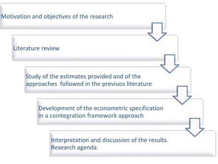
Figure 1.3. Research outline
Motivation and objectives of the research
Literature review
Study of the estimates provided and of the approaches followed in the previuos literature
Development of the econometric specification in a cointegration framework approach
Interpretation and discussion of the results. Research agenda.
11
CHAPTER 2
LITERATUREREVIEW
1.INTRODUCTION
The purpose of this section is twofold:
• to provide an overview of the previous theoretical and empirical literature within the international trade elasticities context;
• to act as a gateway to the methodology and the econometric specification applied in the present analysis.
Some preliminary remarks are necessary before starting.
First of all, in order to provide a fluent overview of the literature, it was decided to analyze the different studies proceeding by the main empirical and theoretical approaches followed and not by a chronological sequence: the existing literature, in fact, is very extensive - covering a period of over fifty years - and arranging the numerous researches by date would have made it very complicated to offer a general and overall outlook of the issue. In addition, taking into account the results of earlier empirical studies – equally important – an emphasis was reserved on the empirical contributions of the recent years.
Secondly, the econometric sophistication of time series goes hand in hand with the development of the international trade elasticities theories. For this reason, they are treated together. Finally, this section is not to be considered exhaustive in including all the methodologies and cases studied up to now but rather it has to be read as a detailed summary which is intended to provide a background to the recent economic developments in times series econometrics and, in particular, in the estimation of international trade elasticities.
2.INTERNATIONAL TRADE ELASTICITIES: CONCEPT AND DEFINITION
Trade elasticities measure the responsiveness of demand or supply to changes in income, prices or other variables. The two main elasticities are the income elasticity and the price elasticity of demand. The income elasticity measures the percentage change in the quantity demanded resulting from a one-percent increase in income with E = elasticity, Q = quantity demanded, I = income and P = relative price (Escaith et al., 2010):
12
The price elasticity measures the percentage change in the quantity demanded resulting from a one-percent increase in relative price:
2.1 The historical background
The estimation of trade elasticities has a very long history from both a theoretical and an empirical point of view. It is nonetheless firm that few papers cover all the issues raised in the econometric literature (Sawyer, Sprinkle, 1996).
2.1.1 The theoretical literature
The forerunner of the great amount of research concerning the estimation of trade elasticities is Orcutt (1950). Beginning with his paper, the large body of literature in this field has involved issues referring not only to how the elasticities are used and how they are determined but also to the development of the econometric specifications. These papers were first surveyed by Stern et al. (1976) and Goldstein and Khan (1985) and, since the 1970s, the literature has continuously evolved, entailing different issues related to trade elasticities.
The theoretical model underlying the estimation of trade elasticities is an imperfect substitutes model, that is, a model in which it is assumed that exports and imports are imperfect substitutes for domestically produced goods. Goldstein and Khan (1985) provide a detailed discussion of this model. In an imperfect substitutes model, the foreign demand for goods and services is determined by three main factors: foreign income, the prices of domestic goods and services, and the prices of goods and services that compete with domestic goods and services in the foreign market. Similarly, the domestic demand for foreign goods and services is determined by the
13
country’s income, the prices of foreign goods and services, and the prices of goods and services that compete with foreign goods and services in the domestic market.
The income elasticity of demand for imports measures to what extent changes in an importing country’s income have an effect on changes in its imports. In the same way, the income elasticity of demand for exports measures to what extent changes in foreign countries’ incomes affect the demand for exports.
Usually import and export elasticities with respect to income are positive, that is: an increase in a country’s income leads it to buy more from foreign countries. An income elasticity of imports or exports that is equal to one implies that imports or exports increase at the same rate as income.
Divergences from this imply long-term imbalances in the global economy. Specifically, an income elasticity for imports greater than one implies that, at the margin, domestic consumers have a stronger preference for foreign goods than for domestic goods. This means that if prices do not adjust, imports increase more than proportionately to income growth. This case is particularly meaningful for countries that, on an international scale, experience a higher income growth rate (nota: emerging economies) since, compared to others, these countries will be encouraged to develop their demand of imports and this may possibly overweigh their exports: specifically, in many East Asian economies in which most of imports are used for re-exports, an increase in exports may entail, to some extent, a similar increase of imports. As a matter of fact, many of the imports into these countries are parts and components or capital goods that are used to assemble goods for re-export to the rest of the world. An exchange rate appreciation that reduces exports will also reduce the demand for imported goods that are used to produce exports (Thorbecke, 2010).
On the other hand, economic theory predicts that the volume of imported goods will decrease, while the volume of exported goods will increase, when the relative prices of a country's products decline, i. e. when its real exchange rate depreciates. The problem is: what happens to the value of exports and imports as a consequence of a country's real exchange rate depreciation? The answer depends upon the size of price elasticities of exports and imports.
2.1.2 The Imperfect Substitutes Model
Since the amount of export (and import) adjustments depends on the sensitivity to price and income variations, it is important to estimate the price and income elasticity of a country’s exports. The theoretical basis of the empirical analysis is the Imperfect Substitutes Model. The basic assumption of the model is that neither exports nor imports are perfect substitutes for domestic products. Such a
14
hypothesis is confirmed by empirical evidence. If domestic and foreign goods were perfect substitutes, a given country would be either an exporter or an importer. Since the world market is characterised by the presence of bilateral trade and the coexistence between imports and domestic production, the hypothesis of perfect substitution can be rejected (Algieri, 2004).
Moreover, a large body of empirical studies (Kravis and Lipsey (1978); Kravis and Lipsey) have shown that price differentials can be surprisingly large for the same product in different countries, as well as between the domestic and export prices of a given product in the same country. In other words, the law of one price (LOP) fails dramatically in practice, even for products that are usually traded in international markets. The LOP states that prices in different parts of the world for a given product should be the same when expressed in a common currency. All this said, the finite price elasticities of demand and supply that the imperfect substitutes models postulates can, therefore, be estimated for traded goods.
The imperfect substitutes model2 (Goldstein and Khan 1985; Hooper and Marquez, 1995) of the home country’s exports to, and imports from, the rest of the world (*) is formalized by a set of equations: Md = γ (Y, PM, P) γ1 , γ3 >0, γ2 < 0 (1) Xd = π(Y* e, PX, P*e) π1 , π3 >0, π2 < 0 (2) Ms = φ[PM* (1+S*), P*] φ1 >0, φ2 < 0 (3) Xs = ξ[PX (1+S), P] ξ1 >0, ξ2 < 0 (4) PM = PX* (1+T)e (5) PM*= PX (1+T*)/e (6) Md=Mse (7) Xd=Xs (8)
The eight equations identify the quantities of imports demanded by the home country (Md), the quantity of exports demanded by the world from the home country (Xd), the quantity of imports supplied by the rest of the world to the home country (Ms), the quantity of the home country exports supplied to the rest of the world (Xs), the prices in domestic currency paid by the importers (PM and PM*) and the prices in domestic currency paid to the exporters (PX and PX*). The level of nominal
2
15
income (Y, Y*), the prices of domestic commodities produced within the regions (P, P*), proportional tariffs (T, T*), subsides to imports and exports (S, S*) and the real exchange rates (e) are the explanatory variables.
Foreign demand for goods and services is determined by three main factors: foreign income, the prices of domestic goods and services, and the prices of goods and services that compete with domestic goods and services in the foreign market.
Similarly, the domestic demand for foreign goods and services is determined by the country’s income, the prices of foreign goods and services, and the prices of goods and services that compete with foreign goods and services in the domestic market.
In the imperfect substitutes model the demand functions for exports and imports describe the quantity demanded as a function of the level of monetary income in the importing country, the imported product’s own price, and the price of domestic substitutes. By considering a logarithmic utility function, the income (γ1 and π1) and price elasticity (γ3 and π3) of substitutes are assumed to be positive, while the price elasticity of the traded product is assumed to be negative (γ2 and π2).
Let us assume the demand function to be homogeneous of degree 0, equation 1 can be written in the following way:
Md= γ (Y/P , PM/ P) γ’1>0, γ’2<0 where
Y/P = real income and
PM/ P = real import price
Considering an n-country model, the symmetry between the demand function for imports and the demand function for exports vanishes. Imports compete, in fact, only with goods produced within the country. Exports compete both with goods produced in the imported country and with exported goods by third countries. The equation 2 is corrected with prices of competing goods. Xd / X*
d = π (P* Xd/P* X*d)
16
The supply functions depend on the prices of exported and domestic goods and on subsidies. The price elasticities of exported and local commodities (φ1 and ξ1) are assumed to be positive, the
price elasticities of substitutes (φ2 and ξ2) are supposed to be negative. The equilibrium conditions are represented by the last two equations. The implicit hypothesis is that prices move in order to equate demand and supply over time.
The imperfect substitutes model, by presenting both demand and supply side equations, allows to identify simultaneous relationships among quantities and prices. Orcutt (1950) and Goldstein and Kahn (1985), have highlighted this characteristic but, nonetheless, a multitude of time series works on export and import equations have considered the supply side only by assumption.
In the early 1990s, the standard methodology to estimate import (Eq. 1) and export demand (Eq. 2) was based on the assumption of an infinite supply-price elasticity for imports and exports (φ1 in Eq. (3) and ξ1 in Eq. (4)). Under this hypothesis, PM and PX were viewed as exogenous and thus estimated by single equations.3
Since the late 1990s, economic researchers have improved more and more their approach to the analysis and have applied cointegration analyzes or Fully-Modified-OLS methodologies to deal with simultaneity problems and to overcome endogeneity and serial correlation biases.
According to the literature examined in this study, therefore, the basic linear specifications for the export (2.1) demand function4 can be expressed as follows:
Log Xt = a + b Log (PX/PXW) t + c Log Yt+ ε t (2.1)
where Xt = volume of exports, PXt = export prices, PXWt = world export price level, Yt = world
income and ε is an error term. The price elasticity is given by b5.
A complete model will include other explanatory variables affecting demand besides income and prices. Houthakker and Magee (1969), for example, include control variables for domestic or
3
If the supply elasticities were instead, less than infinite, the problem would be more difficult because one should either calculate the complete structural system of simultaneous equations or solve the reduced form for quantities and prices as functions of the exogenous variables in the system (Algieri, 2004).
4
The import demand function is: Log Mt = a + b Log (PM/PD)t + c Log Yt+ εt where Mt = volume of imports, PMt = import prices, PDt = domestic price level, Yt = domestic income. The price elasticity is given by b.
5
17
world GDP, to estimate the income elasticity of imports. Recently, Algieri (2011) included an unobserved component (UC) to model the export equation.
2.1.3 Relative prices and exchange rates: a complete pass-through
Thus far, enunciating the classical model provided by the literature, relative prices have always been mentioned as one of the most important variables of the export demand function. At this point, the question that could arise is how relative prices link to exchange rates and why recent models include real exchange rates rather than including (directly) relative prices of exported goods.
A last question to examine when talking about the export concerns, therefore, the relative prices. The main assumption made in this study (and according to the literature) is that there is a complete pass-through between relative prices and real exchange rates: that is, exchange rate fluctuations translate into proportional movements in the domestic price level and, therefore, pass-through is equal to one; this simplification offers the opportunity to gauge the price elasticity estimates using the real effective exchange rates without taking into account other factors that can determine divergent fluctuations and, most of all, without invalidating the estimates.
Exchange rate pass-through literature takes its roots from the aforementioned LOP and the Purchasing Power Parity (PPP) literature6. According to Anaya (2000), when using a 20-year time period, pass-through estimates for most countries are close to one supporting a long-term stable relationship. This kind of relation fits closely the purposes of the present study and, for this reason, the variable actually included in the model will be the real effective exchange rates.
2.1.4 The development of time series econometrics
Since the 1970s, the empirical literature evolved as a consequence of the rapid development of times series econometrics and of the need to consider the idea that trade flows do not respond instantly to changes in relative prices (and also in income and exchange rates). New theoretical and technical outcomes led to a vast number of papers beginning with Stern et al. (1976). Starting from the 1990s until today, the cointegration analysis and all the concepts related to it have become an important frame model.
As a result, the early specifications have experienced over fifty years of econometric sophistication, surveyed in Marquez (Marquez, 2002). In the last years, namely, Marquez (2002) or
6
According to Anaya (2000), the Relative PPP (a weak version of the strong PPP) basically implies that the exchange rate and domestic and foreign price levels move proportionately to each other. Namely, strong version of PPP implies that pt = etpt* while the relative PPP implies pt = α et pt*where α is the real exchange rate or alternatively, is the home
18
Kwack et al. (2007) report some estimates for 8 Asian economies, including Hong Kong, the Philippines, whereas Cheung et al. (2009) estimate Chinese trade elasticities. The new models:
- include differences between short and long run elasticities; - ponder the importance of heterogeneity between traded goods; - study the stability of trade relationships;
- cope with endogeneity issues.
In particular, most of the researchers have tried to reduce endogeneity and this attempt is clear in all this recent (and vast) empirical literature. The effort consists mainly in introducing simultaneous equations and cointegration analysis. The main notion behind the cointegration analysis is that if a linear combination of a set of nonstationary variables (such as those in the import demand model) is stationary, those variables are said to be cointegrated. Indeed, recent developments in econometric literature have shown the non-stationarity of most macro data and this substantially invalidates the OLS, 2SLS and Instrumental Variable techniques results7. The Johansen (1988) Johansen – Juselius cointegration approach (1990) and the Engle – Granger (1987) two step approach have been used more and more to reveal the existence of long-run relationships and, in addition, produce empirical results that are not spurious (Marquez, 1990; Gagnon, 2003; Hooper, Johnson and Marquez, 1998; J.S. Mah, 2000).
2.1.5 The empirical model for trade elasticities
The empirical literature on trade elasticities goes back to at least Kreinin (1967) or Houthakker and Magee (1969) followed by Khan (1974), (1975), Goldstein and Khan (1976), (1978), Wilson and Takacs (1979), Warner and Kreinin (1983), Haynes and Stone (1983), Bahmani-Oskooee (1986), Marquez (1990) and Mah (1993). This plethora of studies of the past have all estimated trade elasticities using the OLS, 2SLS method or Instrumental Variables methods. (Bahmani-Oskooee, Niroomand, 1998).
It is indisputable that the empirical literature is vast and that most of the attention is addressed to the forecasting properties of the estimates. Most econometric estimations indicate that price elasticities fall in a range of 0 to –4.0, while income elasticities fall between 0.17 and 4.58. Since the values of price elasticities vary considerably, the recent literature questions the effectiveness of real devaluation in affecting exports and imports. According to Rose (1990, 1991)
7
When data are nonstationary, inferences based on the standard techniques are no longer valid because they suffer from the “spurious regression” problem, see Bahmani-Oskooee, Niroomand, (1998).
8
Algieri B., (2004), Price and Income Elasticities of Russian Exports, The European Journal of Comparative Economics, Vol. 1, n. 2, 2004, pp. 175-193.
19
and Ostry and Rose (1992), a real depreciation does not impact significantly on the trade balance; Reinhart (1995), Senhadji and Montenegro (1998), Senhadji and Montenegro (1999) provide instead, strong support to the view that depreciations improve the trade balance. It seems that low econometric estimates of price elasticities are unreliable for the purpose of forecasting the effect of a depreciation, and there is a strong presumption that these elasticities lead to a considerable underestimation of its effectiveness (Algieri, 2004).
Modeling the time series behavior of imports and exports is a longstanding issue of economists as well as of econometricians; well along with their research, their main questions concern:
- the type of traded commodity, that is, if it is a homogeneous or a differentiated good;
- the main purpose to which the traded good is designed for, that is, if it is used as a factor of production or as a final product;
- the institutional or legal structure of the environment in which the trade takes place;
- the aim of the modeling analysis, or better, if the intention is to forecast or to test hypotheses;
- the typology of data available, that is, if data are annual, quarterly, monthly, etc.;
- the level of aggregation, that is, if the data are aggregated or disaggregated (and the entity of the disaggregation).
The appropriate model, indeed, relies on all the above mentioned factors.
3. ESTIMATING TIME SERIES: DIFFERENT APPROACHES AND EMPIRICAL CONTRIBUTIONS FOR TRADE ELASTICITIES.
The following sections survey some of the approaches used in the estimation of time series variables. The discussion of each topic will be illustrated by examples and empirical analyzes of selected references.
3.1 Distributed-Lag and Autoregressive Models approach
The estimation of price elasticities is a fundamental part of the econometric analysis of long-run relations. This category of analysis has been the focus of much theoretical and empirical research in economics. Where the variables in the long-run relation of interest are trend stationary,
20
the general practice has been to de-trend the series and to model the de-trended series as stationary distributed lag or autoregressive distributed lag (ARDL) models.
In this section, after a brief illustration of the theoretical issues underlying the distributed-lag and the autoregressive models, the literature overview will examine how the study of trade elasticities of demand has been treated over the years through empirical contributions.
3.1.1 Modeling time lags and long-run relations
Time series data entail a variety of issues related to the fact that the regression model includes not only the current value but also the past values of the variables. The time passing between a cause and its effect is called a lag. The lag may be a specific time (e.g., three months, one year, etc.) but, in many cases, the effects of an economic cause are spread over many months, or even many years. In such cases, we have a distributed lag.
Lags occupy a central role in economics, principally when dealing with aggregate data. When the model includes past values of the regressors (explanatory variables indicated by the X’s), these past values are called lagged values and, therefore, the regression analysis is called
distributed-lag model.
Furthermore, the dynamic behaviour of an economy can reveal itself through a dependence of the current value of an economic variable on its own past values.
When the model includes past values of the dependent variable (Y) among the explanatory variables, it is called an autoregressive model (AR).
We can present a general distributed-lag model with a finite lag of k time periods as:
Yt = α + β0Xt + β1Xt -1 + β2Xt-2 + …+ βkXt-k + ut (2.2)
The coefficient β0is known as the short-run multiplier because it gives the change in the
mean value of Y following the unit change in the X in the same time period. The coefficients β technically can be expressed as the partial derivatives of Y with respect to the X’s9:
=
βkIn this model, after k periods10, we obtain the long-run (or distributed-lag) multiplier:
9
β0 is the partial derivative of Y with respect to Xt, β1 with respect to Xt-1, β2 with respect to Xt-2, and so forth.
10
In the model [2.2], if the explanatory (input) variable X undergoes a one-off unit change (impulse) in some period t, then the immediate impact on Y is given by β0; β1 is the impact on Y after one period, β2 is the impact after two
21
∑ = β0+ β1+ β2+…+ βk = β .
The autoregressive model, instead, is expressed as:
Yt = α + βXt + γYt -1 + ut (2.3)
The autoregressive model actually describes the time path of the dependent variable in relation to its past values and for this reason it is properly known as a dynamic model.
We have to consider that the real world presents a mixture of short-run and long-run adjustments and that these adjustment times are necessary for the dependent variable (in our case, the export/import volumes) to respond to variations in the explanatory variables (relative prices and income). The fact that the dependence of a dependent variable Y on other variables (the X’s) is rarely instantaneous implies that any kind of analysis that involves time series data needs to consider such lapse of time (the so called lag).Very more often, indeed, the effect of a given cause is distributed over a certain period of years. Obviously, for this reason, a closer attention should be paid to the factors which account for distributed lag relationships in order to comprehend the economic theory underlying the nature of the lags and why they occur, first of all.
Generally, there are three main reasons11 that are used to explain why lags occur:
1. psychological reasons, under which we include forces of habit and assumptions on the part of consumers that changes may be only temporary;
2. technological reasons, which include factors such as, in a general case, the lack of knowledge about possible substitutes12;
3. institutional reasons, which include situations in which certain contractual items of expenditure or savings may need to be adjusted before shifts can be made in consumption patterns.
In addition, it is clear that the lapse in reactions can depend on the nature of the variation, that is, if the change is permanent or transitory.
periods, and so on. The final impact on Y is βk and it takes place after k periods. Hence, it takes k periods for the full effects of the impulse to be realized. The sequence of coefficients (β0, β1, β2,…, βk) constitutes the impulse response function of the mapping from Xt to Yt.
11
Nerlove (1958).
12
“Suppose the price of capital relative to labour declines, making substitution of capital for labour economically feasible. Of course, addition of capital takes time (the gestation period). Moreover, if the drop of price is expected to be temporary, firms may not rush to substitute capital for labor, especially if they expect that after the temporary drop the price of capital may increase beyond its previous level. Sometimes, imperfect knowledge also accounts for lags.” (Gujarati, 1995).
22 3.1.2 The ARDL model
As above mentioned, another important case is when we find a dependence of the current value of an economic variable on its own past values. Precisely, models of how decision/policy makers’ expectations are formed, and how they respond to changes in the economy, result in the value of Yt depending on lagged Y’s. So, an alternative way to capture the dynamic component of economic behaviour is to include lagged values of the dependent variable on the right-hand side of the regression together with the other exogenous variables.
In time-series econometric modeling, a dynamic regression will usually include both lagged dependent and independent variables as regressors:
Yt = α0 + α 1Yt-1 + …+ α pYt-p + β0xt + β1xt-1 + … + βk xt-k + εt. (2.4)
The above model is called the Autoregressive Distributed-Lag model, known as ARDL (p;
k). The values of p and k (i.e., how many lags of Y and X will be used) are chosen:
i. on the basis of the statistical significance of the lagged variables;
ii. so that the resulting model is well specified (e.g. it does not suffer from serial correlation).
3.1.3 Estimation issues
A distributed-lag model can be estimated by OLS but this approach leads to a certain number of problems. The first question is related to the length of the lag: even though some economical and/or theoretical considerations must be brought forward on the β’s to avoid estimation problems, there is no way to know a priori what the maximum length of the lag is supposed to be.
Secondly, in time series data, the successive lags tend to be highly correlated (Gujarati, 1995) and this means that we are dealing with multicollinearity and, consequently, with imprecise estimation.
Finally, since results are sensitive to lag-lengths, the search for the optimum lag length can widen the dangerous doors of data mining. Data mining refers to all those activities that have in common, a search over different ways to process or package data econometrically with the purpose of making the model meet certain design criteria (Hoover and Perez, 2000). A ready-mix model does not exist so the general recommendation is to always follow (economic and econometric) theory as a guide for any model building.
23 3.1.4 Empirical contributions
Some studies13 (Bahmani-Goswami, 2004) relied on bilateral trade data to provide strong evidence for the support of positive long-run relation between exchange rate and trade balance. In this sense, the main question is if currency devaluation can be used as a tool to correct trade balances.
When researches follow the traditional approach to estimate import demand and export demand elasticities using aggregate trade data, the problem is that a significant price elasticity with one trading partner could be more than compensated by an insignificant elasticity with another partner yielding an insignificant trade elasticity. This so-called “aggregation bias” problem requires estimating trade elasticities on a different basis. Indeed, a new body of the literature is emerging and it includes analyzes that estimate trade elasticities on bilateral basis.
Ketenci and Uz, (2011) use an ARDL approach to measure the impact of currency devaluation. The assessing of the impact is carried out using the real exchange rate. The model is applied between the EU and its eight major industrial trading partners and, furthermore, its six major trading regions14. The ARDL approach is used to determine whether the dependent and the independent variables are cointegrated. The ARDL approach involves two steps for estimating the long-run relationship:
i. the first step is to examine the existence of long-run relationship among all the variables in an equation;
ii. the second step (applied only if the first step showed a cointegration relationship) is to estimate the short-run and the long-run coefficients of the same equation.
Cointegration relations between the variables of bilateral import and export functions are found to be due not only to the strong relations between trade and real exchange rate but also to
13
“First, some have followed standard textbook prescription by estimating the well-known Marshall-Lerner (ML) condition. The ML condition states that devaluation improves a country’s trade balance if the sum of the price elasticities of that country’s import and export demands is more than unity. Second, some have argued that estimating the ML condition is an indirect approach. Thus, they have adhered to a direct method of establishing a link between the trade balance and exchange rate (as well as other determinants) following a reduced-form modeling approach. In both the first and the second approaches, researchers have mostly used aggregate data and provided mixed results. Recently, a few studies have concentrated on employing disaggregated data. While the disaggregated approach on a bilateral basis is applicable to reduced-form trade-balance models, it cannot be applied to estimate the trade flow elasticities or the ML condition. This is due to the fact that import and export prices are not available on a bilateral basis to obtain bilateral trade volumes. The remedy here is to establish a direct link between a country’s inpayments (value of exports) and outpayments (value of imports) and real exchange rate on a bilateral basis” (Bahmani-Goswami, 2004).
14
Namely: Canada, China, Japan, Norway, Russia, Switzerland, Turkey and the US; the six major regions are: the NMCs, the CEECs, the EFTA, the NAFTA, the ASEAN and the DACs.
24
important relations between EU import and EU income and between EU export and partners’ income. The authors also employ an Error Correction Model (ECM) to provide additional evidence of cointegration among the variables.
Since the data for import and export prices on a bilateral level are not available, the authors cannot estimate trade flow elasticities for determining the Marshall-Lerner (ML) condition in their model. Consequently, they establish a direct link between a country’s value of import and export and real exchange rate on the bilateral basis. The direct method of determining whether currency depreciation is effective in increasing a country’s inpayments from a trading partner consists in considering the export value (or inpayments) and determining how sensitive it is to a change in exchange rate; similarly, they consider import value (or outpayments) and try to determine its sensitivity directly to a change in exchange rate.
The authors employ the Akaike Information Criterion (AIC) in order to select the optimum lag length.
As for the diagnostic statistics, the authors’ models pass all the following tests:
- the Lagrange Multiplier (LM) test to check for the serial correlation among the residuals; - the Jarque-Bera statistic to test the normality of the residuals;
- White’s test to check the heterosckedasticity of the residuals;
- Ramsey RESET test15 to check the functional misspecification of each model.
The long-run elasticities of real exchange rate are used as a proxy of price elasticity for determining the ML condition but they result too low so that the long-run coefficient estimates do not provide any empirical evidence that the ML holds.
For the bilateral export demand equation, the expected positive sign of the long-run real exchange rate elasticities occurs only for three partners (on a total of 14) but it is not significant; in other three cases the real exchange rate is significant but has a negative (unexpected) sign. The negative sign means that there is an adverse effect of the currency depreciation on the bilateral export between the EU and the involved trade partners.
For the bilateral import demand equation, the expected negative sign of the long-run coefficients of the real exchange rate occurs in two cases and the coefficients are significant; this indicates that real depreciation of the euro decrease European imports from the regions involved while in other two cases the adverse effect is observed.
15
25
However, the real exchange rate elasticities are so low that it is impossible to make a conclusion about the effect of currency depreciation on bilateral trade and, according to these results, it actually can be concluded that EU’s imports and exports are insensitive to exchange rate variations16.
Yin and Hamori (2011) have recently analyzed China’s import demand function employing ARDL and Dynamic Ordinary Least Squares (DOLS)17 techniques in the estimation of the long-run coefficients of price and income elasticities. The aim of this study is to resolve the issue of trade balance from the perspective of China’s policy making in the larger context of global imbalances problems.
The import demand model adopted derives from the imperfect substitution theory according to which the demand for real imports is a function of domestic income or GDP and relative price (import price index deflated by an index of domestic prices)18.
The choice of the ARDL is motivated by the authors’ consideration that, according to recent evidence, it possesses desirable small sample properties and can effectively correct for possible endogeneity of explanatory variables; they also include the estimates from DOLS, regarded as one of the most widely used estimators of cointegrating vectors in applied literature.
Before interpreting the estimated import demand equations, the existence of a long-run import demand relationship is analyzed. In order to do so, different bound tests are employed using the Johansen (1991, 1995) approach. Since there is strong evidence of the existence of a long-run relationship among the variables included in the long-run import demand model, they estimate the long-run cointegration relationship (long-run coefficients) for imports using the ARDL and DOLS single equation estimation methods.
The authors employ the Schwarz-Bayesian Information Criterion (SBIC) in order to select the optimum lag length.
The diagnostic tests carried out by the authors are the following: - autocorrelation tests
16
See also Bahmani-Goswami, 2004.
17
See paragraph 3.3 of the current section for the DOLS empirical contributions.
18
The traditional import demand model is expressed as: ln Mt = α0 + α1lnYt + α2 ln RPt + εt, where ln is the natural
logarithmic form and εt is the error term. Mt denotes the volume of imports at time t, Yt denotes real income at time t, and RPt denotes the relative price (the import price index deflated by a GDP deflator) at time t. Generally, the hypothesized values of the coefficients of the explanatory variables are α1> 0 and α2< 0, which represent the income and
26
- the Jarque-Bera statistic to test the normality of the residuals; - heterosckedasticity test of the residuals.
The estimated residuals did not provide any significant evidence of serial correlation, non-normality or heterosckedasticity in the error term.
The DOLS estimates of the relative price coefficient are higher as compared to those from ARDL. Indeed, the estimated coefficients for income and relative price variables were found to be rather different when different estimation techniques were employed.
For what concerns the policy-making implications, they reported the following considerations: first of all, the estimated long-run elasticity is inelastic and approximately within the range of –0.5 to –1. Hence, it appears that China cannot depend on using its exchange rate policies to correct the balance of trade problem. The long-run price elasticity is statistically significant, suggesting that if the growth in inflation in China is related to the import price, then China’s imports will increase (and the trade balance will get worse). Second, the growth in income has a significant and elastic impact on import demand in the long-run.
3.2 Phillips’ Fully Modified Estimator Approach
Senhadji and Montenegro (1999) have conducted a cross-country analysis for a large number of developing and industrial countries of export demand equations to gauge export price and income elasticities. The technique implemented accounts the non-stationarity for the data and is derived from dynamic optimization. In this study, the export demand equation is expressed as follows:
log (xt) = γ0 + γ 1log(xt –1) + γ 2log(pt) + γ3log(gdpxt*) + et (2.5)
where xt is real exports of the home country; pt is the export price of the home country
relative to the price of its competitors; and gdpxt* is the activity variable defined as real GDP minus
real exports of the home country’s trading partners. Thus, this model is close to the standard export demand function except that the income variable is real GDP minus real exports of the trading partners, rather than the trading partners’ GDP. The equation is estimated using both OLS and Phillips’ Fully Modified estimator (FM) The fully modified OLS (FM-OLS) approach originally proposed by Phillips and Hansen (1990) which takes into account the non-stationarity in the data as well as potential endogeneity of the right-hand side variables and autocorrelation of the error term.
27
The FM estimation method is, indeed, an approach to regressions for time series taking advantage of data non-stationarity and cointegrating links between variables. Cointegrating links between variables lead to endogeneity of regressors: the FM estimator is designed to estimate cointegrating relationships by modifying OLS with corrections that take into account of endogeneity and serial correlation.
The long-run price and income elasticities are defined as the short-term price and income elasticities divided by one, minus the coefficient estimate of the lagged dependent.
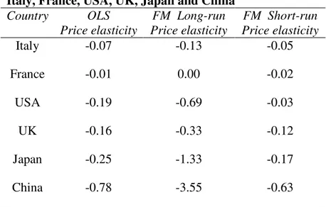
The average long-run price and income elasticities are found to be approximately -1 and +1,5, respectively; the run price elasticities present an average of -0,21 and the average short-run income elasticity is 0,41. Thus, exports do react to both the trade partners’ income and to relative prices. According to the results of the estimation, exports seem to be much more responsive to changes in relative prices in the long-run than in the short-run. In particular, among the 53 countries investigated, there are Italy, France, Japan, USA, UK and China (5 of the 6 countries analyzed in the present research) and the reported FM export price elasticities are:
Table 2.1 Export price elasticities using FM-OLS for Italy, France, USA, UK, Japan and China
Country OLS Price elasticity FM Long-run Price elasticity FM Short-run Price elasticity Italy -0.07 -0.13 -0.05 France -0.01 0.00 -0.02 USA -0.19 -0.69 -0.03 UK -0.16 -0.33 -0.12 Japan -0.25 -1.33 -0.17 China -0.78 -3.55 -0.63
Table 2.1 Export price elasticities using FM-OLS. Source: Senhadji and Montenegro (1999).
Asian countries show significantly higher price elasticities than both industrial and developing countries. In addition, according to the authors’ results, Asian countries benefit from higher income elasticities than the rest of the developing world, corroborating the general view that trade has been a powerful engine of growth for these economies.
28
3.3DOLSapproach
The Ordinary Least Squares (OLS) method provides estimates of the regression slopes that are consistent and converge at rate T where T is the sample size. When there is correlation between the regression error and the regressors, i.e. endogeneity, OLS estimates have an asymptotic bias which makes inference difficult. In order to overcome this bias, several methods have been proposed, and, besides the FM approach, one of these is the Dynamic OLS model (DOLS). The dynamic OLS (DOLS) approach proposed by Stock and Watson (1993) augments the original regression with lags of the first differences of the regressors. If the lag structure is chosen in a suitable way, the asymptotic bias is removed but the choice of lag remains an important practical issue and often researches do not have a practical guidance on how to choose them.
In the equation19:
Yt = α + Xt + εt (2.6)
is the cointegration coefficient and it is the result of an OLS regression.
If Xt and Yt are cointegrated, the OLS estimator in the regression of the cointegration
coefficient in (2.6) will be inconsistent. Generally, the OLS estimator can lead to problems and to wrong results. For this reason, econometricians have developed alternative estimators able to measure the cointegration coefficient. One of these estimators is exactly the DOLS. The DOLS estimator is based on a modified version of equation (2.6) that includes past, present and future values of Xt:
Yt = β0 + Xt + ∑ ∆Xt-j + ut (2.7)
Therefore in equation (2.7), the regressors are: Xt, ∆Xt+p, …∆Xt-p. The DOLS estimator of
is the OLS estimator of in equation (2.6).
If Xtand Ytare cointegrated and the sample is numerous enough, then the DOLS estimator is
efficient. Furthermore, since Xt and Yt , being cointegrated, have a common stochastic trend, the
DOLS estimator remains consistent even if Xt is endogenous.
The Dynamic OLS (DOLS) approach is used by Aziz and Li (2007) to estimate the export and import equations for China using quarterly data from 1995:Q1−2006:Q4. DOLS is chosen
19
29
because of its small sample property: indeed, Monte Carlo experiments show that with finite sample, DOLS performs well.
According to the authors, using aggregate data, export elasticity to foreign demand is +3.8, and to relative price is −1.6. These estimates are within the range of other studies (Goldstein and Khan, 1985) and satisfy the Marshall-Lerner condition. In the discussion of the results, the authors argue that great cautious is needed when using trade elasticities to estimate the response of the Chinese economy to price and demand shocks. Trade elasticities used in existing studies on such subjects vary widely and such variation reflects not only data and methodological issues involved in estimating elasticities for all countries, including developed countries, but also a continuous structural shift in how production is organized in China. China is shifting away from stereotypical processing trade that involves mostly assembling imported parts and components to domestically sourcing larger portions of the production chain (Aziz and Li, 2007). In conclusion, the fast changing structure of China’s trade also raises questions about how much one can rely on these estimates, especially the interaction between exchange rate and trade composition changes. Any analysis that does not take into account these factors, continuing to be influenced by China’s past trade structure could lead to erroneous outcomes.
The DOLS procedure has been also adopted by Caporale and Chui (1999) to estimate the long-run income and price elasticities of trade for 21 countries, using annual data over the period 1960-1992, in a cointegration framework. According to the authors, faster growing economies have high income elasticities of demand for their exports but lower import elasticities. For what concerns in particular Italy, Germany, France, Japan, USA and UK the export elasticities estimates are:
Table 2.2 Price and income export elasticities using DOLS for Italy, France, USA, UK, Japan and Germany.
Country DOLS Price elasticity DOLS Income elasticity Italy -0.93 2.21 France -0.08 2.13 USA -0.63 1.40 UK -0.19 1.29 Japan -1.70 2.91

![[SPS seminar. Clinical psychology and disability] - Some reflections on the concept of family.](data:image/gif;base64,R0lGODlhAQABAIAAAP///wAAACH5BAEAAAAALAAAAAABAAEAAAICRAEAOw==)