Characterization of real aquifers using hydrogeophysical measurements. An application to the chambo aquifer (Ecuador)

(1)

UNIVERSITÀ DELLA CALABRIA

Dipartimento in INGEGNERIA PER L’AMBIENTE, IL TERRITORIO E INGEGNERIA CHIMICA

(sede amministrativa del Corso di Dottorato)

Scuola di Dottorato in Scienze Ingegneristiche “PITAGORA”

Dottorato di Ricerca in

INGEGNERIA IDRAULICA PER L’AMBIENTE E IL

TERRITORIO

Con il contributo di:

SECRETARIA NACIONAL DE EDUCACIÓN SUPERIOR, CIENCIA, TECNOLOGIA E INNOVACION (SENESCYT – ECUADOR)

CICLO XXVII

CHARACTERIZATION OF REAL AQUIFERS USING

HYDROGEOPHYSICAL MEASUREMENTS. AN APPLICATION TO THE CHAMBO AQUIFER (ECUADOR).

Settore Scientifico Disciplinare ICAR/02

Coordinatore: Ch.mo Prof. FRANCESCO MACCHIONE

Supervisore: Ing. Prof. SALVATORE STRAFACE

(2)

El amor y la ternura de tu presencia lo es todo para mi, haces que cada día quiera ser siempre mejor, con mucho amor.

Para ti

(3)

INTRODUCTION

Groundwater is the most important water supply for drinkable and irrigational use. The strong interconnection between hydrologic, soil and atmospheric systems allows the circulation of different pollutants. Pollution strongly reduces useful water supply which should be able to satisfy community needs. The combination of the classical disciplines of hydrogeology with the technological development of geophysics, allows rapid acquisition and interpretation of high-resolution information, using noninvasive, nondestructive and low cost techniques. The purpose of this thesis is the adoption of new approaches to improve aquifer characterization and monitoring by means of hydrogeophysical methodologies.

Several experimental tests have been performed both at a laboratory and field scale: we started from the study of the hydrodispersive parameters of the soil through the execution of tracer tests carried out within flow cells, and we continued with the monitoring of the hydrocarbons concentration performed with Ground Penetrating Radar (GPR) techniques in a sandbox, to finish with Self Potential (SP) measurement in the Experimental well field of University of Calabria.

The acquired data, have been interpreted by means of an iterative inverse procedure based on a finite element model simulating multiphysical problems. Depending on the case, you can solve coupled equations systems describing the experiment under examination, i.e. the transport and groundwater flow phenomena, or the two-phase flow for immiscible fluids, or the Poisson-Darcy model for the evaluation of the electrical potential generated by the water flowing into a porous medium.

The Know-how acquired studying laboratory and experimental field tests, has been than applied in a real problem, regarding the water supply of the Chambo Aquifer in the Province of Chimborazo – Ecuador. The main goal of the study was the determination of the aquifer recharge over time, to demonstrate that that is the groundwater system is not fossil. The first step of the analysis, was the reconstruction of the basin domain through the interpretation and interpolation of different data types. A geographic

(4)

information system (GIS) of the area was performed through the processing of satellite images (ASTER) together with the information provided by the Ecuadorian Confederation of Agricultural Services (CESA), allowing the reconstruction of the Chambo basin, which has an approximate area of 3589.55 km2. The superficial hydrological system of the basin consists of thirty-three tributaries that come from different directions and fed the Chambo River. The main tributaries are the Cebadas River, which comes from the southern boundary of the basin, and the Guano River coming from the north. The Alao and Guamote Rivers are major tributaries coming from the West and East, respectively. The superficial water balance was calculated in the ArcGIS environment, using average temperature and rainfall data for the entire year. These data come from the Meteorological Annuary of the National Institute of Meteorology and Hydrology (INAMHI). The aquifer boundaries were defined through the information derived from the geological map of the basin. This process allowed to locate the aquifer within the Riobamba Formation, which includes incoherent pyroclastic rocks , gravel and sand. The demarcation of the boundaries allowed the identification of a potential groundwater recharge coming from the Chimborazo Volcano. The reconstruction of the model surface was obtained from Digital Terrain Model (DTM)data , while the bottom was obtained from the ordinary kriging of the information collected during a Vertical Electrical Sounding (VES) campaign. The spatial distribution of the hydraulic conductivity was derived from the ordinary kriging of puctual valuesobtained from the interpretation of the several pumping tests conducted in the aquifer area. The hydrological forcings included in the model are: a) the principal rivers: Guano, Chibunga and Chambo; b) the complex system of wells with a total pumping rate of 600 l/s, this withdrawal guarantees the water supply of drinkable water for the cities of Riobamba and Guano; c) and the net-infiltration determined by the superficial water balance. The boundary conditions adopted in the model are: a) Neuman boundary conditions, on the side from which a water flowrate it’s expected from the Chimborazo volcano, whose estimation is the goal of the study; b) a Dirichlet boundary condition applied to sides influenced by the rivers; c) and a no-flow boundary conditions in the other contours. The water volume of lateral recharge was obtained from the model calibration , in which hydraulic head data supplied by springs and ponds (points where the watertable outlooks on the ground surface ) and the ones measured in the piezometers have been adopted to condition the inversion process. Once the mathematical model has been set up, the inversion of twelve different

(5)

scenarios representing the monthly groundwater variation during a year, was carried out. The results show the existence of a water flow coming from the north-western part of the model, representing the contact point with the southern slope of the Chimborazo volcano, with an approximate monthly value of 2 m3/s. The hydro-geological model was built and executed with the MODFLOW code, while the inverse procedure was conducted by the PEST software. This approach, gave back a very good fitting between the calculated and observed hydraulic heads, demonstrating that the Chimborazo Volcano contributes with a 63% of the volume to the groundwater recharge, compared with the 37% coming from other hydrological forcings, moreover, the rivers receive the largest volume of water leaving the aquifer with 82% of the total outgoing volume . This study demonstrates that the Chambo aquifer is not fossil , i.e. is fed by a lateral recharge of approximately 2 m3_{/s, which come from the glaciers of Chimborazo} Volcano. The results of this study, together with the ones coming from the 14C analyses, suggest that the reserve of ancestral ice of the Chimborazo glacier are dissolving, highlighting the influence of the climate change in Ecuador and, hence, in the world.

(6)

INTRODUZIONE

Le acque di falda costituiscono la più preziosa riserva idrica ad uso potabile ed irriguo. La forte interconnessione esistente tra sistemi idrici sotterranei e superficiali e fra questi e il suolo e l'aria, favorisce la messa in circolo di inquinanti di svariata natura e composizione. Di conseguenza, l'inquinamento riduce notevolmente la possibilità di utilizzazione di risorse idriche che dovrebbe sarebbero quantitativamente in grado di soddisfare le esigenze della comunità. L’unione tra le discipline classiche dell’idrogeologia ed i recenti sviluppi tecnologici della geofisica, consente l’acquisizione e l’interpretazione rapida di informazioni ad alta risoluzione sfruttando tecniche non invasive e non distruttive con minori oneri economici rispetto alle indagini dirette. Il lavoro di tesi si inserisce in tale contesto, con l'obiettivo di sviluppare e adottare nuove metodologie idrogeofisiche, per migliorare la caratterizzazione ed il monitoraggio degli acquiferi.

A tale scopo sono stati eseguiti diversi test sperimentali a scala di laboratorio e di campo: partendo dallo studio dei parametri idrodispersivi del suolo mediante l'esecuzione di prove di tracciamento effettuate su celle di flusso, si è passati ad esperimenti di monitoraggio della concentrazione di idrocarburi con l’uso del Ground Penetrating Radar (GPR) in un sandbox, per giungere al monitoraggio della falda del campo Prove dell’Università della Calabria sito a Montalto Uffugo, attraverso l’interpretazione di misure di potenziale spontaneo (SP).

I dati acquisiti, sono stati invertiti attraverso una procedura iterativa basata su un modello agli elementi finiti che consente l’implementazione di problemi multifisici. A seconda dei casi, è possibile accoppiare e risolvere le equazioni che descrivono i fenomeni che avvengono negli esperimenti, come il flusso ed il trasporto delle acque sotterranee, il flusso bifase per fluidi immiscibili o ancora il potenziale elettrico generato dall'acqua che scorre in un mezzo poroso (modello Darcy-Poisson)

Le metodologie studiate in laboratorio e su campo sperimentale, sono state quindi applicate per lo studio di un problema reale inerente alla falda acquifera del Chambo nella provincia di Chimborazo – Ecuador. Il duplice obiettivo dello studio è stato quello di determinare la ricarica idrica della falda nel tempo e dimostrare che quest’ultima non

(7)

è fossile. Il primo passo è stato la ricostruzione del dominio del bacino attraverso l'interpretazione e l'interpolazione di dati di varia natura. Attraverso l'elaborazione, in ambiente GIS, di immagini satellitari di tipo ASTER e delle informazioni fornite dal Central Ecuatoriana de Servicios Agricolas CESA, è stata effettuata la ricostruzione del bacino del fiume Chambo e la determinazione della sua superficie, che è risultata pari a circa 3589.55 Km2. Il sistema idrologico superficiale del bacino è costituito da trentatre affluenti che provenendo da direzioni differenti alimentano il fiume Chambo. I principali affluenti sono il rio Cebadas, che proviene dal confine meridionale del bacino, ed il rio Guano che proviene da Nord. I fiumi Guamote e Alao sono invece i principali affluenti che provengono rispettivamente da Ovest ed Est. Inserendo i dati di temperatura e pioggia, provenienti dall'annuario metereologico dell'Istituto di Metereologia e Idrologia (INAMHI), nella ricostruzione del bacino in ambiente GIS, è stato possibile determinare il bilancio idrico superficiale, valutato mensilmente nel corso di un anno. La falda acquifera presente nel bacino, è stata invece delimitata utilizzando le informazioni provenienti dalla carta geologica del bacino, che ha consentito la localizzazione del bacino sotterraneo all'interno della formazione detta Riobamba, la quale comprende per lo più rocce piroclastiche incoerenti, ghiaia e sabbia. La delimitazione dei confini della falda, ha quindi consentito di individuare il dominio di modellazione per la stima di un eventuale ricarica idrica sotterranea proveniente dal versante del vulcano Chimoborazo. La ricostruzione della parte superficiale del modello del flusso idrico sotterraneo è stata ottenuta dai dati provenienti dal DTM, mentre il bottom attraverso l'ordinary kriging delle informazioni ricavate da una campagna di Sondaggi Elettrici Verticali (SEV). La distribuzione spaziale della conducibilità idraulica è stata derivata da un ordinary kriging dei valori puntuali di K, ricavati dall'interpretazione di diverse prove di emungimento realizzate nel bacino. Le forzanti idrologiche inserite nel modello sono rappresentate a) dai fiumi principali: il Guano, il Chibunga ed il Chambo; b) dal complesso sistema di pozzi presenti nell'area che, per garantire l'approvvigionamento idrico di acqua potabile alle città di Guano e Riobamba, emungono complessivamente una portata di 600 l/s; c) l'infiltrazione netta determinata attraverso il bilancio idrico superficiale. Per quanto riguarda le condizioni al contorno adottate nel modello, sono state adottate, una condizione alla Neuman sul confine da cui dovrebbe entrare un flusso idrico proveniente dal vulcano Chimborazo, la cui stima è l'obbiettivo dello studio, una condizione alla Dirichlet sui contorni interessati dalla presenza dei fiumi ed una condizione di flusso nullo sui restanti contorni. La

(8)

calibrazione del modello e quindi la stima della ricarica idrica laterale, è stata ottenuta utilizzando i dati di carico idraulico forniti da sorgenti, e stagni (punti in cui la falda acquifera si affaccia sulla superficie del suolo) e quelli misurati nei piezometri. Una volta aver definito l'impostazione del modello matematico, è stata effettuata l'inversione di dodici scenari mensili differenti, che hanno tutti mostrato l'esistenza di un flusso d'acqua di circa 2 m3/s, proveniente dalla zona Nord-occidentale del modello che rappresenta il punto di contatto con il versante Sud del vulcano Chimborazo. Il modello idrogeologico è stato implementato ed eseguito con il codice MODFLOW, mentre la procedura di inversione è stata condotta attraverso il software PEST. Il loro uso congiunto sui dodici modelli implementati, ha restituito un ottimo fitting tra i carichi idraulici calcolati e quelli osservati. Si è dimostrato quindi che il Chimborazo contribuisce al 63% del volume di ricarica idrica sotterranea contro il 37% proveniente dalle altre forzanti idrologiche, e che il maggior volume di acqua esce dalla falda attraverso i fiumi con 82% in uscita.

Questo studio dimostra che l'acquifero del Chambo non è di natura fossile ma viene alimentato da una ricarica laterale di circa 2 m3/s proveniente dal ghiacciaio del vulcano Chimborazo. I risultati di questo studio, insieme a quelli ottenuti da un analisi effettuata con il 14_{C, suggeriscono che le riserve di ghiaccio ancestrale sul vulcano si stanno} sciogliendo, mettendo in evidenza il possibile impatto dei cambiamenti climatici in Ecuador e quindi nel mondo.

(9)

List of Figures

Figure 1. 1: (modified from Rubin and Hubbard, 2005) a schematic diagram of field geophysical length scale resolution and study objective scale. ... 22 Figure 1. 2: Flux diagram showing the forward and inverse processes. On the left an example of calculated and observed data and on the right created and inverted models. ... 24 Figure 1. 3 : Electrical resistivity and conductivity of Earth materials (modified from Palacky, 1988). 25 Figure 1. 4: Wave nature of electromagnetic fields. A moving charge of current creates a magnetic field B which induces an electric field E which in turn causes electric charges to move and so forth (modified after Annan, 2005). ... 28 Figure 1. 5: Measurement distribution of a surface resistivity arrangement that built the resistivity pseudosection. ... 32 Figure 1. 6: Left, Time domain IP waveform showing the primary voltage Vp, the secondary voltage Vs, and the integration window. On the right, frequency domain IP waveform showing IP response defined as a phase lag in the received waveform (Modified after Zonge et al., 2006). ... 33 Figure 1. 7: On the left, transmitter and receiver coil and electromagnetic waves distribution in the Earth’s interior. On the right, transient decay curves for a loop-‐loop system at different separation distances over a uniform halfspace (0.1 S/m). The transient time of the sign reversal increases with increasing Tx-‐Rx separation from 10, 30, to 60, to 100 m. Dashed line negative voltage, solid line positive voltage (from Everett and Meju, 2005). ... 36 Figure 1. 8: Geometry of a typical loop-‐loop system. Coils can operate either in a vertical or horizontal configuration, achieving different investigation depth and lateral resolution. ... 38 Figure 1. 9: On the left NMR instrument application. On the right detail of the hydrogen proton

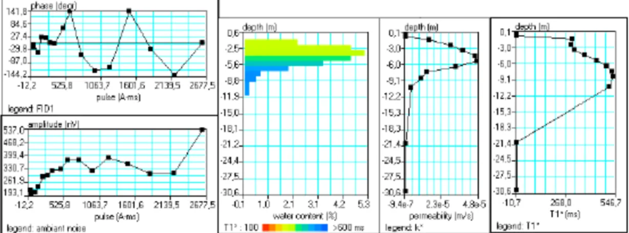
deflection due to the induced current at the Larmor frequency (from Yaramanci et al., 2005). ... 42 Figure 1. 10: Input and output signals of NMR (from Yaramanci et al., 2005). ... 42 Figure 1. 11: Typical data (left) and inversion models (right) of an NMR sounding on La Soutte

(Behaegel 2006), where water content and permeability have been estimated. ... 43 Figure 1. 12: Geometric relationships between surface, reflected, direct and refracted (headwave) waves (From Pelton, 2006). ... 46 Figure 1. 13: Archie type petrophysical relationship. F is formation factor and is porosity extracted from laboratory studies. C is conductivity and Cf is the fluid conductivity. Linial regression is derived and subsequently applied at the same locality, when only one of the two variables is known (from Purvance and Andricevic, 2000). ... 50

(14)

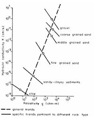
Figure 1. 14: Relationships between hydraulic conductivity and resistivity for different rock types

(direct correlation) and within a specific rock types (inverse correlation) (from Mázac et al., 1990). . 52

Figure 1. 15: Left, resistivity versus salinity concentration (CNaCl) for samples with different clay content samples showing two different dominant resistivity process. Right, the relationship between porosity and clay content. Total porosity decreases due to increasing clay content up to a critical point, where after it starts to increase, and conversely effective porosity decreases (modified form Shevnin, 2006). ... 53

Figure 1. 16: Compilation of measurements of specific porous surface area Spor and imaginary electric component σ’’ from different materials and studies, showing a consistent relationship (from Slater, 2006). ... 54

Figure 2. 1: Experimental setup for a gas dispersion and b solute dispersion measurements ... 63

Figure 2. 2: Best-‐fit curves for the single and the dual phase model (Granite) ... 65

Figure 2. 3: Best-‐fit curves for the single and the dual phase model (Gravel) ... 65

Figure 2. 4: Best-‐fit curves for the single and the dual phase model (Leca®_{)
...
66}

Figure 2. 5: α calculated (cm) [Pugliese et al., 2013a,b] vs α calculated (cm) [Mendoza] for the Granite ... 68

Figure 2. 6: α calculated (cm) [Pugliese et al., 2013a,b] vs α calculated (cm) [Mendoza] for the Gravel ... 68

Figure 2. 7: α calculated (cm) [Pugliese et al., 2013a,b] vs α calculated (cm) [Mendoza] for the Leca® ... 68

Figure 2. 8: 2D Sandbox in plexiglass ... 76

Figure 2. 9: Front side of the 2D Sandbox whit twenty-‐one extraction holes of 16 mm ... 77

Figure 2. 10: Hydraulic loading system: (a) collection tank; (b) loading tank. ... 77

Figure 2. 11: Hydrocarbon injection by means of a peristaltic pump ... 78

Figure 2. 12: a) SIR 3000 GPR used for data acquisition. b) Antenna GPR, 2000Hz. 1-‐wheel equipped with recorder; Mini 2-‐replaceable plate; 3-‐Fiber optic cable; 4-‐ Deadman switch (safety switch); 5-‐ removable knob; 6-‐Marker to switch. ... 78

Figure 2. 13: Grid of acquisition located behind the Sandbox. ... 79

Figure 2. 14: Syringe sampler applied to the front face of the SandBox. a) pierced junction plate applied with perspex liquid (left) and sections of the piece (right). b) Sampling syringe (left) and its components (right). ... 80

Figure 2. 15: a) Sandbox samplers configuration and b) Sampling operations ... 80

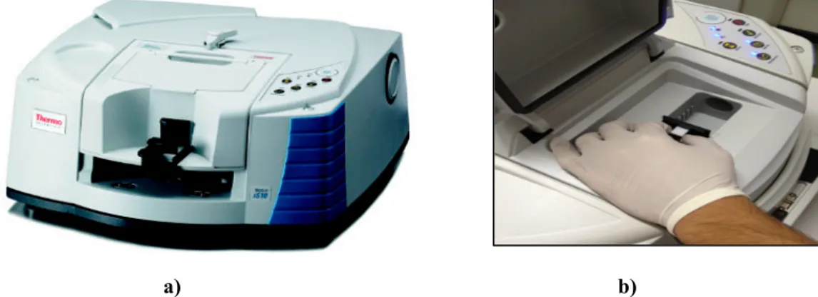
Figure 2. 16: a) Infrared Spectrophotometry Thermo FT-‐IR Nicolet iS10 b) LNPL samples analysis ... 81

Figure 2. 17: Typical curves of TPHs derived from the infrared spectrophotometer for an absorbance range of 2800 -‐ 3000 cm-‐1_{...
81}

Figure 2. 18: Permittivity map during water saturated conditions. ... 82

(15)

Figure 2. 20: Interpolated contrast permittivity map realized by the differences recorded between the

water saturated conditions map and the scenarios acquired the sixth day from the diesel injection. ... 83

Figure 2. 21: Contrast map expressed in saturation degree Sw percentage. ... 83

Figure 2. 22: a) Experimental well field of University of Calabria, b) 1 office 2 laboratory hydraulic models 3 warehouse 4 laboratory analysis of water and 5 field tests. ... 85

Figure 2. 23: A schematic illustration of the layout of the well field of Montalto Uffugo Scalo and our conceptual model of its geology (Straface et al., 2007) ... 86

Figure 2. 24: Scheme of arrangement of the SP monitoring points and wells ... 87

Figure 2. 25: Contact gauge KL 010 ... 88

Figure 2. 26: Mini-‐Diver ... 88

Figure 2. 27: Baro-‐Diver ... 89

Figure 2. 28: Nonpolarizing Pb/PbCl2 (Petiau) electrodes ... 90

Figure 2. 29: Keithley 2701 multichannel voltmeter ... 90

Figure 2. 30: Multimeter PCE-‐DM 22 ... 91

Figure 2. 31: Scheme adopted for the hydraulic heads calculation ... 91

Figure 2. 32: Hydraulic head variations in wells 2, 4, 6, 8, 10 ... 92

Figure 2. 33: a) Bentonite base b) Electrode with bentonite ... 93

Figure 2. 34: Self-‐Potential measurement with Multimeter PCE-‐DM 22 ... 93

Figure 2. 35: SP signals acquired in the 50 measurement points ... 99

Figure 2. 36: Trend of the temperature values in the time ... 99

Figure 2. 37: Precipitations during July, Montalto Uffugo – ARPACAL ... 99

Figure 2. 38: Time evolution maps of the hydraulic head distribution (left) and SP signals (right) .... 105

Figure 2. 39: Area with the presence of wells and metal parts ... 106

Figure 2. 40: The hydrogeological model ... 107

Figure 2. 41: Wells in the model domain ... 112

Figure 2. 42: Hydraulic head (5 wells) with respect to time ... 113

Figure 2. 43: SP signal points in the model domain ... 114

Figure 2. 44: SP signal in all the observation points ... 114

Figure 2. 45: Confrontation between SP and hydraulic head (Piezometer 6 in red, Point 2 in blue) ... 115

Figure 2. 46: Confrontation between SP smoothed (blue) and simulated (red) ... 117

Figure 3. 1: The Chambo Sub-‐basin in Ecuador ... 120

Figure 3. 2: Micro-‐basins of the Chambo Sub-‐basin (Naranjo, 2013) ... 121

Figure 3. 3: Geologic map of the Chambo Subbasin (Naranjo, 2013) ... 123

Figure 3. 4: Hydrogeological map of the Chambo River Sub-‐basin (Naranjo, 2013) ... 133

Figure 3. 5: Geological cut in the Riobamba area (Naranjo, 2013) ... 135

Figure 3. 6: Map with the locations of all the geological correlations performed at the Chambo Aquifer in Riobamba (Naranjo, 2013). ... 136

(16)

Figure 3. 8: Correlation Wells within the Riobamba area in a NW-‐SE direction (Naranjo 2013). ... 138

Figure 3. 9: Transmissivity map of the Chambo aquifer in Riobamba (Naranjo, 2013). ... 140

Figure 3. 10: Geological section of the Chambo aquifer at Llío San Pablo, derived from the geoelectrical investigation, (Naranjo, 2013). ... 141

Figure 3. 11: Location map of the Llío – San Pablo aquifer (Naranjo, 2013). ... 142

Figure 3. 12: Hydrogeological interpretation of the Chambo aquifer at Llío – San Pablo. (Naranjo, 2013). ... 143

Figure 3. 13: Boreholes correlation in the Yaruquíes’ aquifer in a (W-‐E) (Naranjo, 2013) ... 144

Figure 3. 14: Hydrogeological map of the Chambo aquifer at Punín (Naranjo, 2013). ... 146

Figure 3. 15: Geological section of the Guano area (Naranjo, 2013). ... 147

Figure 3. 16: Micro-‐basins at the Chambo River sub-‐basin. ... 149

Figure 3. 17: Elevation map of the Chambo River sub-‐basin (Naranjo, 2013). ... 153

Figure 3. 18: Elevation map from the Chambo river sub-‐basin (Naranjo, 2013). ... 154

Figure 3. 19: Curved distribution of the slopes at the Chambo river sub basin (Naranjo, 2013). ... 155

Figure 3. 20: Topographic cut through the Chambo, Cebadas and Altillo rivers (Naranjo, 2013). ... 155

Figure 3. 21: Chambo river basin boundaries. ... 158

Figure 3. 22: Rainfall at one point in the Chambo sub-‐basin ... 160

Figure 3. 23: Rainfall in Chambo the sub-‐basin for the entire year. ... 160

Figure 3. 24: a) Evapotranspiration at one point in the subbasin of the Chambo River year round b) Evapotranspiration in the Chambo sub-‐basin during January. ... 161

Figure 3. 25: a) Runoff at one point in the Chambo sub-‐basin during one year b) runoff at the Chambo sub-‐basin and the change of the values between January and March. ... 161

Figure 3. 26: a) Infiltration at one point in the Chambo sub-‐basin over the course of a year b) Infiltration at the Chambo sub-‐basin and the change of values between February and March. ... 162

Figure 3. 27: Infiltration in the Chambo aquifer during the whole year. ... 162

Figure 3. 28: Chambo river basin geology. ... 170

Figure 3. 29: a) Aquifer geological boundaries b) Aquifer modeling boundaries ... 171

Figure 3. 30: a) DTM surface of the aquifer b) Kriging of the aquifer’s bottom. ... 171

Figure 3. 31: Distribution of Hydraulic Conductivity K (m/s) ... 172

Figure 3. 32: a) Rives and wells present at the aquifer b) infiltration (mm/month) ... 172

Figure 3. 33: Observation points ... 174

Figure 3. 34: Estimated flow rate variations coming from the Chimborazo. ... 174

Figure 3. 35: Confrontation between observed and calculated hydraulic head ... 176

(17)

List of Tables

Table 1. 1: Geophysical Methods, Obtained properties and Hydrogeological objectives ... 21

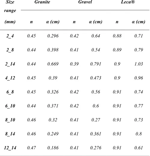
Table 2. 1: Values of effective porosity (nc), dispersivity (α), tortuosity (λ) and linear regression coefficient for the single phase model (SP) and the double phase model (DP) ... 67

Table 2. 2: Values of Total porosity (n) and dispersivity (α) for Granite, Gravel and Leca Pugliese et al. 2013a and Pugliese et al. 2013b. ... 67

Table 3. 1: Water levels monitoring at the Riobamba aquifer (Naranjo, 2013). ... 137

Table 3. 2: Hydrogeological properties of the the Riobamba area ... 139

Table 3. 3: Water level measurements in the Chambo River at Yaruquíes. ... 145

Table 3. 4: Sub-‐basin and micro basin dimension from the Chambo River (Naranjo, 2013). ... 150

Table 3. 5: Form, drainage densities, and sinuosity coefficients from the sub-‐basin and micro-‐basins of the Chambo River (Naranjo, 2013). ... 151

Table 3. 6: Water Balance at the Chambo basin at a point (mm/month) ... 159

(18)

CHAPTER 1

1.1 HYDROGEOPHYSICS

1.1.1 New frontiers in the characterization of Porous Media

parameters

The aim of this chapter is to present an overview of the geophysical methodologies for the measurement, characterization and modeling of porous media parameters. Special emphasis is given to electric and electromagnetic measurements which strongly depend on soil characteristics and water content, but other geophysical techniques which are very promising for hydrologic studies are also taken into consideration. The principles and field applications of these methodologies are briefly discussed, including main concerns and limitations. In last few years, geophysics techniques have driven the attention of many researchers interested to the investigation of near surface hydrology problems. These techniques are based on easy geophysical measurements which can be used to monitor fundamental hydrologic processes (Rubin and Hubbard 2005).

Conventional hydrologic technologies, normally applied to characterize the shallow subsurface, typically involve piezometric measurements in carved wells. Such measurements are usually sparsely distributed and do not consent, in many cases, to take into an appropriately consideration the hydrologic heterogeneity of the sites, specially when the area under investigation is very large with respect to the size of typical homogeneous region of the investigated sites. In these cases geophysics

(19)

measurements can be used to acquire complementary data to better define the problem under investigation. In fact these techniques are not invasive and can be taken at a much big density with respect to piezometer measurements. For this reason they consent to obtain more precise bidimensional and tridimensional picture of the investigate sites. The main categories of hydrologic problems that can be solved by geophysics techniques are:

Hydrological Mapping.

Under this denominations are be classified actions such as: the definition of aquifers geometry; the determination of water table level, basement and boundaries; the fresh and salt water interfaces, contaminant plumes, fracture zones etc. (Goldman, 2003; Arango 2005; Mcpheeet al. 2006). In mapping studies, the integration of sparse borehole measurements with continuous geophysics data is usually used in order to overcome the problems arising from the heterogeneity of the subsoil. An excellent review of such a strategic approach to obtain reliable volumetric hydraulic permeability is due to Sanchez-Vila et. al. (2006)

Hydrologic parameter estimation

That is to say the estimation of the water content, water quality and effective-volumetric parameter. In these case geophysical information are calibrated with directly measured hydrological data both at field scale or at laboratory level, in such a way that they can provide a more complete estimation of hydrological parameters (Ferrè et. al. 2005; Tullen et.al. 2006). Usually aquifer flow and transport properties are derived by numerical models where geophysical data are also inserted. For instance, the Hydraulic conductivity K and porosity φ defined as:

µ ρ gk

K w

= ϕ =Vp V_t

Where

ρ

w is the density of the pore fluid g is the gravitational acceleration µ the fluid

dynamic viscosity and K is the hydraulic permeability, Vp and Vt are the pore volumes and total volume respectively Now, it is assumed that the parameters inserted into the above equations can be derived from measurable geophysical properties such us electrical resistivity, dielectric constant, acoustic porosity.

(20)

Hydrologic processes monitoring of subtle geophysical property changes, caused by

natural or forced systems: common examples are the changes of water content and water quality (Slater et al., 1997; Singha and Gorelick, 2005; Tezkan et al., 2005). Dynamic transformations in flow and transport processes are monitored by time-lapse measurements of geophysical properties at the same location. Generally the, conventional Hydrological measurement suffer by the lack of a total survey repeatability at different time at a given sounding location, and these problems may introduce uncertainty into the results while looking for quantitative rates of change. When using geophysical measurement, which consent a more precise sounding location, the repeatability uncertainty of time-lapse models decreases, at benefit of the data inversion procedures, especially if constraining unchanging targets are retrieved on all the models. It must be considered that in shallow surface studies identical positioning plays a major role in performing quantitative investigations. The following table shows the main application of geophysics methodologies to hydrologic problems in different scale application.

Geophysical Methods Obtained properties Hydrogeological objectives

Airborne

Satellite

Remote sensing

Aeromagnetic Electromagnetic

Gamma radiation, Thermal radiation, Electromagnetic

Reflectivity, gravity Electrical resistivity

Bedrock mapping, faults, hydrothermalism, aquifer characterization and regional water quality

Surface

Seismic Refraction P-ware velocity Bedrock mapping, water table, faults Seismic Reflection P-ware reflectivity and velocity Stratigraphy, bedrock and faults

delineation Electromagnetic (TDEM,

FDEM, CSEM, AMT)

IP

Electrical resistivity Electrical resistivity

Complex electrical resistivity

Aquifer zonation, water table, bedrock, fresh and salt-water interfaces and plume boundaries, estimation of hydraulic conductivity, estimation and monitoring of water content and quality

(21)

GPR Dielectric constant values and dielectric contrast

Stratigraphy, water table, water content estimation and monitoring

NMR Water content, mobile water content, pore

structure Cross hole Electrical Resistivity DC GPR Electrical resistivity Dielectric constant

Aquifer zonation, estimation monitoring of water content and water quality

Seismic P-wave velocity Lithology, estimation and fracture zone detection

Well bore Geophysical well logs Many properties such as electrical resistivity, seismic velocity, and gamma ray

Lithology water content, water quality, fracture imaging

Table 1. 1: Geophysical Methods, Obtained properties and Hydrogeological objectives

It must be also considered that the strong improvement in geophysical techniques, over the last decade, is surely linked to the exponential increase in the number and diversity of available advanced instruments, adapted to different study scales. The study scales range from satellite, remote sensing and airborne, to surface and cross-hole, and, at a more detailed scale, well logs and laboratory measurements. Satellite, remote sensing and airborne geophysics work at regional scales, providing data which can be used to draw conclusions about the regional subsurface architecture. It could also be used to identify areas of interest for carrying out more detailed ground based surveys. At the other extreme, borehole geophysics provides continuous profiling or point measurements at discrete depths, and can be related to the physical and chemical properties of the surrounding wall rock, the fluid saturation of the pore spaces in the formations, the fluid in the borehole, the well casing, or any combination of these factors.

1.1.2 Work scale

In the following figure 1.1 (modified from Rubin and Hubbard, 2005) a schematic diagram of field geophysical length scale resolution and study objective scale, is reported.

(22)

Figure 1. 1: (modified from Rubin and Hubbard, 2005) a schematic diagram of field geophysical length scale resolution and study objective scale.

Before performing any geophysical investigation, a good compromise between resolution and work scale needs to be chosen in order to identify the instrumentation and field survey design, required to achieve the wanted results. A combination of different geophysical techniques and equipments, each sensitive to a given property and/or field scale, could be required, in order to characterize, in the better way, the investigated system. Further, a combination of geophysical data with direct hydrogeological measurements could be used to get a better characterization of the subsurface at different resolutions and scales (Meju, 2000; Choudhury and Saha, 2004; Pedersen et al., 2005).

1.1.3 Modeling and inversion problems

Geophysical data can be used to extract either qualitative or quantitative estimates of the subsurface characteristics. The qualitative approach uses raw geophysical data and it is often used for preliminary mapping or to assess relative changes. These raw data images give generally a smooth image of the subsurface. The values of the investigated properties and the corresponding depth locations cannot be considered reliable at this

(23)

stage. Geophysical data require specific data processing and analysis for each given technique before modelling and inversion processes can be performed. Careful data analysis can provide further accuracy of the final models or constrain the specific modelling approach, such as the dimensionality inversion (Ledo et al., 2002 a; Martí et

al., 2004; Ledo, 2006). The transformation from raw data to an estimated geophysical

model is usually achieved using numerical forward modelling and inversion procedures, to provide a description of the subsurface fitting the observed data. Joint inversion of different geophysical sets (Gallardo and Meju, 2003; Bedrosian, 2006; Linde et al., 2007) is used to constrain the possible subsurface models with multiple independent data, using either a deterministic approach, or a probabilistic approach such as stochastic inversion methods (Deutsch and Journel, 1998; Rubin and Hubbard, 2005; Gómez-Hernández, 2005).

The interpretation of the experimental data obtained from geophysical measurementis normally made according to a procedure which can be defined as Modelling and Inversion. As a first step the researcher need to make a model of the subsurface structure, and calculate with a forward procedure the corresponding geophysical information. Then the calculated data are compared with the theoretical one, and the model is gradually changed in order to minimize the deviation of the calculated data from the experimental. This second step is considered a reverse step (Tarantola, 1987). The next figure 1.2 shows schematically the procedure. Forward modelling is a typical trial and error process that computes the responses of an input model, comparing the responses with measured data, modifying the model where the data are poorly fitted and then re-computing the responses until a satisfactory fit is obtained.

The inverse problem involves an automatic iterative process that searches for the best model, progressively reducing the misfit between the measured data and synthetic data from the model with each iteration. The iterative process proceeds until either a predefined threshold misfit value is reached or until an acceptable model is obtained. Inversion strategies used aim to achieve better numerical convergence, more stable solutions, three-dimensionality inverse modelling, and to reduce the computational time (Spichak and Popova, 2000; Zyserman and Santos, 2000; Haber et al., 2004; Siripunvaraporn et al., 2004; Avdeev, 2005; Haber, 2005; Siripunvaraporn et al., 2005 a).

(24)

Figure 1. 2: Flux diagram showing the forward and inverse processes. On the left an example of calculated and observed data and on the right created and inverted models.

The model resulting from the above described process provides an image that has to be considered an approximation of the real physical situation. First of all geophysical data are subject to measurement errors and the beginning trial model generally contains semplifications of the physical reality. Cure must be taken do not overfit data, introducing artifacts into the models. Moreover, numerical processes and coarse discretization tend to provide regionally smooth models.

Finally, a study of the sensitivity of the model is required to provide confidence in the subsurface image. It is also desirable for the estimated model to be in accord with any available previous investigation of similar problems (Binley and Kemma, 2005).

1.1.3 Base Concepts of Electrical and Electromagnetic Geophysical

Techniques

General tools

Most part of the following discussion has strongly suggested the excellent scientifical contributes of Pellerin 2002, Guerin (2005), Hubbard and Rubin (2005), Aukenet.al (2006). Electrical (E) and electromagnetic (EM) methods are the most commonly used in geophysical approaches to determine hydrogeological parameters and processes.

(25)

E&EM are particularly suitable for hydrological studies in the vadose and saturated zones, since the electrical properties of subsurface materials are highly dependent on lithology, water saturation, biochemistry of the fluid and movement of this fluid. Figure 1.3 presents the electrical resistivity of the different geological materials.

Figure 1. 3 : Electrical resistivity and conductivity of Earth materials (modified from Palacky, 1988).

When an electrical current naturally exists or is externally applied, the mobile charge carried within the soil starts to flow, and the differential charge distribution in the soil generates space differences of the electric potential. The base equation governing the current densities J and electric displacement D are:

E

J =σ D=εE

Electrical conductivity (σ) describes how free charges flow to form a current when an electric field is present and the electrical permittivity (ε) describes how charges are displaced in response to an electric field.

The measured geoelectrical properties of materials, under the application of oscillating field depend on the of frequency (ω) of the applied signal:

(26)

( )

ω

σ

( )

ω

σ

( )

ω

σ

= ' −i "

ε

( )

ω

=

ε

'

( )

ω

−i

ε

"

( )

ω

Conductivity and similarly permittivity can be expressed as a magnitude and a phase angle that relates the in-phase and the out-of-phase components:

( )

2

( )

2 " ' σ σ σ = + ⎟ ⎠ ⎞ ⎜ ⎝ ⎛ = − ' " tan 1 σ σ θ

where σ’, σ”, ε’ and ε” denotes the real’ and imaginary” electrical components known as ohmic conduction, faradic diffusion, dielectric polarization, and energy loss due to polarization, respectively. The above equations show that there is more than ohmic conduction contributing to what is measured as electrical conductivity, and there is more than dielectric polarization contributing to what is measured as effective permittivity or stored energy in the system. A point of divergence in the literature is found in the assumptions that are made about the relative importance of these four parameters in order to extract values from the measured data.

Complex electrical conductivity or, the inverse parameter, resistivity and complex permittivity contain the same information expressed differently and are related by the following expression:

* *

ωε σ =i

where * indicates a complex number and the complex components are related as:

( )

ω

σ

( )

ω

ωε

( )

ω

σ

= ' + "

( )

ω ω σ ω ε ω ε = ' + "

σ’ represents the ohmic conduction current (energy loss) detected by the DC resistivity and EM induction methods. This conduction is due to the pore-filling electrolyte and the surface conduction generated by the ion migration at the electrical double layer (EDL) (Purvance and Andricevic, 2000). σ” is related solely to the fluid-grain interface (Slater, 2006), related to the polarization (energy storage) term measured with induced polarization techniques.

When modelling electrical behaviour of soil materials at frequencies greater than 100 kHz it is commonly assumed that !"(!)_! =0 and 𝜎′(𝜔) = 𝜎_!" (Knight and Endres, 2006) therefore above relations can be rearranged as:

(27)

( )

ω σ ωε

( )

ω

σ = ' +DC " and

ε

( )

ω

=

ε

'

( )

ω

For low frequency measurements, 𝜎! _{𝜔 ≠ 𝜎}

!" and 𝜎! 𝜔 𝑖𝑠 considered the source of

the frequency dependence governing the electrical response, where two specific final cases can be defined:

1) When fluid conductivity dominates the electrical behaviour, that is ionic conduction Dominates, 𝜎! _{𝜔 ≫ 𝜔𝜀}!!_{(𝜔) thus the electric loss term 𝜀}!!_{(𝜔) can be neglected and}

effective resistivity can be formulated as:

( )

ω

σ

= ' ;

ε

( )

ω

=

ε

'

( )

ω

2) When energy loss dominates the electrical behaviour (fluid grain interface effects, ionic migration on the EDL), 𝜎!!_{(𝜔) 𝜔 ≫ 𝜀}!_{(𝜔), the electrical parameters can be}

written as:

( )

ω ω σ ω ε = " ;

σ

( )

ω

=

ωε

"

( )

ω

Further insights into the influence of type of electric characteristic of the system under investigation will be given in paragraph 1.4.2 of this chapter. This particular aspect of the problem represent one of the most important research topic still underdevelopment. Electric potential differences is actually measured in Electric and electromagnetic geophysical investigation. These parameters can be expressed as a function resistivity and permittivity values, which in turn can interpreted in terms of a geological model of the investigated site. The following sections present the main electric and electromagnetic methods used where resistivity or permittivity can be inferred.

1.1.4 Electromagnetic fundamentals

The principle behind electromagnetic methods (EM) is governed by Maxwell’s equations that describe the coupled set of electric and magnetic fields change with time: changing electric currents create magnetic fields that in turn induce electric fields which drive new currents (Figure 1.4). The EM techniques presented here (CSAMT, TDEM, FDEM, GPR and NMR) use a controlled artificial electromagnetic source as a primary field that induces a secondary magnetic field. However, other EM methods use the Earth’s natural electromagnetic fields as well (AMT). Natural EM waves are generated

(28)

by thunderstorm activity in the frequency range of interest to hydrogeophysical studies 1Hz to 1 MHz. Combining the laws of Ohm, Ampere, and Faraday and the constitutive relationships results in a wave equation, which relates electromagnetic responses to rock physics in order to quantify material properties (Everett and Meju, 2005):

Figure 1. 4: Wave nature of electromagnetic fields. A moving charge of current creates a magnetic field B which induces an electric field E which in turn causes electric charges to move and so forth (modified after Annan, 2005). s II I J t B t B B = ∇ ∂ ∂ − ∂ ∂ − ∇ 2 0 2 0 0 2 µ ε µ σ µ !" !# $ !" !# $

where B (T) is the magnetic field, µ0 (H/m) is the magnetic permeability, σ is the electrical conductivity (S/m), ε (F/m)is the electric permittivity, J (A/m2) is the source current distribution, and t (s) is time. For most hydrogeophysical applications the Earth is generally considered to be nonmagnetic and µ0 taken as the magnetic permeability of free space µ0 = 4л x 107 H/m. In highly magnetic soils or in the presence of ferrous metal objects this assumption can break down. Referring to the above equation, term I is the energy dissipation relating to the electromagnetic diffusion and term II is the energy storage describing wave propagation. The frequency of the electromagnetic waves controls the contribution of both diffusion and propagation phenomena through the Earth. The diffusion regime (ω < 100 kHz) is prevalent when term I is larger by several

(29)

orders of magnitude than the wave propagation term (II). Such condition is also called the quasi-stationary approximation. In the diffusion regime the propagation term II could be ignored and the electric permittivity plays no further role in the discussion of the AMT, TDEM, FDEM methods. In a similar manner, when the propagation term is bigger than the diffusion one (ω >1MHz), the conductivity effect is minor; in this situation the GPR is highly effective. However, problems can occur when both effects make contributions to the response of the recorded induced currents. The electromagnetic methods are sensitive to electrical resistivity and electric permittivity over a volume of ground where induced electric currents are present. Among the subsurface based geophysical methods that sense bulk electrical and effective properties of the ground, EM provides deeper penetrations depth capability and greater resolving power (Everett and Meju, 2005). EM methods are cost effective, relatively easy to operate in the field, and a variety of data processing options are available, ranging form the construction of apparent resistivity curves or pseudo-sections for a fast subsurface evaluations, to 1-D and 2D forward and inverse modelling. 3D inverse modelling is not yet fully developed although research is moving forward rapidly in this field, where new codes are being tested. However, the main concerns in all EM methods are cultural noise sources such as power lines, pipelines and DC trains among others, that screen and disturb the geophysical signal.

Electromagnetic induction methods are the most widely used and versatile geophysical methods in hydrogeology studies at different scale ranges. This diverse set of techniques and instruments available provides the possibility of conducting cross-scale investigations. Airborne electromagnetic methods are used to obtain regional survey information from watershed to basin scales and can be implemented either from a helicopter or a fixed-wing aircraft and operated in either the frequency or the time domain. Surface geophysical methods can investigate greater depths and on higher resolution (from local studies to basin scale). At a detailed resolution scale in depth there are borehole and cross-hole arrays available. Selection of the appropriate technique will be strongly influenced by study objectives, time, founds and computational facilities.

(30)

Direct Current methods (DC)

DC methods are based on the injection of a current into the ground, to measure the generated electrical field as a potential difference. The experimental configuration of the electric resistivity method consists of four electrodes. Two of them, A and B, are the current electrodes, where a current I is injected, while the other two, M and N, are the potential electrodes, where a potential difference ∆V is recorded. The potential difference measured depends on the current applied, the resistivity of the subsurface medium and the geometric factor (k) determined by the array configuration (distance between electrodes). The following expression relates these parameters to the apparent resistivity ρa: I V k a Δ = ρ

defined as the resistivity of a homogenous site to which the real site is equivalent. The apparent resistivity has to be inverted to obtain estimated resistivity versus depth. Many electrode configurations are commonly used for ground-surface surveys,

Schlumberger, Wenner, Dipole-dipole, where the electrode separations relate to the investigation depth and lateral resolution, according to the sensitivity distribution of each arrangement (Roy and Apparo, 1971; Edwards, 1977; Gabàs, 2003). There are numerous electric prospecting arrays depending on number of electrodes and its distribution on the ground. The most appropriate survey configuration (vertical electrical sounding, electrical resistivity tomography ERT or DC surface, cross-borehole) will strongly depend on the specific objectives of the project. DC resistivity surveying is one of the most widely used methods given that field survey acquisition, processing and interpretation are relatively easy to perform. DC resistivity cannot easily determine the relative importance of electrolyte and surface conductivity on the bulk-measured resistivity (Slater, 2006; Binley and Kemma, 2005; Purvance and Andricevic, 2000). However procedures for estimating hydraulic permeability and porosity have been attempted widely and will be discussed below.

Vertical electrical soundings (VES)

Vertical electrical sounding (VES) consists of a symmetric geoelectrical array that can be used to determine the electrical resistivity of the subsurface. Increasing progressively the spacing between the current electrodes AB, while keeping the potential electrodes

(31)

MN at the same position, provides a sounding curve corresponding to the apparent resistivity versus depth of at single location. The wider the electrode spacing, the deeper is the investigation depth. Although the VES method is still widely used (Choudhury and Saha, 2004), nowadays VES is regarded as an out-dated technique as there are alternative instrumentation and electrode configurations that can provide 2D or 3D images of the subsurface more time-effectively.

Electrical surface imaging (DC or ERT)

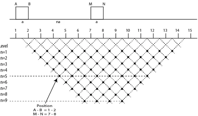
Electrical surface imaging (DC surface) called as well Electrical Resistivity Tomography (ERT), combines surface profiling with vertical soundings using a multi-electrode array to produce 2D or 3D images of the subsurface resistivity. The measurements are acquired along profiles using a large number of electrodes placed equidistantly, allowing the electrodes to be current and potential electrodes alternately. The procedure is repeated for as many combinations of source and receiver electrode positions as is defined by the survey configuration to create a full set of measurements (Figure 1.5). In new instrumentation developments continuous recording systems has been implemented that consist of fixed electrode configurations taking measurements continuously as the instrument is towed over the ground such as for example the “Ohm-mapper” system (Geometrics) or “Paces” system (Sørensen, 1996).

Measured data are presented as a pseudo-section in which the apparent resistivity is assigned to the midpoint of the four electrodes for each survey level (related to the spacing between current and potential electrodes) (Figure 1.5). The pseudo-section provides a smooth image of the ‘true’ resistivity structure with depth, so does not reproduce correctly either the electrical resistivity contrast between structures, or its exact spatial position.

(32)

Figure 1. 5: Measurement distribution of a surface resistivity arrangement that built the resistivity pseudosection.

Solving the inverse problem is necessary to obtain the estimated resistivity with depth. ERT is widely used in applications relating to hydrogeological problems (Slater et al., 2002; Mota et al., 2004; Auken et al., 2006 a; Wilson et al., 2006). Work scales may vary from2-5 m up to 50-100 m depending on the electrode spacing and the resistivity of the ground, and limited by the strength of the current injected. DC has been used mainly to map static hydrological properties, structure or hydraulic pathways as well as to monitor temporal properties associated with changes in moisture or water quality.

Induced Polarization (IP)

Induced Polarization, IP, allows the spatial distribution of the subsurface resistivity characteristics to be determined in a similar manner to the DC method. However, IP is capable of determining the geophysical signal contribution from the pore fluids and from the fluid-grain interfaces that contribute to the real and imaginary parts of the electric conductivity. Given that IP is sensitive to the processes at the fluid-grain interface (effective clay content or internal surface area), it has been used to establish petrophysical relationships with hydraulic permeability (Knight and Nur, 1987; Purvance and Andricevic, 2000; Slater, 2006).

IP measurements are made in the field using a four electrodes arrangement using non-polarizing electrodes. The measurements are based on recording the polarization and

(33)

potential difference that occurs after applying a current in either the time or the frequency domain. Time domain IP measures the decay voltage as a function of time after stopping the current injection (Figure 1.6, left). The gradual voltage decrease as a complex function of the electrical charge polarization at the fluid-grain interface and the conduction within the pore fluid (Binley and Kemma, 2005). The measurements are used to obtain an IP apparent resistivity and an apparent chargeability ma :

(

−

)

∫

( )

= 2 1 1 2 1 t t a V t dt Vp t t m

where Vp is the primary voltage and the integral measure the decay secondary voltage withtime.In the frequency-domain mode, after injecting an alternating current of characteristic angular frequency, the resistivity magnitude and the phase-shifted voltage of the complex electrical resistivity is measured (or the time delay between the transmitter current signal and the received voltage signal is measured) (Figure 1.6). A more challenging method is the Spectral Induced Polarization (SIP) involving the injection of current at different frequencies normally ranging between 0.1 to 1000 Hz. The complex resistivity, composed by a spectrum of impedances is obtained after applying a Fourier transform to derive apparent resistivity and phases as a function of frequency.

Figure 1. 6: Left, Time domain IP waveform showing the primary voltage Vp, the secondary voltage Vs, and the integration window. On the right, frequency domain IP waveform showing IP response defined as a phase lag in the received waveform (Modified after Zonge et al., 2006).

SIP has been reported to provide better results for extracting information on the pore-fluid-conductivity and the fluid-grain interface (specific surface area) (Slater and