Magnetic refrigeration: an attraction toward our future

STUDI DI SALERNO

FONDO SOCIALE EUROPEO

Programma Operativo Nazionale 2000/2006

Misura III.4

mazi

Department of Industrial Engineering

Ph.D. Course in Industrial Engineering

(XV Cycle-New Series, XXIX Cycle)

MAGNETIC REFRIGERATION:

AN ATTRACTION TOWARD OUR FUTURE

Supervisor

Ph.D. Student

Prof. Ciro Aprea

Claudia Masselli

Co-Supervisors

Prof. Adriana Greco

Prof. Angelo Maiorino

Ph.D. Course Coordinator

Acknowledgements

Special thanks go to the research group I belong to: my supervisor, Prof. Ciro Aprea, who has been a beacon that lit the Ph.D. way; the co-supervisor Prof. Angelo Maiorino who accompanied me in the experimental part, giving to me considerable food for thought; finally, special singular gratitude goes to the

co-Adriana Greco, who has constantly encouraged myself and led me by the hand to the achievement of several scientific goals.

Thanks to everyone who has supported myself during the Ph.D. period: my parents, Olimpia and Vincenzo, whose support has been essential; my boyfriend Daniele, who every day takes care of me with his love; the whole family, with special dedication to my aunt Marina, who is a great supporter of all my scientific achievements. Finally, thanks to all the friends and colleagues who accompanied me in these wonderful three years.

List of publications

Aprea C., Cardillo G., Greco A., Maiorino A. and Masselli C. (2014) La refrigerazione magnetica: simulazione numerica e risultati sperimentali a confronto Proc. of III Congresso nazionale del coordinamento della

meccanica., June 30th and July 1st, 2014, Naples, Italy. ISBN:8890209623.

Aprea C., Cardillo G., Greco A., Maiorino A. and Masselli C. (2015) An innovative rotary permanent magnetic refrigerator based on AMR cycle, Proc. of ASME ATI UIT 2015, Conference on Thermal Energy Systems:

Production, Storage, Utilization and the Environment, May 17-20,

2015, Naples, Italy, ISBN 978-88-98273-17-1.

Aprea C., Cardillo G., Greco A., Maiorino A. and Masselli C. (2015) A comparison between first and second order phase magnetic transition materials for an AMR refrigerator at room temperature, Proc. of ASME

ATI UIT 2015, Conference on Thermal Energy Systems: Production, Storage, Utilization and the Environment, May 17-20, 2015, Naples,

Italy, ISBN 978-88-98273-17-1.

Aprea C., Greco A., Maiorino A. and Masselli C. (2015) Magnetic refrigeration: an eco-friendly technology for the refrigeration at room temperature. Proc. of 33rd UIT Heat Transfer Conference, June 22-24,

Italy.

Aprea C., Cardillo G., Greco A., Maiorino A. and Masselli C. (2015) A comparison between experimental and 2D numerical results of a packed-bed active magnetic regenerator. Appl. Therm. Eng., 90, 376-383. DOI: 10.1016/j.applthermaleng.2015.07.020.

Aprea C., Greco A., Maiorino A. and Masselli C. (2015) A comparison between rare earth and transition metals working as magnetic materials in an AMR refrigerator in the room temperature range. Appl. Therm.

Eng., 91, 767-777. DOI: 10.1016/j.applthermaleng.2015.08.083.

Aprea C., Greco A., Maiorino A. and Masselli C. (2015) Magnetic refrigeration: an eco-friendly technology for the refrigeration at room temperature. J. of Phys.: Conf. Ser. 655 (1), 012026. DOI:10.1088/1742-6596/655/1/012026.

performances of a rotary permanent magnet magnetic refrigerator. Int.

J. of Refrig., 61, 1-7. DOI: 10.1016/j.ijrefrig.2015.09.005

Aprea C., Cardillo G., Greco A., Maiorino A. and Masselli C. (2016) A rotary permanent magnet magnetic refrigerator based on AMR cycle.

Appl. Therm. Eng., 101, 699-703. DOI: 10.1016/j.applthermaleng.2016.

01.097.

Aprea C., Greco A., Maiorino A., Masselli C. and Metallo A. (2016) HFO1234yf as a drop-in replacement for R134a in domestic refrigerators: a life cycle climate performance analysis, Proc. of 10th

AIGE 2016 and 1st AIGE/IIETA International Conference on "Energy Conversion, Management, Recovery, Saving, Storage and Renewable Systems, June 9-10, 2016, Naples, Italy, ISSN: 0392-8764.

Aprea C., Greco A., Maiorino A. and Masselli C. (2016) A comparison between different materials in an active electrocaloric regenerative cycle with a 2D numerical model, Int. J. of Refrig., 69, 369-382. DOI: 10.1016/j.ijrefrig.2016.06.016.

Aprea C., Greco A., Maiorino A. and Masselli C. (2016) Electrocaloric refrigeration: an innovative, emerging, eco-friendly refrigeration technique Proc. of 34th UIT Heat Transfer Conference, July 04-06, 2016, Ferrara, Italy.

Aprea C., Greco A., Maiorino A. and Masselli C. (2016) A two-dimensional investigation about magnetocaloric regenerator design: parallel plates or packed bed? Proc. of 34th UIT Heat Transfer Conference, July 04-06, 2016, Ferrara, Italy.

Aprea C., Greco A., Maiorino A. and Masselli C. (2016) The optimization of the energy performances of a PMRR by using neural networks. Proc. of 7th IIR/IIF International Conference on Magnetic Refrigeration at

Room Temperature, THERMAG 2016; September 11-14, 2016, Torino,

Italy. DOI: 10.18462/iir.thermag.2016.0132 - ISBN: 978-2-36215-016-6 - ISSN: 0151-1978-2-36215-016-637.

Aprea C., Greco A., Maiorino A., Masselli C. and Metallo A. (2016) HFO1234ze as drop-in replacement for R134a in domestic refrigerators: an environmental impact analysis. Proc. of 71st Conference of the

Italian Thermal Machines Engineering Association, ATI 2016;

September 14-16, 2016, Turin, Italy.

Aprea C., Greco A. and Masselli C. (2016) Magnetic refrigeration: an attraction toward the future, Proc. of XXII Convegno A.I.P.T, during participation to "Ermanno Grinzato" award.

Aprea C., Greco A., Maiorino A., Masselli C. and Metallo A. (2016) HFO1234yf as a drop-in replacement for R134a in domestic refrigerators: a life cycle climate performance analysis, International

refrigeration: an innovative, emerging, eco-friendly refrigeration technique. Accepted by J. of Phys.: Conf. Ser.

Aprea C., Greco A., Maiorino A. and Masselli C. (2016) A two-dimensional investigation about magnetocaloric regenerator design: parallel plates or packed bed? Accepted by J. of Phys.: Conf. Ser.

Aprea C., Greco A., Maiorino A., Masselli C. and Metallo A. (2016) HFO1234ze as drop-in replacement for R134a in domestic refrigerators: an environmental impact analysis, Energy Procedia, 101, 964 971. DOI: 10.1016/j.egypro.2016.11.122.

Aprea C., Greco A., Maiorino A. and Masselli C. (2017) The drop-in of HFC134a with HFO1234ze in a household refrigerator, Submitted at

International Journal of Thermal Science.

Aprea C., Greco A., Maiorino A. and Masselli C. (2017) A comparison between electrocaloric and magnetocaloric materials for solid state refrigeration, International Journal of Heat and Technology, 35, 1.

Summary

Chapter I Magnetic refrigeration: generalities ... 1

I.1 Magnetocaloric effect ... 1

I.1.1 Historical background ... 1

I.1.2 Magnetic substances and their classification ... 2

I.1.3 The entropy ... 9

I.1.4 Heat capacities in magnetic materials ... 10

I.1.5 Magnetocaloric effect and magnetic transition materials ... 10

I.2 Thermodynamical cycles for magnetic refrigeration ... 13

I.2.1 Magnetic Ericsson cycle ... 14

I.2.2 Magnetic Brayton cycle ... 15

I.2.3 Magnetic Carnot cycle ... 16

I.3 Cascade systems regenerators... 17

I.4 The regenerators ... 19

I.5 Thermodynamical cycles employing active regenerators ... 22

I.5.1 Active Magnetic Regenerative refrigerant (AMR) cycle... 22

I.5.2 Active Magnetic Regenerative Rotary refrigerant (AMRR) cycle ... 25

I.6 Magnetocaloric materials... 28

I.6.1 The criteria for selecting magnetocaloric refrigerant... 28

I.6.2 Magnetic cooling efficiency... 29

alloys ... 30

I.6.3.2 Crystalline materials containing Rare Earth Metals: La[Fe(Si,Al)]13 compounds... 36

I.6.3.3 Rare Earth-Free Crystalline Materials: MnAs alloys ... 41

I.6.3.4 Oxide Materials: manganese perovskites Pr1-xSrxMnO3... 43

I.6.4 General summary of magnetocaloric materials... 45

Chapter II: The Rotary Permanent Magnet Magnetic Refrigerator... 49

II.1 Rotary Permanent Magnet Magnetic Refrigerator design ... 49

II.1.1 Magnetic system: design and testing ... 49

II.1.2 Hydraulic system design ... 55

II.1.3 Regenerator design and magnetocaloric material employed ... 57

II.1.4 Drive system and operating characteristics... 58

II.2 Experimental investigation ... 59

II.2.1 Experimental apparatus of the RPMMR... 59

II.2.2 Zero thermal load tests... 62

II.2.2.1 Experimental procedure and data analysis... 62

II.2.2.2 Experimental results ... 64

II.2.2.2.1 Pressure drop and utilization factor ... 65

II.2.2.2.2 Temperature span and regeneration factor... 66

II.2.2.3 Considerations ... 69

II.2.3 The energy performances investigation ... 69

II.2.3.1 Experimental results: campaign 1 ... 69

II.2.3.2 Experimental results: campaign 2 ... 78

II.2.3.3 Considerations about the energy performances investigations ... 80

Chapter III: A two dimensional model of an active magnetic regenerator... 83

III.1 Introduction ... 83

III.2 Model description... 83

III.2.1 Regenerator geometry ... 83

III.2.3.2 Cold-to-hot fluid flow ... 86

III.2.3.3 Hot-to-cold fluid flow ... 86

III.2.4 Modeling the magnetocaloric refrigerant and its MCE ... 87

III.2.5 Numerical procedure ... 87

III.3 Experimental validation of the model ... 88

III.3.1 Modeling the magnetocaloric behaviour of gadolinium ... 88

III.3.2 Operating conditions ... 92

III.3.3 Model results ... 92

III.3.4 Comparison between experimental and numerical tests ... 95

III.3.5 Considerations... 98

III.4 A rare-earth and transition metal investigation ... 98

III.4.1 Modeling the magnetocaloric behaviour of the materials ... 98

III.4.2 Operating conditions ... 108

III.4.3 Results ... 109

III.4.4 Considerations... 111

III.5 A TEWI investigation of different magnetocaloric materials ... 112

III.5.1 The TEWI concept ... 112

III.5.2 Operating conditions ... 114

III.5.3 Results ... 114

III.5.4 Considerations... 117

III.6 An investigation about magnetocaloric regenerator design ... 117

s geometries ... 118

III.6.2 Operating conditions ... 120

III.6.3 Results ... 120

III.6.4 Considerations... 123

Conclusions ... 125

References ... 129

Index of figures

Figure I.1 (a) A microscopic view of a demagnetized diamagnetic material;

(b) a microscopic view of a magnetized diamagnetic material. ... 3

Figure I.2 The susceptibility of a diamagnetic material as a function of: (a)

temperature,(b) magnetic field intensity. ... 4

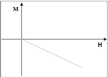
Figure I.3 The magnetization field of a diamagnetic material as a function of

magnetic field intensity. ... 4

Figure I.4 (a) A microscopic view of a demagnetized paramagnetic material;

(b) a microscopic view of a magnetized paramagnetic material. ... 5

Figure I.5 The susceptibility of a paramagnetic material as a function of: (a)

magnetic field intensity,(b) temperature. ... 5

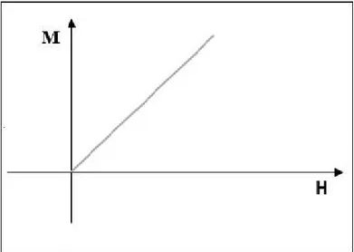
Figure I.6 The magnetization field of a paramagnetic material as a function

of magnetic field intensity... 6

Figure I.7 (a) A microscopic view of a demagnetized ferromagnetic

material; (b) a microscopic view of a magnetized ferromagnetic material. ... 7

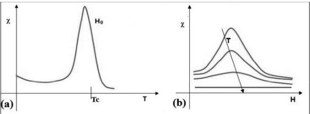
Figure I.8 The hysteresis loop of a ferromagnetic material. ... 7 Figure I.9 The susceptibility of a ferromagnetic material as a function of: (a)

temperature,(b) magnetic field intensity. ... 8

Figure I.10 The hysteresis loop of magnetization field as a function of

magnetic field intensity, in a ferromagnetic material... 8

Figure I.11 The entropy curves of a ferromagnetic material. Green line plots

the totally entropy whereas blue and red line represent the magnetic and the thermal contributions, respectively. ... 9

Figure I.12 The magnetocaloric effect detected as SMand Tadin a

ferromagnetic material where it is magnetized by magnetic field going from H0to H1. ... 11 Figure I.13 (a) The four processes of magnetic Ericsson cycle in T-S

diagram. (b) Principle of magnetic Ericsson cycle refrigerator. ... 14

Figure I.14 The four processes of magnetic Brayton cycle in S-T diagram.16 Figure I.15 The four processes of magnetic Carnot cycle in S-T diagram. 17

stages (I, II and III) are designed to have a different optimally adapted

material, whereas in case (b) they are produced with the same material. .... 18

Figure I.17 Overlaps in a cascade system lead... 19

to dissipation of energy and decrease the COP. ... 19

Figure I.18 The regeneration effect in the Brayton cycle... 20

Figure I.19 Typical A ... 22

Figure I.20 The four processes of AMR cycle in T-s diagram... 23

Figure I.21(a) First process of AMR cycle: adiabatic magnetization. ... 24

Figure I.21(b) Second process of AMR cycle: cold-to-hot side fluid flowing. ... 24

Figure I.21(c) Third process of AMR cycle: adiabatic demagnetization. ... 24

Figure I.21(d) Fourth process of AMR cycle: hot-to-cold end fluid flowing. ... 25

Figure I.22(a) First process of AMRR cycle with respect to the ... 26

... 26

Figure I.22(b) Second process of AMRR cycle with respect to the... 26

-to-hot flow. ... 26

Figure I.22(c) Third process of AMRR cycle with respect to the ... 27

... 27

Figure I.22(d) Fourth process of AMRR cycle with respect to the... 27

-to-cold flow. ... 27

Figure I.23 An example of the evaluation of relative cooling power based on the temperature dependence of magnetic entropy change, RCP(S). ... 29

Figure I.24 - SM(T) of single crystal of gadolinium parameterized for various magnetic field induction. ... 31

Figure I.25 Tad(T) of single crystal of gadolinium measured under different values of magnetic field induction... 31

Figure I.26 Heat capacity of single-crystal of gadolinium measured under different magnetic field induction. ... 32

Figure I.27 Tad(H,T) of in single crystal of gadolinium measured, during adiabatic magnetization and demagnetization, under a magnetic field induction which varies in 0÷1.5 T... 33

Figure I.28 (B,T) of in single crystal of gadolinium. ... 33

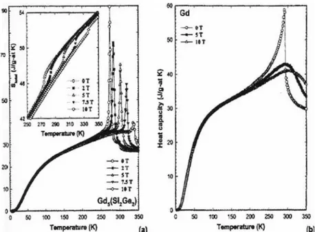
Figure I.29 - SM(H,T) of Gd5(Si2Ge2) parameterized for different magnetic field induction and compared with gadolinium... 35

Figure I.30 Tad(H,T) of Gd5(Si2Ge2), in comparison with Gd, for magnetic field inductions which change from 0 to 2 and from 0 to 5 T. ... 35

Figure I.31 The heat capacity of Gd5(Si2Ge2) as a function of temperature and magnetic field (a) in comparison with that of pure Gd (b). The inset in (a) shows total entropy of Gd5(Si2Ge2) as a function of temperature and magnetic field, as determined from the heat capacity. ... 36

magnetic field induction... 37

Figure I.33 Tad(H,T) of LaFe11.384Mn0.356Si1.26H1.52, for magnetic field

inductions which change from 0 to 0.4 T, 0.8T and 1.2 T. ... 38

Figure I.34 The heat capacity of LaFe11.384Mn0.356Si1.26H1.52as a function of

temperature and for different magnetic field change. ... 38

Figure I.35 - M(H,T) of LaFeCoSi compounds under 1T as magnetic

field induction, compared with a commercial Gd sample. ... 39

Figure I.36 Tad(H,T) of LaFeCoSi compounds for magnetic field

inductions which change from 0 to 1 T... 40

Figure I.37 The heat capacity of LaFeCoSi compounds as a function of

temperature under 1 T, compared with commercial gadolinium ... 40

Figure I.38 Isothermal entropy change Isothermal entropy change ( - S) for

MnFeP0.45As0.55. The dotted, solid and dashed lines correspond to a magnetic

field induction from 0 to 1.45 T, from 0 to 2 T and from 0 to 5 T

respectively. ... 41

Figure I.39 Adiabatic temperature change ( Tad) for MnFeP0.45As0.55for a

magnetic field induction from 0 to 1.45 T (dotted line), from 0 to 2 T (solid line) and from 0 to 5 T (dashed line)... 42

Figure I.40 MnFeP0.45As0.55heat capacity, evaluated under a magnetic field

induction varying from 0 to 1 T ... 43

Figure I.41 Isothermal entropy change Isothermal entropy change ( S) for

Pr0.65Sr0.35MnO3, resulting from the analysis of magnetization and heat

... 44

Figure I.42 Adiabatic temperature change ( Tad) for Pr0.65Sr0.35MnO3,

measured for a field change of 1T... 44

Figure I.43 Cp (H,T) measured forPr0.65Sr0.35MnO3,measured for a field

induction rising (red line) and falling (black line) in 0÷1 T range. ... 45

Figure I.44 - M

magnetic field induction, for the presented magnetocaloric materials. ... 46

Figure I.45 ad .5T as

magnetic field induction, for the presented magnetocaloric materials. ... 47

Figure II.1 Picture of 8Mag. ... 50 Figure II.2 Side view of the 8Mag magnetic system. ... 51 Figure II.3 (a) 8Mag core details: 1)permanent magnet assembly;

2)mounting support; 3)shaft-rotary valve combination; 4)regenerator; 5)magnetocaloric wheel; 6)fluid manifold to/from regenerators; 7)fluid manifold to/from heat exchanger; 8)bearings; 9)adjustable rings. ... (b) Longitudinal (A-A) and axial section (B-B) of the device core. ... 52

Figure II.4 Halbach array configuration adopted in 8Mag (longitudianl

section) ... 53

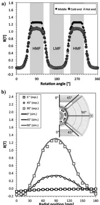
Figure II.5 (a) Measured flux density as a function of the rotation angle at

three radial positions: Hot end (200 mm); middle end (177.5 mm); cold end (155 mm). (b) Flux density as a function of the radial position for three

(exp.), whereas the lines report the simulated values (sim.). Zero is not the symmetry axis but the inner diameter of the magnetic system. The cold end of the regenerator is located at 65 mm, and the hot end is located at 110 mm.

... 54

Figure II.6 Equivalent hydraulic circuit: VH,Dis the valve connected with the hot end of the demagnetized regenerators; VC,Dis the valve connected with

the cold end of the demagnetized regenerators; VH,Mis the valve connected

with the hot end of the magnetized regenerators; VC,Mis the manifold

connected with the cold end of the magnetized regenerators. R0° and R180° are the magnetized regenerators, hydraulically in parallel flow; R90° and R270° are the demagnetized regenerators hydraulically coupled to R0° and R180°, also in parallel flow. ... 56

Figure II.7 Regenerator details: 1)shell, 2)diffuser, 3)magnetocaloric

material, 4)push-in fitting... 58

Figure II.8 A scheme of the experimental apparatus employed for

investigating the energy performances of 8Mag. ... 60

Figure II.9 The modified Ergun correlation. Comparison between the

experimental data (exp.) and predicted data from Eq. (II.6) (corr.). ... 64

Figure II.10 Sample of the pressure measurement at the ends of a

regenerator as a function of the rotation angle (fluid flow rate = 7 l/ min and fAMR = 0.71 Hz) ... 65

Figure II.11 ( AMRas a function of the heat rejection temperature for AMRas a function of the utilization

factor for different heat rejection temperatures. ... 67

Figure II.13 lossas a function of the utilization factor for different heat

rejection temperatures. ... 68

Figure II.14 spanas a function of the thermal load for different

frequencies and different fluid flow rates... 71

Figure II.15 spanas a function of fAMRfor different thermal loads

and different fluid flow rates ... 73

Figure II.16 spanfor three different couples of fluid

flow rate and fAMRcorresponding to the same utilization factor. ... 75

Figure II.17 The mechanical t spanfor three

different couples of fluid flow rate and fAMRcorresponding to the same

utilization factor. ... 76

Figure II.18 spanfor three different couples of fluid

flow rate and fAMRcorresponding to the same utilization factor. ... 77 Figure II.19 COP as a function of for three different couples of fluid flow rate and fAMRcorresponding to the same utilization factor. ... 77 Figure II.20 Cooling power as a function of temperature span for two

reservoir temperature... 80

Figure III.1 The packed bed AMR regenerator geometry: a 20x45mm2 wrapper contains 3600 spheres. ... 84

Figure III.2 The function Csp,magn(B,Ts) for gadolinium during magnetization under a 0÷1.2 T magnetic field induction. ... 90

Figure III.3 The function Csp,demagn(B,Ts) for gadolinium during demagnetization under a 1.2÷0 T magnetic field induction. ... 90

Figure III.4 The function Qmagn s) for gadolinium during magnetization under a 0÷1.2 T magnetic field induction... 91

Figure III.5 The function Qdemagn s) for gadolinium during demagnetization under a 1.2÷0 T magnetic field induction. ... 91

Figure III.6 Fluid velocity field in the regenerator: velocity field x component [m/s]. Phase of the cycle: fluid flow toward hot heat exchanger (from left to right side). Condition of operation: fAMR=1.79 Hz. TH= 298 K. ... 92

Figure III.7 Temperature field in the regenerator during magnetization. Condition of operation: fAMR= 1.79 Hz. TH= 298 K. ... 93

Figure III.8 Temperature field in the regenerator during isofield heating. Condition of operation: fAMR= 1.79 Hz. TH= 298 K. ... 93

Figure III.9 Pressure field in the regenerator during the blow phase. Fluid flows toward hot heat exchanger (from left to right side). ... 94

Figure III.10 Pressure drop estimated across the regenerator during an entire AMR cycle. ... 94

Figure III.11 Comparison between experimental and simulation results in terms of temperature span TAMRas a function of THat fAMRof (a)1.08, (b)1.25, (c)1.61 and (d)1.79. ... 97

Figure III.12 (a) Csp,magnand (b) Csp,demagnof Gd5(Si2Ge2)... 101

Figure III.13 (a) Csp,magnand (b) Csp,demagnof LaFe11.384Mn0.356Si1.26H1.52. 101 Figure III.14 (a) Csp,magnand (b) Csp,demagnof LaFe11.05Co0.94Si1.01. ... 102

Figure III.15 (a) Csp,magnand (b) Csp,demagnof MnFeP0.45As0.55... 103

Figure III.16 (a) Csp,magnand (b) Csp,demagnof Pr0.65Sr0.35MnO3. ... 103

Figure III.17 (a) Q,magnand (b) Q,demagnof Gd5(Si2Ge2)... 105

Figure III.18 (a) Q,magnand (b) Q,demagnof LaFe11.384Mn0.356Si1.26H1.52... 105

Figure III.19 (a) Q,magnand (b) Q,demagnof LaFe11.05Co0.94Si1.01. ... 106

Figure III.20 (a) Q,magnand (b) Q,demagnof MnFeP0.45As0.55. ... 107

Figure III.21 (a) Q,magnand (b) Q,demagnof Pr0.65Sr0.35MnO3. ... 107

Figure III.22 Tspanmeasured for the tested materials as a function of TH and compared with gadolinium. ... 109

Figure III.23 evaluated for the tested materials as a function of TH. ... 110

Figure III.24 COP estimated for the tested materials as a function of TH. 111 Figure III.25 COP as a function of the hot heat exchanger temperature. . 115

LaFe11.05Co0.94Si1.10, MnFeP0.45As0.55and Pr0.65Sr0.35MnO3as a function of the

hot heat exchanger temperature... 116

Figure III.27 The packed bed AMR regenerator geometry: a 20x45mm

wrapper contains 3600 spheres... 119

Figure III.28 The parallel plate AMR regenerator geometry: a 20x45mm

wrapper contains 27 plates and 26 channels... 119

Figure III.29 spanevaluated for both the regenerator configuration for

variable fluid flow velocity and therefore fluid flow rate ... 121

Figure III.30 The refrigeration power evaluated for both the regenerator

configuration for variable fluid flow velocity and therefore fluid flow rate. ... 121

Figure III.31 The refrigeration power evaluated for both the regenerator

configuration for variable fluid flow velocity and therefore fluid flow rate. ... 122

Figure III.32 The work of the secondary fluid circulation pump reported

Index of Tables

Table I.1 Physical and MCE characteristics of magnetocaloric materials in

the room temperature range... 45

Table I.2 A comparison among magnetocaloric materials ... 46

in terms of relative cooling powers and costs. ... 46

Table II.1 Performances of the magnetic ... 55

system for different height of air gap. ... 55

Table II.2 DC Motor and planetary gearhead combination data... 58

Table II.3 Characteristics of the sensors used and the accuracy of the measurements performed. ... 61

Table II.4 Error propagation analysis. (*) It has been assumed depending both on the accuracy of the pressure gauges and on the accuracy of the assumed depending both on the accuracy of the tesla meter and on the accuracy of the thermocouple. ... 64

Table II.5 Utilization factor corresponding to the AMR cycle frequency at different TH. The specific heat of gadolinium is assumed equal to 381 J/kg K. ... 66

Table II.6 Pressure drops at different fluid flow rates... 70

Table III.1 Mathematical expression of Cspfound for the presented materials during magnetization (Csp,magn) and demagnetization (Csp,demagn)... 100

Table III.2 materials during magnetization (Qmagn demagn ... 104

Abstract

Magnetic refrigeration is an innovative, promising and ecologic technology, which aims to substitute the conventional vapor-compression refrigeration by the employment of solid materials as refrigerants instead of the fluid-state ones, own of vapour compression refrigeration. This emerging technology bases its operation on the magnetocaloric effect (MCE), which is a physical phenomenon, related to solid-state materials with magnetic properties. The magnetic field causes an entropy change due to magnetic ordering. The maximum MCE occurs near the magnetic ordering temperature, which is recognized as the Curie temperature of a ferromagnetic material. For materials displaying simple magnetic ordering (i.e. paramagnetic to ferromagnetic phase transformations) a rapid increase in magnetic field causes a temperature rise in the material; likewise, a rapid reduction in the field causes cooling. This variation in temperature is called adiabatic temperature change which is a function of the magnetic field intensity and of the initial temperature.

To reach a useful temperature span it is required employing a regenerative thermodynamic cycle. In 1982, the employment of a reciprocating thermal regenerator coupled with magnetocaloric cycle has been shown: it was introduced the Active Magnetic Regenerative refrigeration cycle, well known as AMR cycle. The innovative idea leads to a new magnetic cycle, different from the previous ones (Carnot, Ericsson, Brayton, or Stirling). It considers a magnetic Brayton cycle but the main innovation consists of introducing the AMR regenerator concept, i.e. the employment of the magnetic material itself both as refrigerant and as regenerator. A secondary fluid is used to transfer heat from the cold to the hot end of the regenerator. Substantially every section of the regenerator experiments its own AMR cycle, according to the proper working temperature. Through an AMR one can appreciate a larger temperature span among the ends of the regenerator.

Active Magnetic Regenerator is the core of a magnetic refrigerator system. The performance of an AMR system strongly depends on the magnetocaloric effect of the magnetic material used to build the regenerator, on the geometry of the regenerator and on the secondary fluid.

the research, treated during the PhD period. The personal contribution in the research field of magnetic refrigeration has combined both the numerical and the experimental research that have been done hand in hand.

At the Refrigeration Lab (LTF) of University of Salerno, the first Italian prototype of a Rotary Permanent Magnet Magnetic Refrigerator (RPMMR) has been projected and developed (Aprea et al., 2014), whose name is 8Mag and presents a rotating magnetic group whereas the magnetocaloric material (MCM) is stationary. Gadolinium has been selected as magnetic refrigerant and demineralized water has been employed as heat transfer fluid.

In the present thesis, the experimental tests conducted on the RPMMR have been presented, with the purpose to investigate the energy performances of the device, like temperature span, refrigerating power and COP, when the system was subjected to different operating conditions obtained by varying the cycle operating frequency, the thermal load, the volumetric flow rate of the auxiliary fluid and the temperatures of the cold and hot heat exchangers. In particular, the results of three different campaigns of tests are presented: 1) a primary campaign based on zero load tests; then two other campaigns have been conducted in order to explore the energetic performances of 8Mag: 2) by changing the cycle frequencies, the cooling load and fluid flow rate, while the hot side temperature was fixed, in order to give an overview of the performances and to underline an optimal operating frequency, for each set of operating conditions. 3) Fixing flow rate and AMR cycle frequency to the optimal value, a further investigation has been conducted by varying cooling load.

A two-dimensional numerical model of a packed bed- AMR regenerator has been developed, as primary purpose, to operate according to the prototype, since the model replicates the thermo-fluid-dynamical behavior of one of the RPMMR's regenerators, including the magnetocaloric effect acting into the solid refrigerant. To this aim, the model has been experimentally validated with experimental results provided by the prototype. This model has been used to optimize the experimental device and to identify significant areas of device improvement. Thus, it has been used to explore the critical aspects of 8Mag and to outline the way to improve performances. Anyway, the model has been easily generalized to consider different device geometries, temperature spans, secondary fluids, and magnetic materials. As a matter of fact, in this thesis are shown the results obtained investigating, through the model, the effect of other different magnetocaloric materials when they act as refrigerant employed in one of the AMR regenerator of the prototype. Moreover, the environmental impact in terms of greenhouse effect has also been investigated, by comparing the performances of the RPMMR with the one of a vapor compression plant in terms of TEWI index (Total Equivalent Warming Impact).

Introduction

Nowadays, the refrigeration is responsible of more than 17% of the overall energy consumption all over the world and most modern refrigeration units are based on Vapor Compression Plants (VCP). The traditional refrigerant fluids employing VCP, i.e. CFCs and HCFCs, have been banned by the Montreal Protocol in 1987 (Montreal Protocol, 1987), because of their contribution to the disruption of the stratospheric ozone layer (Ozone-Depleting Potential substances ODPs). Over time it has been following periodical meetings among the Parties to the Montreal Protocol. Since 2000 the usage of HCFCs in new refrigerating systems was forbidden, letting HFCs the only fluorinated refrigerants allowed because of their zero ODP characteristic. Since 2009, each meeting related to Montreal protocol, initially dedicated to the phase-out of the substances depleting the stratospheric ozone layer, namely CFCs and HCFCs, had been leading to conflicting exchanges on high Global Warming Potential HFCs which replace CFCs and HCFCs most of the time. Year after year, human activities have been increasing the concentration of greenhouse gases in the atmosphere, thus resulting in a substantial warming of both earth surface and atmosphere. The impact of greenhouse gases on global warming is quantified by their GWP (Global Warming Potential). Thus, over the year measures to reduces global warming have been taken, beginning with the Kyoto Protocol (Kyoto Protocol, 1997) and consequently with the EU regulations applying the prescriptions derived from it, like EU regulation 517/2014 (EU No 517/2014) on fluorinated greenhouse gases.

The above described general frameworks led scientific community to studying and applying (Aprea et al., 2012; Palm, 2008) resolutions with environmentally friendly gases, with small GWP and zero ODP: one of the most focused classes of new generation refrigerants is hydrofluoroolefins (HFO) (Aprea et al., 2016a; Mota-Babiloni et al., 2016), descending of olefins rather than alkanes (paraffins) and they are known as unsaturated HFCs, with environmentally friendly behavior, quite low costs. Despite all these advances, it is essential to underline that a vapor compression plant produces both a direct and an indirect contribution to global warming. The former depends on the GWP of refrigerant fluids and on the fraction of

operation and maintenance, or is not recovered when the system is scrapped. The indirect contribution is related to energy-consumption of the plant. In fact, a vapor compression refrigerator requires electrical energy produced by a power plant that typically burns a fossil fuel, thus releasing CO2 into the

atmosphere. The amount of CO2emitted is a strong function of the COP of

the vapor compression plant.

For all these reason, in the last decades the interest of scientific community has oriented itself in studying and developing new refrigeration technologies of low impact in our ecosystem: a class of them is composed by solid-state cooling (Kitanovski and Egolf, 2006; et al., 2014; et al., 2015), which are gaining more and more attention, due to their potential in being performing and ecological methodologies. Recent discoveries of giant caloric effects (Pecharsky and Gschneidner, 1997; Lu et al., 2010; Liu et al., 2014) in some ferric materials have opened the door to the use of solid-state materials as an alternative to gases for conventional and cryogenic refrigeration.

Actually, the most promising, eco-friendly, emerging solid-state technique is constituted by magnetic refrigeration (MR) (Kitanovski et al., 2016), whose main innovation consists in employing solid materials with magnetic properties as refrigerants, able to increase or decrease their temperature when interacting with a magnetic field. Instead of the fluid refrigerants, proper of vapour compression, a magnetic refrigerant is a solid and therefore it has essentially zero vapour pressure, which means no direct ODP and zero GWP.

Specifically, magnetic refrigeration is related to magnetocaloric effect (MCE) (Warburg, 1881), a physical phenomenon observed in some material with magnetic properties and it consists in an increment of temperature in the MCE material because of material's magnetization under adiabatic conditions. A regenerative Brayton based thermodynamical cycle, called Active Magnetic Regenerative refrigerant (AMR) cycle, is the one where magnetic refrigeration founds its operations. Therefore, Active Magnetic Regenerator is the core of a magnetic refrigerator system. It is a special kind of thermal regenerator made of material with magnetic properties, which works both as a refrigerant and as a heat regenerating medium. The performance of an AMR system strongly depends on the magnetocaloric effect of the magnetic material used to build the regenerator, on the geometry of the regenerator and on the operating conditions of the system. The cooling efficiency in magnetic refrigerators can reach 60% of the theoretical limit, as compared to the 40% achieved by the best vapor compression plant.

At the Refrigeration Lab (LTF) of University of Salerno, the first Italian prototype of a Rotary Permanent Magnet Magnetic Refrigerator (RPMMR)

(MCM) is stationary. Gadolinium has been selected as magnetic refrigerant and demineralized water has been employed as heat transfer fluid. The total mass of gadolinium (1.20 kg), shaped as packed bed spheres, is housed in 8 regenerators. A magnetic system, based on a double U configuration of permanent magnets, provides a magnetic flux density of 1.25 T with an air gap of 43 mm. A rotary vane pump forces the regenerating fluid through the regenerators.

The present thesis aims to explore, report and explain all the aspects of the research, treated during the PhD period. The personal contribution in the research field of magnetic refrigeration has combined both the numerical and the experimental research that have been done hand in hand.

A two-dimensional numerical model of a packed bed- AMR regenerator has been developed, as primary purpose, to operate according to the prototype, since the model replicates the thermo-fluidodynamic behavior of one of the RPMMR's regenerators, including the magnetocaloric effect acting into the solid refrigerant. To this aim, the model has been experimentally validated (Aprea et al., 2015a) with experimental results provided by the prototype. This model has been used to optimize the experimental device and to identify significant areas of device improvement. Thus, it has been used to explore the critical aspects of 8Mag and to outline the way to improve performances. Anyway, the model has been easily generalized to consider different device geometries, temperature spans, secondary fluids, and magnetic materials. To this purpose, the model has been tested when employing new magnetocaloric materials (Aprea et al., 2015b), whose performance have been also compared (Aprea et al., 2015c), from an environmental point of view, with the ones of a commercial vapor-compression refrigerator working with R134a. Moreover, additional investigations have been conducted to explore the behavior of the regenerator with a parallel-plate configuration (Aprea et al., 2016b), employing a number of different magnetocaloric materials.

As a matter of fact, in this thesis are shown the results obtained investigating (Aprea et al., 2015b), through the model, the effect of other different magnetocaloric materials when they act as refrigerant employed in one of the AMR regenerator of the prototype. Different magnetic materials have been considered as refrigerant: second order phase magnetic transition materials, like pure gadolinium, Pr0.45Sr0.35MnO3 and first order phase

magnetic transition alloys Gd5(SixGe1-x)4, LaFe11.384Mn0.356Si1.26H1.52,

LaFe11.05Co0.94Si1.10 and MnFeP0.45As0.55. Such materials have also been

object of an additional investigation (Aprea et al., 2016b) related to the evaluation of the performances between two different geometries of the AMR regenerator: packed-bed and parallel-plate. Moreover, the environmental impact in terms of greenhouse effect has also been investigated, by comparing (Aprea et al., 2015c) the performances of the

(Total Equivalent Warming Impact). A vapor compression plant (VCP) produces both a direct and an indirect contribution to global warming, whereas an AMR cycle has only an indirect effect. The analysis has been performed comparing the VCP and the magnetic refrigerator when the latter is working with several different magnetocaloric refrigerants.

Furthermore, are also presented the experimental tests conducted (Aprea et al, 2016c) on the RPMMR, with the purpose to investigate the energy performances of the device, like temperature span, refrigerating power and COP, when the system was subjected to different operating conditions obtained by varying the cycle operating frequency, the thermal load, the volumetric flow rate of the auxiliary fluid and the temperatures of the cold and hot heat exchangers. The results of three different campaigns of tests are presented: 1) a primary campaign based on zero load tests; then two other campaigns have been conducted to explore the energetic performances of 8Mag: 2) by changing the cycle frequencies, the cooling load and fluid flow rate, while the hot side temperature was fixed, in order to give an overview of the performances and to underline an optimal operating frequency, for each set of operating conditions. 3) Fixing flow rate and AMR cycle frequency to the optimal value, a further investigation has been conducted by varying cooling load.

Chapter I

Magnetic refrigeration:

generalities

I.1 Magnetocaloric effect

Magnetocaloric effect is an intrinsic property of all solid-state materials, due to the coupling between the magnetic spin and the crystal lattice with an external magnetic field whom produces a change in magnetic entropy contribution. When the material is magnetized there will be some ordering of the magnetic spins, forcing them towards the direction of the applied field. If this is done isothermally, this will reduce

M). On the other side, if the magnetization

is done adiabatically, without any thermal interaction with the external ambient, the total sample entropy remains constant and the decrease in magnetic entropy is countered by an increase in the lattice and electron entropy. This causes a heating of the material and a temperature increase

ad). The inverse procedure

also applies: under adiabatic demagnetization the magnetic entropy increases, causing a decrease in lattice vibrations and by that a temperature decrease.

I.1.1 Historical background

MagnetoCaloric Effect (MCE) is a physical phenomenon discovered casually in 1881 by Emil Gabriel Warburg, a German professor of Physics at University of Strasbourg, during some experiments on ferromagnetic materials. Warburg observed (Warburg, 1881) a slight increment of temperature when the material was subjected to a huge magnetic field whereas, once it was extracted from the field, its temperature suffered a decrease. Cryogenic temperatures have been the first branch of refrigeration

where MCE found application, since 1920 (Debye, 1926; Giauque, 1927). It is maturely used in liquefaction of hydrogen and helium.

The research on room temperature magnetic refrigerators has taken place since 1976 with the first prototype developed by Brown at the NASA Lewis Research Centre (Brown, 1976). In 1982, the employ of a reciprocating thermal regenerator coupled with magnetocaloric cycle has been shown. It is well known as Active Magnetic Regenerator (AMR) (Barclay, 1982). Since then an appreciable number of AMR-based experimental prototypes have been developed, with a different configuration of regenerators, different magnetic materials and different magnetic source (Yu et al., 2010; Tomc et al., 2013; et al., 2013; Vuarnoz and Kawanami, 2013; Engelbrecht and Pryds, 2014; Jotani et al., 2014). Nevertheless, most of the experimental devices don't provide yet results in terms of energetic performances, cooling power and temperature span as satisfactory as being comparable with the one provided by vapor compression systems.

I.1.2 Magnetic substances and their classification

Every material able to interact with a magnetic field and therefore characterized by magnetic properties, belongs to the magnetic substances. A magnetic substance is conceivable as a collection of small magnetic dipoles, associated with its atomic characteristics that are oriented casually. If the substance interacts with an external magnetic field, whom is characterized by an intensity H>0, the dipoles orient themselves in the same direction of the field and the substance is magnetized. M is the magnetization field and is defined as the magnetic moment of the substance per unit of volume:

(I.1) where miis the magnetic moment related to the ithmolecule of the substance

contained in the volume V.

It is possible relating M and the magnetic field H as:

(I.2) agnetic susceptibility of the substance and it is dimensionless.

The relation between the magnetic field induction B and the magnetic field H is given by:

(I.3) ses the attitude of the material in being magnetized. The magnetic permeability can

(I.4) where r is the relative permeability index, depending on the magnetic

substance.

The magnetic permeability and the magnetic susceptibility are related by the following relationship:

(I.5) Therefore, considering (I.5) and (I.2), (I.3) could be also expressed as:

(I.6) The magnetic substances are classifiable in:

a) diamagnetic; b) paramagnetic; c) ferromagnetic.

The diamagnetic materials, when come under the action of an external magnetic field H, see their dipoles ordering in opposition to H; the associated magnetization field M has opposite direction of H. Therefore, a diamagnetic material tends to weaken the external field, as shown in figure I.1.

Figure I.1 (a) A microscopic view of a demagnetized diamagnetic material; (b) a microscopic view of a magnetized diamagnetic material.

The susceptibility of diamagnetic materials is always negative and non-depending both by temperature and by the magnetic field intensity, as shown in figures I.2(a) and I.2(b). Thus, the function which relies M and H is linearly decreasing, as plotted in figure I.3.

The most common diamagnetic materials are water, most of organic substances and some metals like mercury, gold, silver, copper and bismuth. For all of them, magnetic susceptibility belongs to -10-4_÷-10-6_range.

Figure I.2 The susceptibility of a diamagnetic material as a function of: (a) temperature,(b) magnetic field intensity.

Figure I.3 The magnetization field of a diamagnetic material as a function of magnetic field intensity.

A magnetic substance is defined paramagnetic if, when it is under the action of an external magnetic field H, its dipoles orient themselves in the same direction of the field; the associated magnetization field M tends to strengthen H, since the two field are in phase, as shown in figure I.4.

Figure I.4 (a) A microscopic view of a demagnetized paramagnetic material; (b) a microscopic view of a magnetized paramagnetic material.

independent by the external magnetic field. Moreover,

temperature increases, because thermal agitations and lattice vibrations hinder the alignment of the magnetic moments of the atoms, in the H direction. The relationship between susceptibility and temperature, in paramagnetic materials is called 1stCurie law and is given by:

(I.7) where C is called Curie constant and its value depends of the material. temperature, respectively.

Figure I.5 The susceptibility of a paramagnetic material as a function of: (a) magnetic field intensity, (b) temperature.

As a result, M and H are bound by a linearly increasing function, as reported in figure I.6. The most common paramagnetic materials are aluminium, platinum, magnesium, calcium, sodium, oxygen and uranium. For all of them, magnetic susceptibility belongs to 10-4_÷10-5_{range, at room}

temperature.

Figure I.6 The magnetization field of a paramagnetic material as a function of magnetic field intensity.

Ferromagnetic are all the materials whose susceptibility is strongly dependent by both the temperature and the applied magnetic field. Moreover, a ferromagnetic material is able to keep the magnetic moment even when the magnetizing field has been removed. The lattice structure of ferromagnetic materials is composed by a number of subdomains where the dipoles contained in, are locally aligned in the same direction. When a magnetizing filed is applied, all the dipoles of all the subdomains are arranged in

magnetization, as shown in figures I.7(a) and I.7(b). The energy spent to demagnetize the material manifests itself in a delay in response, said hysteresis. Moreover, the correspondence between magnetic field induction

B and the applied magnetic field H is regulated by the hysteresis loop,

reported in figure I.8, which represents the state diagram of the ferromagnetic material. The shape of the hysteresis loop strongly depends by applied field.

Figure I.7 (a) A microscopic view of a demagnetized ferromagnetic material; (b) a microscopic view of a magnetized ferromagnetic material.

Figure I.8 The hysteresis loop of a ferromagnetic material.

nd_{Curie law}

(also called Curie-Weiss law), visible in figure I.9(a), as follows:

(I.8) TC

and above which, the material assumes a paramagnetic behaviour. Thus, the Curie temperature is also the temperature where the ferromagnetic to

paramagnetic transition takes place. The dependence of the susceptibility with the magnetic field is plotted in figure I.9(b).

Figure I.9 The susceptibility of a ferromagnetic material as a function of: (a) temperature, (b) magnetic field intensity.

As a result, also the dependence of between the magnetization and the field is not linear anymore but regulated by the hysteresis loop, as illustrated in figure I.10.

Figure I.10 The hysteresis loop of magnetization field as a function of magnetic field intensity, in a ferromagnetic material.

Some materials which belong to the ferromagnetic class are gadolinium, iron, nickel, as well as several iron-based alloys.

I.1.3 The entropy

Entropy S

of measure in the international measurement system is Joule divided by Kelvin [J/K].

The entropy of a magnetic substance depends both by the temperature and the magnetic field and it is composed by three terms:

(I.9) The first contribution SL(T) is called vibrational entropy since considers

the disorder of the material due to the increase of lattice vibrations, when the system is supplied energy as heat. The heat supplying takes to another term of disorder: SL(T), the electronic entropy, which measure the disorder of

system due to the increasing randomness of the electronic spins. The third contribution SM(T,H), called magnetic entropy, is related both to temperature

and magnetic field. When the magnetic material goes under the presence of an external magnetic field, its magnetization takes the dipoles aligning with the field e therefore an increment of magnetic order, as well as a reduction of

SM(T,H). Dually, when the external field is removed, the random disposition

of the dipoles led to an increase of magnetic entropy. Figure I.11 plot the entropy curves of a ferromagnetic substance, together with the trends of the single contributions.

Figure I.11 The entropy curves of a ferromagnetic material. Green line plots the totally entropy whereas blue and red line represent the magnetic and the thermal contributions, respectively.

I.1.4 Heat capacities in magnetic materials

The heat capacity related to a generic process where the z parameter remains constant is:

(I.10) Considering the second law of thermodynamic for a reversible process:

(I.11) the (I.10) becomes:

(I.12) In analogies with heath capacity at constant pressure and volume, for magnetic materials is interesting to consider the heat capacity at constant magnetic field and the heat capacity at constant magnetization, respectively defined as:

(I.13)

(I.14) In the class of ferromagnetic materials exhibits a peak at the Curie temperature of the material. Moreover, the temperature where the peak is located increases according to the intensity of the applied magnetic fields.

I.1.5 Magnetocaloric effect and magnetic transition materials

Magnetocaloric effect is a physical phenomenon, related to solid-state materials with magnetic properties. MCE consists in a coupling between the entropy of the Magnetocaloric Material (MM) and the variation of an external magnetic field applied to the material, which causes magnetic ordering in the MM structure. If the magnetization is done isothermally, it will decrease the magnetic entropy of the material, by the isothermal entropy change SM and, therefore, a change in the total entropy of the magnetic

material is registered.

On the other side, if the magnetization occurs in an adiabatic process, without any interaction with the external environment, the total entropy of MM remains constant and the consequent decreasing in magnetic entropy is countered by an increase in the lattice and electron entropy contributions. This causes a heating of the material and a temperature increase given by the

quantities SM and Tad during an adiabatic magnetization of a

ferromagnetic material.

Figure I.12 The magnetocaloric effect detected as SM and Tad in a

ferromagnetic material where it is magnetized by magnetic field going from H0to H1.

Dually, under adiabatic demagnetization the magnetic entropy increases, causing a reduction in lattice vibrations and therefore a temperature decrease. At its Curie temperature, where is located its own magnetic phase transition, a MM shows the peak of MCE, in terms of Tad and SM. This

occurs because the two opposite forces (the ordering force due to exchange interaction of the magnetic moments, and the disordering force of the lattice thermal vibrations) are approximately balanced near the Curie point TC.

Hence, the isothermal application of a magnetic field produces a much greater increase in the magnetization (i.e., an increase of the magnetic order and, consequently, a decrease in magnetic entropy, SM) near the Curie

point, rather than far away from Tc. The effect of magnetic field above and

below Tcis significantly reduced because only the paramagnetic response of

the magnetic lattice can be achieved for T Tc, and for T Tc the

spontaneous magnetization is already close to saturation and cannot be increased much more. Similarly, the adiabatic application of a magnetic field leads to an increase in the magnetic material temperature, Tad, which is also

sharply peaked near the Tc.

The two possible magnetic phase changes that one can observe at the Curie point are First Order Magnetic Transition (FOMT) and Second Order Magnetic Transition (SOMT). At the Curie point a magnetic transition has FOMT characteristics when the material exhibits a discontinuity in the first derivative of the Gibbs free energy (G.f.e.), magnetization function, whereas

has a SOMT behavior when the gap is detected in the second derivative of G.f.e., magnetic susceptibility, while its first derivative is a continuous function. Most of the magnetic materials order with a SOMT from a paramagnet to a ferromagnet, ferrimagnet or antiferromagnet.

Considering an internally reversible process, the MCE for SOMT materials can be evaluated as:

(I.15) (I.16) For that reason, in a SOMT material, while exhibits its maximum value, one can register the peak of MCE, located at the Curie temperature or near absolute zero, respectively if the material is a ferromagnetic or paramagnetic. Instead in a FOMT material, the phase transition should ideally take place at constant temperature for an infinite value of resulting a giant magnetocaloric effect. The FOMT materials exhibit both an instantaneous orientation of magnetic dipoles and a latent heat correlated with the transition. Moreover, in some FOMT materials it is possible observing a coupled magnetic and crystallographic phase transition. Thus, in this case, applying a magnetic field to these FOMT materials, can produce both the magnetic state transition from a paramagnet or an antiferromagnet to a ferromagnet, simultaneously with a structural variation or a significant phase volume discontinuity but without showing a clear crystallographic alteration. Since that partial first derivatives of G.f.e. regarding T or H present a discontinuity at the first order phase transition, the bulk magnetization varies by M and CHideally has an infinite value at

the Curie temperature. Therefore, the isothermal magnetic entropy change ( SM) in a FOMT material can be estimated by (I.17) coming from the

Clasius-Clapeyron equation:

(I.17) where the derivative is kept at equilibrium.

The discovery of giant magnetocaloric effect in Gd5(Si4-xGex), reported

by Pecharsky and Gschneidner in 1997 (Pecharsky and Gschneidner Jr., 1997), stimulated a considerable growth of research to both find new materials where the effect is just as potent and to understand the role of magneto-structural transitions play in its enhancement. Giant MCE in FOMT materials, already observed, comes out since it is the result of two phenomena: the conventional magnetic entropy-driven process (magnetic entropy variation ) and the difference in the entropies of the two

terms considers the greater contribution due to entropy variation in FOMT with respect to SOMT materials:

(I.18) Assuming constant, in a FOMT material could be estimated as:

(I.19) The peak of adiabatic temperature variation is greater in most of the FOMT than SOMT materials.

There are fundamental differences in the behavior of FOMT and SOMT materials:

in a first order transition the MCE is concentrated in a narrow temperature range, whereas in a second order the transition spread over a broad temperature range.

In a SOMT materials the adiabatic temperature variation is nearly immediate whereas it doesn't happen in FOMT materials because of the consequent alteration in their crystallographic structure, which produces a displacement of the atoms, needing thus of an amount of time required many orders of magnitude larger. The non-instantaneous response to the magnetic field of FOMT material, could become a significant problem since the operation frequencies usually adopted by magnetic refrigerators are in [0.5÷10] Hz range, where the delay in materials' answer could assume significant values.

A substantial hysteresis has generally been detected (Aprea et al, 2011a, 2011b) in FOMT materials, whereas it is very low in SOMTs. The consequences of hysteresis when analyzing the MCE are: i) history dependence: parameters such as magnetization and heat capacity now become non-single valued functions of temperature and field; ii) energy dissipation: heat is dissipated during the magnetization process, and the dissipation adds heat to the system.

The large volume variation that one can observe in FOMT materials is another defect that must be considered when deciding to employ these materials.

I.2 Thermodynamical cycles for magnetic refrigeration

Magnetic refrigerator completes cooling/refrigeration by magnetic material through magnetic refrigeration cycle. In general, a magnetic refrigeration cycle consists of magnetization and demagnetization in which

heat is expelled and absorbed respectively, and two other benign middle processes.

The basic cycles for magnetic refrigeration are magnetic Carnot cycle, magnetic Stirling cycle, magnetic Ericsson cycle and magnetic Brayton cycle (Yu et al., 2003; Kitanovski and Egolf, 2006,). Among them, the magnetic Ericsson and Brayton cycles are applicable for room temperature magnetic refrigeration. The employment of a regenerator in the Ericsson and Brayton cycles lets the achievement of a large temperature span and easy operating.

I.2.1 Magnetic Ericsson cycle

Ericsson cycle consists of two isothermal processes/ stages and two isofield processes as illustrated in figures I.13(a) and I.13(b).

Figure I.13 (a) The four processes of magnetic Ericsson cycle in T-S

1. In the isothermal magnetization process I(A B in Fig. I.13(a)), when magnetic field increases from H0 to H1the heat transferred

from magnetic refrigerant to the upper regenerator fluid

(I.20) makes the latter increasing its temperature.

2. In the isofield cooling process II ( in Fig. I.13(a)), while magnetic field is kept constant at the maximum value H1, both the

refrigerant and the magnet which generates the field move downward to bottom and hence the heat

(I.21) is transferred from magnetic refrigerant to regenerator fluid. Then a temperature gradient is set up in the regenerator.

3. In the isothermal demagnetization process III ( in Fig. I.13(a)), when magnetic field decreases from H1to H0, the magnetic

refrigerant absorbs heat:

(I.22) from the lower regenerator fluid. After that the fluid decreases its temperature.

4. In the isofield heating process IV (

magnetic field has kept constant at the minimum H0, both the

magnetic refrigerant and magnet move upward to the top and the regenerator fluid absorbs heat

(I.23) To make the Ericsson cycle possess the efficiency of magnetic Carnot cycle, it is required that the heat transferred in two isofield processes Qbc, Qda

are equal. S curves are optimal, that is, SMkeeps constant in the cooling temperature range.

I.2.2 Magnetic Brayton cycle

Magnetic Brayton cycle consists of two adiabatic processes and two isofield processes as shown in figure I.14.

Figure I.14 The four processes of magnetic Brayton cycle in S-T diagram.

The first process (A B in Fig. I.14) consists in and adiabatic magnetization, due to magnetic field increasing from H0to H1, that leads to a

temperature increment of Tad,ABin the solid refrigerant. With the field kept

constant at H1, in the isofield process ( in Fig. I.14) the heat of the area

BC14 is transferred from the refrigerant to the hot heat exchanger at temperature TH. In the adiabatic demagnetization ( in Fig. I.14) process

the applied magnetic field falls from H1 to H0 and the solid refrigerant

reduces its temperature of a quantity Tad,CD as a result of magnetocaloric

effect. In the isofield process at H0the heat of the area AD14 is subtracted

from the cold heat exchanger at TC. No heat flows from and out of the

magnetic refrigerant during the adiabatic magnetization and demagnetization processes.

The Brayton cycle can exhibit optimal performance as well with magnetic refrigerants having parallel T S curves.

I.2.3 Magnetic Carnot cycle

The magnetic Carnot cycle, consists of two adiabatic and two isothermal processes, applied to a magnetic refrigerant, as shown in figure I.15.

Figure I.15 The four processes of magnetic Carnot cycle in S-T diagram.

An adiabatic magnetization occurs in process

continues with a further magnetization in stage 2 3, which is now an isothermal magnetization. During this process generated heat is extracted from the system. The next process step, namely 3 , is an adiabatic demagnetization process. Connecting the system with a heat source leads to an isothermal demagnetiza .

It becomes clear that the Carnot cycle can only be run, if a minimum of four different magnetic fields occur, through which the magnetocaloric material is moved. In the vertical process 1 2 the alteration of the magnetic field has to be applied quickly, not allowing heat to diffuse away or be transported out by convection. In the isothermal magnetization requires an alteration of the magnetic field and simultaneous rejection of heat. This process will therefore be slower. The area between (1 2 3 4) represents the work required and the area (1 4 a b) is related to the thermal cooling energy.

I.3 Cascade systems regenerators

All the cycles previously discussed are ideal cycles. At present the existing magnetocaloric materials could do not show sufficiently wide temperature differences for some frequently occurring refrigeration and heat pump applications. A solution to this problem is to build magnetic

refrigerators and heat pumps, which take advantage of cascades. However, both the regeneration and the cascade systems show additional irreversibility in their cycles. These leads to lower coefficients of performance.

Cascade systems are well known from conventional refrigeration technology. A cascade system is a serial connection of some refrigeration apparatuses. They may be packed into one housing to give the impression of having only a single unit. Each of these apparatuses has a different working domain and temperature range of operation. This can be seen in Fig. I.16(a) by the decreasing temperature domains of stages I III. In this figure the cooling energy of stage I (surface: ef14) is applied for the heat rejection of stage II (surface cd23). Analogously, the cooling energy of stage II (surface cd14) is responsible for the heat rejection in stage III. The cooling energy of the entire cascade system is represented by the surface ab14 of the last stage (white domain). The total work performed in the total cascade system is given by the sum of the areas 1234 of all present stages I, II, and III.

Figure I.16 Two cascade systems based on the Brayton cycle. In case (a) all

stages (I, II and III) are designed to have a different optimally adapted material, whereas in case (b) they are produced with the same material.

The magnetocaloric effect is maximal at the Curie temperature. It is large only in the temperature interval around this temperature, with decreasing effect in the case of greater (temperature) differences. It is therefore, advantageous that the operating point of the refrigeration plant and this temperature interval of optimal magnetocaloric effect coincide. If the temperature span of the refrigeration process is too wide, a decrease in efficiency occurs. A solution to this problem is to work with a cascade system, where each internal unit has its own optimally adapted working temperature. Each stage of a cascade system contains a different magnetocaloric material (Fig. I.16(a)) or it contains the same (Fig. I.16(b)).

Figure I.17 Overlaps in a cascade system lead

to dissipation of energy and decrease the COP.

A major advantage of a magnetic refrigeration cascade system over a conventional one is that in the magnetic refrigeration machine no heat exchangers are required between the cooling process of the higher stage and the heat rejection process of the lower stage. This is since the magnetocaloric material is solid and a single fluid may be transferred to both stages.

I.4 The regenerators

The introduction of regenerators in refrigeration systems, with reference to magnetic refrigeration, has the purpose to recover heat fluxes involved in Brayton cycle, that otherwise would have gone lost. The approach is particularly needed in room temperature magnetic refrigeration, where the vibrational entropy contribution becomes too high to be neglected. cool the thermal load offered by the crystalline lattice, thus reducing the useful effect of the cycle. As a matter of fact, if a regenerator is added to the system, the heat rejected by the crystalline structure in one of the process of the cycle, is stored and then given back in the other process. By the way, the energy spent to cool the crystalline structure could be utilized effectively to increase of effective entropy change and temperature span (Yu et al., 2003).

Figure I.18 The regeneration effect in the Brayton cycle.

In figure I.18 one can appreciate the effect of the regeneration in Brayton cycle: thanks to the thermal interchange is possible to reach a temperature range TA-TC'greater than TA-TC, that would occur without regeneration, and

a higher entropy change.

It is useful underlining the characteristics proper of the different typologies of regenerator. There are three types of regenerators employable in magnetic refrigerators:

a) external, b) internal, c) active.

Heat transferring through external regenerator between the regenerator material (which generally is solid-state) and the magnetic refrigerant is completed by an auxiliary heat transfer fluid.

With internal regenerator solution, the magnetic refrigerant is placed in regenerator together with the regenerator material and heat is transferred directly between themselves so that the regenerator should be in the magnetic field area.