A CODE TO EVALUATE INVESTMENT
PROJECTS IN ENERGY SYSTEM WITH A SAM
AND A ENERGY-SAM
M. RAO, C. FERRARESE, M. SABETTA Fusion and Technology for Nuclear Safety
and Security Department Development of Particle Accelerators and MedicalApplications PhysicalTechnologies for Safety and Health Division
FrascatiResea
FrascatiResearch Centre,Rome,Italy
RT/2019/9/ENEA
ITALIAN NATIONAL AGENCY FOR NEW TECHNOLOGIES, ENERGY AND SUSTAINABLE ECONOMIC DEVELOPMENT
M. RAO, C. FERRARESE, M. SABETTA
Fusion and Technology for Nuclear Safety and Security Department Development of Particle Accelerators and Medical Applications Physical Technologies for Safety and Health Division Frascati Research Centre, Rome, Italy
A CODE TO EVALUATE INVESTMENT
PROJECTS IN ENERGY SYSTEM WITH A SAM
AND A ENERGY-SAM
RT/2019/9/ENEA
ITALIAN NATIONAL AGENCY FOR NEW TECHNOLOGIES, ENERGY AND SUSTAINABLE ECONOMIC DEVELOPMENT
I rapporti tecnici sono scaricabili in formato pdf dal sito web ENEA alla pagina www.enea.it I contenuti tecnico-scientifici dei rapporti tecnici dell’ENEA rispecchiano
l’opinione degli autori e non necessariamente quella dell’Agenzia
The technical and scientific contents of these reports express the opinion of the authors but not necessarily the opinion of ENEA.
Cataldo Ferrarese - Openeconomics, Mariateresa Sabetta - Independent researcher. The authors would like to thank Eng. Maria Gaeta (RSE) for data used in the case study.
A CODE TO EVALUATE INVESTMENT PROJECTS IN ENERGY SYSTEM WITH A SAM AND A ENERGY-SAM
M. Rao, C. Ferrarese, M. Sabetta
Abstract
This report describes a software, created in the context of an agreement between ENEA and Opene-conomics, which aims to carry out macroeconomic impact assessments of energy policies. The econo-mic evaluation tool is the Social Accounting Matrix developed by Openeconoecono-mics. The output of the global instrument is therefore the macroeconomic impact of an energy scenario defined at will, with the detail corresponding to the sectors of economic activity considered (65, in the case study). The results are also disaggregated by groups of technologies considered, and corresponding energy policy measures carried out by the public decision-maker. The software created is adaptable, by modifying the parameters to an Energy-SAM, obtained by disaggregating the SAM energy sector into several sectors.
Key words: TIMES, E-SAM, soft-linkage, VBA.
Riassunto
Questo rapporto descrive un software, realizzato nel contesto di un accordo tra ENEA ed Openeco-nomics, che mira ad effettuare valutazioni di impatto macroeconomico di politiche energetiche. Lo strumento di valutazione economica è la Matrice di Contabilità Sociale messa a punto da Openecono-mics. L'output dello strumento globale è quindi l'impatto macroeconomico di uno scenario energetico definito a piacimento, con il dettaglio corrispondente ai settori di attività economica considerati (65, nel caso studio). I risultati sono inoltre disaggregabili per gruppi di tecnologie considerati, e corri-spondenti misure di politica energetica effettuate dal pubblico decisore. Il software realizzato è adat-tabile, mediante modifica dei parametri a una Energy-SAM, ottenuta disaggregando il settore energetico della SAM in più settori.
Introduction 1. The algorithm 2. The application
2.1 Modification of the Interface System 2.2 Main Interface Description
2.1 The linkage section
2.2. Model evaluation sequence:
2.2.1. Uploading and preparing investment data
2.2.2. Creating Technology Groups to aggregate Investment costs 2.2.3. Allocate Groups of Investment costs into SAM
2.2.4. Building the final matrix of investment vector 3. Output
4. A Case Study
4.1 Methodology
4.1.1 TIMES models
4.1.2. Social Accounting Matrix (SAM)
4.1.3. Linking model, assumptions and simplifications 4.2 Results
4.2.1 Cost Effectiveness Analysis 4.3 Conclusions
Bibliography
Appendix A – Routines list by name, description, number of rows
7 8 9 9 9 12 13 13 14 14 15 16 22 23 23 23 27 28 34 36 38 42 INDEX
7
Introduction
The program consists in a VBA software developed in order to implement a soft-linkage between energy structures, like those of the National Energy Balances or specific dataset from MARKAL/TIMES family models (in this context the TIMES1-Italy model [1] and an Energy Social Accounting Matrix2 for Italy [2]. This work was implemented in the framework of an agreement between ENEA and Openeconomics3.
The report is organized as follows.
First, a schematic description inherent the algorithm structure is provided in Chapter 1, in order to show how the program is made and how it works.
The application content and its main operative characteristics are presented in detail in Chapter 2. Chapter 3 outlines some main statistics provided by the program, and, finally, Chapter 4 presents a case study.
Appendix A provides some information about the code characteristics.
The theoretical aspects4 of the implemented linkage were covered in a previous work by some of the authors.
1 The TIMES (The Integrated MARKAL-EFOM System) model generator was developed as part of the
IEA-ETSAP (Energy Technology Systems Analysis Program), an international community which uses long term energy scenarios to conduct in-depth energy and environmental analyses [3-4].
2 A Social Accounting Matrix (SAM) represents flows of all economic transactions that take place within an
economy (regional or national) and represents a standard model for the national accounts methodologies [5-6]. It is at the core, a matrix representation of the National Accounts for a given country, but can be extended to include non-national accounting flows, and created for whole regions or area. For an exhaustive tractation see [7]. About E-SAM see [2]. This work presents a case study related to a SAM, as the program currently being evaluated for a patent. The entire methodology presented is intended to be applicable to E-SAM in the same way as it is to SAM.
3 Contratto di ricerca in collaborazione tra Openeconomics S.r.L. ed ENEA per la realizzazione di un tool
informatico, per la costruzione di una matrice di contabilità sociale estesa al settore energetico (ESAM)-Determinazione 67/2016/FSN del 04/07/2016.
4
8
1. The algorithm
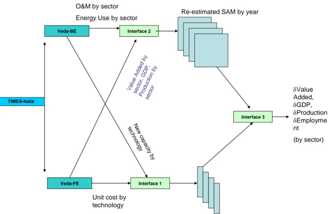
The principle of the linkage between TIMES model and SAM (or Energy-SAM) is depicted in Figure 1.
Figure 1 - Basic scheme of TIMES-SAM soft-linkage algorithm
The linkage consists in a series of interface, a VBA routines that perform the operations required to evaluate the economic impact of a energy scenario.
The first step involves a TIMES-Run. The results are a certain set of data like, for example: new installed capacity, cost and energy use for each TIMES Technology.
For details on interface 1, interface 2 [9-10]5 and interface 3 see a technical report by ENEA [14].
5
Among the main references see: [11-13].
TIMES-Italia Veda-BE Veda-FE New ca pa city by te ch no log y Interface 1 Unit cost by technology
Shock vectors by year
Interface 2 Va lue Ad ded by secto r, GDP , Pro du ction by secto r
Re-estimated SAM by year
Interface 3
O&M by sector Energy Use by sector
Value Added, GDP, Production Employme nt (by sector)
9
2. The application
This program, respect to the previous version6, is self-contained in a single interface hosted in a single Excel workbook. A main interface controls all the three routines, by executing the entire work flow or the three phases one by one. In the follows a detailed description of structure and operation of the main interface and the three routines is presented.
2.1 Modification of the Interface System
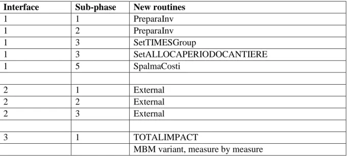
All the previous operations (performed by Interface 1, 2 and 3) have been collapsed in a unique structure following the scheme reported in table 1.
Interface Sub-phase New routines
1 1 PreparaInv 1 2 PreparaInv 1 3 SetTIMESGroup 1 3 SetALLOCAPERIODOCANTIERE 1 5 SpalmaCosti 2 1 External 2 2 External 2 3 External 3 1 TOTALIMPACT
MBM variant, measure by measure
Table 1 - Fitting table between the interfaces of the new program with the previous one.
Table 1 shows that the linkage operations, previously performed by three separate interfaces, are now managed by 7 routines hosted in the same program, contained in an excel file. The only exception is the balancing, still performed by the interface 2.
2.2 Main Interface Description
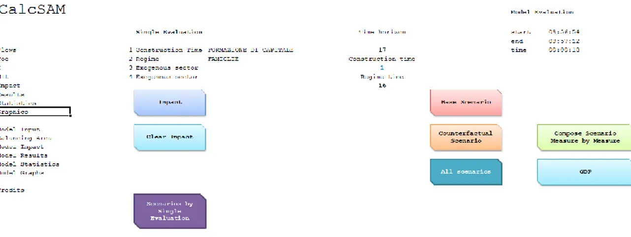
This routine is hosted in an .xlsm file that contain 33 sheets: the first is a control console that
6
10
reports the main contents, the key parameter that have to set to perform impact evaluation and the main routine commands.
Figure 2 show an excerpt of the control console of the interface.
Figure 2 - Main interface command console
Reading from left to right, and from up to down the control console reports:
the main sheets used:
Flows: the flows values in millions of euro;
Coe: the technical coefficients of the SAM;
I: the Identity Matrix;
Mlt: the multipliers;
Impact: the impact vector and the main output quantities;
Results: the Value Added, and the FTE labor units in output;
Stat: statistics on the previous output;
Graphics: some graphical elaborations of the output;
Model Input: the investment vectors used in the impact procedure, for the time horizon considered;
11
Model Impact: the impact results, reported in extended form (for all the economic activity sectors);
Model Results: the aggregate impact results, for 12 macro groups of economic and institutional activity sectors);
Model Statistics: the impact results, more aggregate than in Model Results, with some graphs;
Model Graphs: specific graphs extracted by elaboration of the output;
the main buttons:
Impact performs the impact for a single input vector;
Clear Impact erases results for the dedicated sheet (Model
Impact);
Scenarios by Single Evaluation perform the evaluation for a single scenario;
Base Scenario performs the evaluation for the Baseline scenario;
Counterfactual Scenario performs the evaluation for the Counterfactual
scenario;
All Scenarios perform the evaluation for a single scenario;
Compose Scenario Measure by Measure performs the evaluation by technology group;
GDP calculates GDP as a separate operation.
The "Single evaluation" section allows setting the exogenous sectors, respectively for the construction phase and for the regime phase. It also allows you to set up two other possible exogenous sectors, if necessary.
12
2.1 The linkage section
The link between technological models and the SAM is performed within a procedure of 5 step:
upload of investment vectors deriving from the technological model (INV sheet);
preparation of the vectors, namely allocation of the costs in the considered time period, on the basis of the specific construction time of each technology plant (INV sheet)
aggregation of investment costs for macro-groups of technologies (ST sheet);
allocation of the costs of each group in the SAM; this is done on the basis of allocation matrices (sheet %) that address the proportional distribution of the costs in the economic activity sectors (sheet Mea);
the same operations referred to in the previous point, are carried out for the counterfactual scenario (sheet MeaC);
aggregation of allocation data in the investment vector matrix in the SAM format (both in the SEv sheet, for a single scenario, than in the B&Cf sheet, in which multiple scenarios can be evaluated in sequence).
From this point, all the operations follows the normal scheme expected in the impact calculation, already described in [14].
13
2.2. Model evaluation sequence:
2.2.1. Uploading and preparing investment data
Scenario Process Set C_Time Process 2014 2015 ...
SC1 Set Code 1 Process code 1000 1000 ...
Table 2 - Investment data record structure
Table 2 reports the basic structure of investment data provided by the technical model. Each technology is characterized by a scenario name (like SC1), a process set, a construction time and a specific proper name. Every record of the dataset reports, year by year the amount of the investment required for each technology, for the entire time horizon considered.
The initial data are cumulative. To know how much actually spent on the construction of a plant, year by year, it is necessary to carry out a calculation step.
The value of each annual investment is divided by the time of construction, to obtain the real annual investment. This operation is performed for each year of the considered time horizon. The values obtained are added up gradually to each other, to arrive at the correct amount of annual investments by technology.
Stage Scenario ProcessSet C_ Time Process 2014 2015 2016 2017
SC 1 Set Code 2 SC1ELF005 0 1000 1000 0
Scenario ProcessSet C_ Time Process 2014 2015 2016 2017
SC 1 Set Code 2 SC1ELF005 500 500 1000 0
Scenario ProcessSet C_ Time Process 2014 2015 2016 2017
SC 1 Set Code 2 SC1ELF005 500 1000 = 500+500 500 0
Table 3 - An example of re-allocation of investment costs
Figure 3 illustrates an example of how the algorithm re-allocates costs.
At the first iteration, the fictitious SC1ELF005 technology has 1000 million euros of investments for the year 2015 and 2016. But in reality, the costs incurred are those related to
14
the end of the construction period. As this period is equal to 2 years, we can assume that the costs actually incurred were equal to 500 million euros for the year considered, and 500 for the previous year.
In the second step, proceeding by cell, we see that the 1000 million of 2016 are allocated half of the previous year. The procedure is repeated for the following year, so that, in the third step, the costs for 2016 amount to 1000 million euros (500 in 2016, and 500 from 2017). The entire procedure is replicated for each technology over the whole time horizon considered.
2.2.2. Creating Technology Groups to aggregate Investment costs
The second phase is straightforward and intuitive. The technologies are aggregated by homogeneous groups under some criteria (for example, all the electric ones that concern photovoltaics). Investments per group are obtained simply by adding the value of each technology to the others, year by year, as Figure 4 illustrates.
Scenario ProcessSet C_Time Process 2014 2015 2016 2017 2014 2015 2016 2017 SC 1 COM - PDC 2 SC1ELF005 0 1000 1000 0 ELF 0 3000 3000 0 SC 2 COM - PDC 3 SC1ELF006 0 1000 1000 0
SC 3 COM - PDC 4 SC1ELF007 0 1000 1000 0
Table 4 - An example of re-allocation of investment costs
2.2.3. Allocate Groups of Investment costs into SAM
This procedure is also direct and simple: the investment costs, year by year, group by group, are allocated among the sectors of economic activity of SAM according to predefined proportions.
2015 …
SCENARIO Group
SAM 2015
ELF 1000 … … …
Chemical products and artificial fibres 3% 30
Rubber and plastic products 0% 0
Other non metallic minerals 0% 0
15 Table 5 - Allocation of ELF sector in the SAM economic activity sectors
Looking at Figure 5, we have an example. If for the ELF technology group, in 2015 we have investments amounting to 1000 million euros, and for the chemical sector the proportion due to it is 3%, it will be allocated 30 million euros from the total.
2.2.4. Building the final matrix of investment vector
Once the costs are allocated within the SAM business sectors, the costs are calculated, year by year, by group type.
In this way, a total matrix is obtained that represents the investment vectors with which to impact the SAM year by year. From this point on, the impact calculation operations continue as per standard literature.
The program also offers the possibility of composing investment vectors, cumulated and by group of technologies.
In this way, it is possible to consider the effect of every single measure concerning a specific group of technologies.
From this point, all the operations follows the normal scheme expected in the impact calculation, already described in [14].
16
3. Output
What follows reports a brief and not exhaustive list of the main statistical output available from the application.
3.1 GDP dynamics over time, for one or more scenario and their Counterfactuals (% of GDP)
3.2 Value Added over time of a specific scenario (millions of euro) for a selected period/macrosectors 0% 1% 2% 3% 4% 5% 6% 2016 2017 2018 2019 2020 2021 2022 2023 2024 2025 2026 2027 2028 2029 2030 Scenario Counterfactual 0,0 10,0 20,0 30,0 40,0 50,0 60,0 70,0 80,0 90,0 2020 2021 2022 2023 2024 2025 2026 2027 2028 2029 2030 INDUSTRY SERVICES
17 3.3 Value Added over time of a specific scenario (millions of euro) for a selected period/2 or more sectors
3.4 Value Added over time of a net scenario (Baseline - Counterfactual) (millions of euro) for a selected period/macrosectors € - € 5 € 10 € 15 € 20 € 25 € 30 € 35 € 40 2020 2021 2022 2023 2024 2025 2026 2027 2028 2029 2030 Forestry Fishing 0,0 5,0 10,0 15,0 20,0 25,0 30,0 35,0 40,0 45,0 2020 2021 2022 2023 2024 2025 2026 2027 2028 2029 2030 INDUSTRY SERVICES
18
3.5 Value Added over time of a net scenario (Baseline - Counterfactual) (millions of euro) for a selected period/2 or more sectors
3.6 FTE Labor Units over time of a specific scenario (millions of euro) for a selected period/macrosectors (thousand units)
-€ 20 € - € 20 € 40 € 60 € 80 € 100 € 120 2020 2021 2022 2023 2024 2025 2026 2027 2028 2029 2030 Forestry Fishing 0,0 10,0 20,0 30,0 40,0 50,0 60,0 70,0 80,0 90,0 2020 2021 2022 2023 2024 2025 2026 2027 2028 2029 2030 INDUSTRY SERVICES
19 3.7 FTE Labor Units over time of a specific scenario (millions of euro) for a selected period/macrosectors (thousand units)
3.8 FTE Labor Units over time of a specific scenario (millions of euro) for a selected period/macrosectors (thousand units)
0 20 40 60 80 100 120 140 2020 2021 2022 2023 2024 2025 2026 2027 2028 2029 2030 Forestry Fishing 0,0 5,0 10,0 15,0 20,0 25,0 30,0 35,0 40,0 45,0 2020 2021 2022 2023 2024 2025 2026 2027 2028 2029 2030 INDUSTRY SERVICES
20
3.9 FTE Labor Units over time of a specific scenario for a selected period/macrosectors (thousand units)
3.10 Value Added for a single technology group over time for a macrosectors cumulated value for years 2020-2030 (millions of euro)
-20 0 20 40 60 80 100 120 2020 2021 2022 2023 2024 2025 2026 2027 2028 2029 2030 Forestry Fishing 11,74 4,15 8,80 3,71 Baseline Counterfactual Industry Services
21 3.11 FTE Labor Units for a single technology group over time for a macrosectors for a net scenario (Baseline - Counterfactual) (cumulated value for years 2020-2030) (thousand units)
3.12 Energy policy - Breakdown of investment by group of technology among SAM economic activity macro-sectors (Case: ELE PV, Baseline scenario, 2016)
42,27 -0,15 Baseline Industry Services 87% 12% 1% Industry Services Other
22
4. A Case Study
Climate change is strongly related to energy security and economic growth as, for example, the dilemma between economic growth and climate change mitigation well shows [15-16]: so, in the field of support of energy-environmental policy making, an interdisciplinary approach both at public level [17-18] and at business level is required to address properly that challenges [19], as well as the development of new methods appears crucial [20].
The purpose of this work is to outline a new methodology in comparing different energy policy options. A Cost-Effectiveness Analysis (C-E A) was performed for two different energy scenarios for Italy, in the period 2016-2030. The C-E A was implemented using a Markov model, combining two types of input: the output of a technical-economic model (TIMES model) [21-24] and the output of an economic model (SAM).
In particular, two different scenarios are compared: a Baseline scenario and a Policy scenario, being the Policy scenario designed to give a more significant answer to climate change than the Baseline scenario.
Basically, some key energy data are used as input for macroeconomic analysis, to analyze the impacts on the main economic variables (like GDP) of two different evolutions of the energy system and, above all, of the decarbonisation policies.
The results produced by the two models, TIMES and SAM, were then used in a cost-effectiveness analysis in which uncertainty was taken into account. In particular, uncertainty was considered relative to the GDP parameter, in the third phase of the analysis (the C-E A).
In this work we did not consider feedback between the TIMES and SAM models, but they were made coherent with each other through a SAM updating procedure developed by some of the authors [25-27], which will be discussed in the methodology section.
The work is structured as follows: the methodological part give some quick note on the three tools used, then reports some notes about the models and their linkage and about some key assumptions.
The results section reports:
• for TIMES-Italy model: the investments aggregated by type of technology and the CO2 emissions for the considered time-horizon, expressed in billions of euro. The parameters and key drivers used to implement the scenarios are also shown;
23 • for SAM, the impact on GDP of each scenario and the impact on FTE labor units. The calculations of impact on the Value Added have been omitted due to an arbitrary choice operated handling the great amount of data generated;
• for the Markov model, we report the result of the cost-effectiveness analysis, expressed in terms of billions of euro on millions of tons of avoided CO2.
The cost-effectiveness analysis and the uncertainty were managed through the use of a Markov model [28-30]. The cost was represented by the investments and the effectiveness by and CO2 emissions in order to perform the C-E A.
The above mentioned choice was made due to the large amount of data produced by the first two models leaded to a drastic simplification of the last step of the analysis.
The concluding part includes some considerations about the methodology, the results and the policy implications.
4.1 Methodology
What follows reports some basic information on the main tool used in this work. 4.1.1 TIMES models
The Integrated MARKAL-EFOM System (TIMES) model generator was developed by IEA-ETSAP (Energy Technology Systems Analysis Program) combines two approaches to modeling energy: the technical engineering one, and the economic one. Quoting IEA: "TIMES is a technology rich, bottom-up model generator, based on linear-programming to produce a least-cost energy system, optimized according to a number of user constraints, over medium to long-term time horizons" [31].
4.1.2. Social Accounting Matrix (SAM)
A Social Accounting Matrix (SAM) reports all the economic transactions that take place within an economy geographically identified as a matrix representation of the National Accounts in a period of time (year).
Technically, is a square matrix, since economic players considered appear as buyers (column) and as sellers (rows). Columns represent buyers (expenditures) and rows represent sellers (receipts).
24
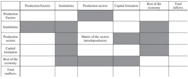
The SAM is read from column to row, ensuring that each entry from its column heading, going to the row heading. The sum of columns and rows must be equal, to ensure accounting consistency. Figure 4 reports a graphical illustration of a SAM for a basic open economy [32].
Figure 4 - Basic scheme of a Social Accounting Matrix.
SAM's were originally developed by Stone in the context of “Cambridge Growth Project” in 1962 [25].
SAMs can be easily extended to include other flows in the economy, simply by adding more columns and rows: furthermore, the inverse of this operation (disaggregation) is also possible [33] and was performed by some of the authors to better represent the energy sector [34].
SAMs is also strongly connected with the Computable general equilibrium (CGE) Models and various types of empirical multiplier models.
An important note is the following: for each scenario, we consider both the impact of the scenario itself and the so-called "counterfactual". In practice, the counterfactual scenario is calculated by using the same amount of investments expected for each scenario, using a different proportional distribution between the economic activity sectors.
In practice: for each scenario, it is necessary to know how the investments will be allocated among the sectors, an operation that must be done each time in a specific way. In the counterfactual scenario, instead, the same investments are allocated among the sectors according to a "business as usual" distribution.
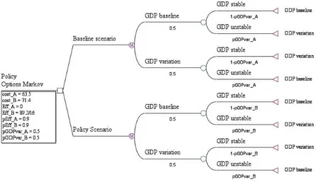
25 2.3. Markov modeling for Cost-Effectiveness Analysis
Variables Description Units GDP stable GDP unstable
Cost_A
Total annual cost of Policy A
billions of euro 63.5 63.5 - pGDPVar*16 Cost_B Total annual cost of Policy A billions of euro 71.4 71.4 - pGDPVar*80
Eff_A Effectiveness of Policy A
mln of tons of CO2 avoided
0 0
Eff_B Effectiveness of Policy B mln of tons of CO2 avoided 89,2/15 89,2/15
pEff_A Probability of success of Policy A % 90% 90%
pEff_A Probability of success of Policy B % 90% 90%
pGDPvar_A Probability of GDP variation for Policy A % 0% 50%
pGDPvar_B Probability of GDP variation for Policy B % 0% 50%
Table 6 - Input of Cost-Effectiveness Analysis
Table 6 reports the input for Cost-Effectiveness Analysis for each policy considered, namely: the costs (expressed as the annual investment cost); the effectiveness (expressed in Mton of CO2 avoided); "the probability of success" of the policy (the probability of achieve
the results, in terms of emissions reduction) and, finally, the probability of a GDP variation (fixed to an arbitrary value of 50% for both the policies). In the sample analyzes carried out, policy A represents the decarbonisation options of the Policy scenario, while policy B represents the Baseline scenario.
The cost-effectiveness analysis was made as follows. Only the technology investment cost was used to represent the annual cost of the policies (Remember that we only consider the impact of policy on the construction phase of interventions or technologies, but we do not consider the effect on the regime phase). The effectiveness was calculated in terms of millions of tons of CO2 avoided.
Furthermore, the costs were considered in two different ways. In the first case, we have taken into account only the investment costs of each policy. In the second case, we considered a "net cost" measure, obtained by subtracting from investment costs, the positive change in
26
GDP that these investments caused. The correction is calculated as the product of the probability of variation of GDP for a numerical value, equal to 16 in the case of Policy A, and to 80 in the case of Policy B. These values, expressed in millions of euro, represent the gain in terms of GDP related to the economic impacts of the scenarios considered. For example, the impact of Policy B, in terms of GDP, is equivalent to an average annual increase of around € 80 billion. Such a value must be multiplied to the fixed probability of GDP variation to obtain the correct value of this "compensation". With regard to Policy A, which corresponds to the Baseline scenario, the relative economic impact leads to an increase in GDP of around € 16 billion a year. The rational of this calculation is to provide a more realistic measure of the cost of each policy.
Indeed, the calculation should be likely very more complex: total real costs and income (value added, taxation, ...) were not considered in our simplification, for example.
The probability of changes in GDP impact has been arbitrarily set at 50%, for both scenarios: a rather unlikely hypothesis, made even for the sake of simplicity (indeed, it would be necessary to be able to evaluate the probability of growth for the two scenarios that is largely outside from the scope of this work).
Furthermore, a "probability of success" has been given to the policies implemented, using an arbitrary value, 90% (as it would be a very complex matter, or a mission impossible, to attribute to them a "real" value). Such a high number corresponds to a strong confidence in the result of investments, in terms of effectiveness about climate change mitigation. About the costs, they correspond to the arithmetic average of the sum of investments in the period considered (2016-2030).
The performed analysis represents just a simplification made in a purely methodological context: nevertheless, it shows the potential of an interdisciplinary analysis in which it is possible to take into account uncertainty.
Figure 5a and 5b shows the decision tree corresponding to the used Markov model in the two case studies considered (with or without the compensation from positive impact of the policies on GDP).
27 Figure 5a. Markov model used in simulation without correction cost via GDP variation.
Figure 5b. Markov model used in simulation with correction cost via GDP variation.
4.1.3. Linking model, assumptions and simplifications
About the link between TIMES model and SAM, the analysis was based on ECN study [35] and on a related methodology developed by the authors [36], to which we refer for any methodological insights. The linkage between TIMES, SAM and the Markov model is established through two interfaces. The first interface transforms and re-allocates energy costs associated with TIMES technologies to comply with the structure of the SAM. The second interface uses the results from the SAM as input for a Markov model implemented to perform the dynamic cost-effectiveness analysis cited in section 2.4.
28
The analysis starts with the TIMES model. The results of this model consist of information on, among others, new installed capacity, cost and energy use for each TIMES Technology. The output of TIMES is passed, through interface 1 to SAM: mainly, the investment costs provided by TIMES are allocated into the economic activity sector of the Social Accounting Matrix. Finally, the investment cost and CO2 emissions from TIMES, and the GDP variation from SAM are then passed on to interface 2 to feed the Markov model and make the Cost-Effectiveness Analysis.
Two different energy policies were compared, one of which was characterized by a higher level of investment in renewable technologies (the Policy scenario that is more "aggressive" in the climate change mitigation). The time-horizon was set from 2016 to 2030.
A first clarification to be made concerns the type of impact calculated. We have considered, for the sake of simplification, only the so-called "investment" period, and not the "regime" period.
Therefore, the full effects in the "regime" phase of the investments made are not considered. This choice was made since the scope of our work was just to outline the potential of the used methodology rather than to analyze a real case study. As we said before, TIMES and SAM have been "harmonized". This means that the expected trend for the GDP used as input for the TIMES model was "imposed" on the SAM matrix using a specific balancing procedure. The matrix is balanced with a variant of the well-known RAS method. In practice, the GDP dynamics used in the TIMES model can be made consistent with the evolution of SAM's technical coefficients during the period considered. This work was performed using a matrix balancing procedure designed to update its technical coefficients over time. This type of operation is in particular carried out by means adding constrains in the balancing of the SAM, namely, keeping some coefficients of the SAM "blocked" at a certain level. All the technical details of these operations are reported in a previous works by some of the authors [37].
Finally, uncertainty is referred to GDP dynamics, depending on some considered energy policy hypotheses, which will be illustrated below.
4.2 Results
Looking at the detailed results we can start from a compact representation of the investments expected in the two scenarios produced by TIMES model. The detail of the technologies considered in the TIMES model is considerable: over 500 types of different
29 technologies was considered. To make the data representation easier, the aforementioned technologies have been grouped into five macro-groups following an internal classification of the TIMES model technology:
electrical technologies (Electrical Tech Group) manufacturing technologies (Industrial Tech Group)
technologies for the residential sector (Residential Tech Group) transport technologies (Transport Tech Group)
technologies for the commercial sector. (Commercial Tech Group)
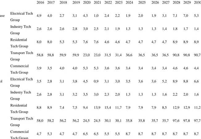
Table 7 and Figure 6 shows the amount of the investment expected in the two scenarios considered, expressed in billions of euro. We can see that Policy scenario is characterized by a considerable increase in the level of the investment (about 121 billions of euros higher than Baseline, +10,4% in terms of percentage difference).
2016 2017 2018 2019 2020 2021 2022 2023 2024 2025 2026 2027 2028 2029 2030
Base Electrical Tech Group 4,9 4,0 2,7 3,1 4,3 1,0 2,4 2,2 1,9 2,0 1,9 3,1 7,1 7,0 5,3 Industry Tech Group 2,6 2,6 2,6 2,8 3,0 2,5 2,1 1,9 1,3 1,3 1,3 1,4 1,8 1,7 1,4 Residential Tech Group 8,0 8,0 5,3 5,3 7,6 7,6 4,6 4,6 4,7 4,7 4,7 4,7 8,9 8,9 8,9 Transport Tech Group 58,8 58,8 59,9 59,9 23,0 23,0 31,5 31,4 36,6 36,5 36,5 36,5 90,8 90,8 90,7 Commercial Tech Group 3,9 3,5 4,0 4,0 5,3 5,3 3,6 3,6 3,4 3,4 3,4 3,4 4,6 4,6 4,4
Pol Electrical Tech Group 3,5 2,8 3,1 3,8 4,5 0,9 3,1 3,0 3,5 3,6 3,6 5,2 8,9 8,8 6,6 Industry Tech Group 2,6 2,8 3,1 3,2 3,5 3,0 2,3 2,0 1,3 1,3 1,3 1,6 2,2 2,0 1,6 Residential Tech Group 8,8 8,9 7,4 7,5 9,4 13,9 15,4 11,7 7,9 7,9 7,9 8,5 12,9 12,9 11,2 Transport Tech Group 58,0 58,2 56,2 56,2 24,5 24,5 30,1 30,1 35,8 35,8 35,7 35,7 97,6 97,8 97,7 Commercial Tech Group 4,7 5,3 4,7 4,7 6,5 6,5 5,5 5,5 8,7 8,7 8,7 8,7 8,7 8,7 8,7
Table 7 - Breakdown of total expected investment for Baseline scenario and Policy scenario by group of technology (data in millions of euro)
30
Figure 6 - Total expected investment for Baseline and Policy scenario's (data in billions of euro).
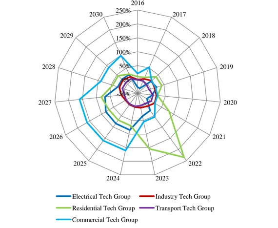
Figure 7- Breakdown of percentage investment variation by group of technology for Baseline scenario and Policy scenario from 2016 to 2030 (data in %).
0,0 20,0 40,0 60,0 80,0 100,0 120,0 140,0 160,0 2014 2016 2018 2020 2022 2024 2026 2028 2030 2032 In v est m en t ex p ec te d ( b il li o n s o f eu ro s) Years
Baseline scenario Policy scenario
-50% 0% 50% 100% 150% 200% 250% 2016 2017 2018 2019 2020 2021 2022 2023 2024 2025 2026 2027 2028 2029 2030
Electrical Tech Group Industry Tech Group Residential Tech Group Transport Tech Group Commercial Tech Group
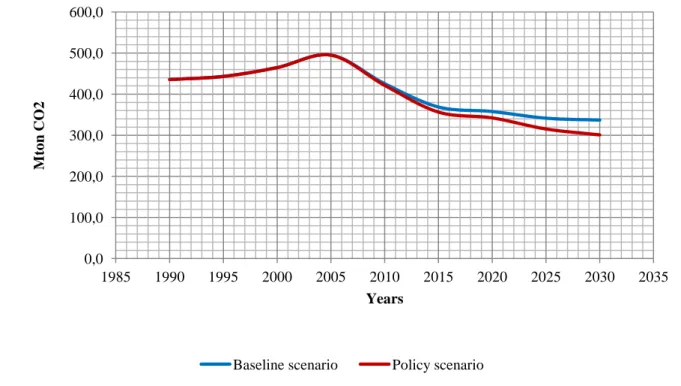
31 Figure 7 shows the percentage change in the level of investment between the Baseline scenario and the Policy scenario, by groups of technologies. Total investments in the Policy scenario are 37% higher than the Baseline scenario. The most significant differences are found for the Residential Tech Group (+ 67% for the Policy scenario compared to the Baseline scenario) and Commercial (+ 79%): the Transport Tech Group remains substantially stable. Regarding the emissions trend, Figure 5 reports the emission trend emissions linked to the Baseline scenario and to Policy scenario provided by TIMES model: the Policy scenario allows a decreasing in CO2 emissions equal to -19.4% in the years from 2016 to 2030 respect to the Baseline.
Figure 8 - CO2 emission (data in millions of tons of CO2).
Moving to the SAM results, let's start by considering the effects on GDP impacts of the arbitrarily fixed variations mentioned in the Methodology section. Figure 8 reports the absolute variation (expressed in millions of euro) of GDP due to an arbitrary change of -0.2%. The change considered (-0.2%) is more significant in the Policy scenario (where it produces average variability effects on GDP of the order of 0.11%) compared to the Baseline scenario (0.03%): regarding the counterfactual scenarios the numbers turn in, respectively, 0.02% against 0.05). All the results, calculated as a percentage, are subsequently converted into euro by multiplication to Italian GDP of year 2018.
0,0 100,0 200,0 300,0 400,0 500,0 600,0 1985 1990 1995 2000 2005 2010 2015 2020 2025 2030 2035 M to n CO 2 Years
32
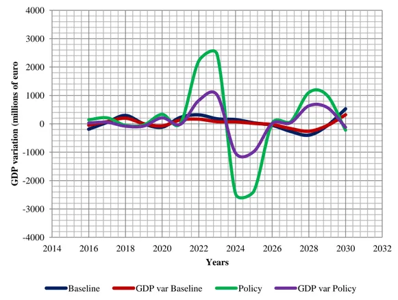
Figure 9 - Sensitivity analysis of GDP trend by arbitrary GDP variation of 0.2%.
Figure 9 shows a little more complex elaboration: the GDP variations (in %) produced by the Policy scenario minus the variations produced by the Baseline scenario.
For each scenario, the annual variation of the GDP produced is calculated: subsequently, the GDP changes produced by the Baseline scenario are detracted by the ones produced by the Policy scenario.
Figure 10 illustrates the differences in GDP growth between the two scenarios, Policy and Baseline, also calculated for the respective counterfactual scenarios. Finally, the calculated percentage changes have been converted into absolute values (in euro) using as a reference value the Italian GDP in 2018.
The differences between the two scenarios are remarkable, with an average annual growth for the Policy scenario of 2.98% against 2.67% of Baseline scenario (1.62% against 1.48% for the respective Counterfactuals).
-4000 -3000 -2000 -1000 0 1000 2000 3000 4000 2014 2016 2018 2020 2022 2024 2026 2028 2030 2032 G DP v a ria tio n (m il li o n s o f eu ro Years
33 Figure 10 - Changes in GDP between Baseline scenario and Policy scenario and between their counterfactual (data in billions of euro).
About the FTE Labor Units, Table 8 shows the results of each scenario, near by the respective counterfactual and the net impact (scenario - counterfactual). The table shows the average values in thousands of units per year. A more detailed look reveals that major increase regards Industry, Construction, Services and Transport sector.
Table 8 - Breakdown of Average FTE Labor Unit per year for Baseline and Policy
scenario's by macro-sectors of economic activity (thousands of FTE Unit).
Baseline Policy
Scenario Counterfactual Net Scenario Counterfactual Net
Agriculture 6,27 3,95 2,32 6,49 4,12 2,37
Mining and Quarrying 31,72 15,82 15,90 34,44 17,32 17,12
Industry 806,02 402,87 403,15 860,09 442,53 417,56
Energy and Water 60,28 17,82 42,47 63,55 19,29 44,26
Construction 34,89 275,67 -240,78 55,23 304,33 -249,10 Services 715,33 318,46 396,86 772,61 345,01 427,60 Transport 120,71 46,91 73,80 130,41 51,09 79,32 Government 89,25 126,40 -37,15 98,75 138,14 -39,38 -4,0 -2,0 0,0 2,0 4,0 6,0 8,0 10,0 12,0 14,0 16,0 18,0 2014 2016 2018 2020 2022 2024 2026 2028 2030 2032 G DP v a ria tio n (m il li o n s o f eu ro s) Years
34
Figure 11 - Average FTE labor units per year resulted by macroeconomic impact calculated for net Baseline and net Policy Scenario (net = Scenario - Counterfactual) (thousands of FTE Unit).
4.2.1 Cost Effectiveness Analysis
The results of the cost-effectiveness analysis are eloquent. The Policy scenario is confirmed as the only effective, with a cost slightly higher than the Baseline. Regarding the measurement of effectiveness, we only took into account the best scenario. Given X the difference between the two scenarios, we have set the effectiveness of the worst case scenario to 0, and assigned X to the other. Since effectiveness is measured in terms of avoided emissions, it follows that this measure is equal to 0 for the Baseline, by definition, and is positive for the Policy, which is automatically winning since it is characterized by a lower level of emissions than its counterpart.
Clearly, this choice is the result of an arbitrary convention. The logical sense of the aforementioned choice is to be found in the state of emergency posed by the ongoing climate change. In any case, it is easy to verify that, even considering the effectiveness of the Baseline scenario, the results of the C-E Analysis would be equivalent.
About the costs, in the time horizon considered, the cumulative cost of the two policies is equal to 920 billion euro for the Baseline scenario and 1035 billion euro for the Policy one.
403,15 -240,78 396,86 73,80 417,56 -249,10 427,60 79,32 -300,00 -200,00 -100,00 0,00 100,00 200,00 300,00 400,00 500,00
Industry Construction Services Transport
35 We observe that these values are lower than those of the investment data produced by the TIMES model, since in the analysis they were subject to probabilistic fluctuations (in the simulation, the scenario data have to passed through the so called Markov probability transition matrix).
Considering the net benefits, calculated as the GDP change on the investment costs, the situation is completely reversed: the cumulative cost of the two policies is equal to 804 billion euro for the Baseline scenario and 455 billion euro for the Policy one. In this case, the Baseline scenario is, as it is usually called, "strictly dominated" by the Policy scenario.
Figure 12a - Cost-effectiveness analysis results in comparison of Baseline and Policy scenario (costs data in billions of euro, effectiveness data in Mt of CO2 avoided) without net effects via GDP variation.
36
Figure 12b - Cost-effectiveness analysis results in comparison of Baseline scenario and Policy scenario (costs data in billions of euro, effectiveness data in Mt of CO2 avoided) with cost correction via GDP variation.
4.3 Conclusions
In this work, a complex methodology in energy and economic analysis has been used in an interdisciplinary context in order to compare two alternative energy policies. In particular, two scenarios of the energy system provided by TIMES model for Italy were compared: a Baseline scenario, characterized from a certain amount of investment to climate change mitigation and a Policy scenario, more effective than the Baseline. The selected time horizon covers the years from 2016 to 2030.
The comparison between alternative energy scenarios is a well consolidated research area [38-40]: in this work, the authors have brought some methodological results and insights developed supporting to the public decision-making in Italy (namely, the elaboration of National Energy Strategy).
37 The macroeconomic impact (GDP, FTE Labor Units) was resulted by the link between the TIMES Italia model and the Social Accounting Matrix for Italy. The output of TIMES model and SAM was then used in a final step, to perform a cost-effectiveness analysis implemented through a Markov model.
The cost was represented, for each Policy, by the investments made: the effectiveness, by the savings in CO2 emissions produced.
The results obtained show that the most effective policy is also, not surprisingly, more expensive. However, a net cost measure, obtained by subtracting from these costs the impact on GDP of the policies, results in a clear reversal of the ranking, making the most effective policy as the most convenient one.
Although limited, this analysis provided very useful hints about the possibilities of extending the interactions between energy system models and economic models. Cost-effectiveness analysis was applied to the comparison between energy scenarios in different contexts [41-42]: in our case we wanted to apply it to two well-known model types to show some of the potential of this kind of analysis. In particular, the C-E A applied to the TIMES model and to SAM, could be applied to a large amount of data (both energetic and economic), combined with the emissions data of the each scenario.
It must be remember that, ideally, an evaluation system should include a real feedback between the results of the two models, mainly through the macroeconomic variables like the GDP. The performed analysis is to be considered as a sort of first order evaluation, aimed at indicating a research direction, rather than providing operative tools, just ready to address current issues.
Furthermore, there are versions of the TIMES model able to take into account uncertainty, as there are versions of macroeconomic models able to do the same (about this point, the authors have developed a methods about the updating of the technical coefficients of SAM).
Creating integration tools for the purpose of integrating the aforementioned models is certainly an interesting ongoing research area. Finally, the cost-effectiveness analysis and the Markov models, provides consolidated and flexible analytical tools to take into account uncertainty in the main variables of the used model
38
Bibliography
1. Gaeta, M., & Baldissara, B. (2011). Il modello energetico TIMES-Italia: struttura e dati. Roma: ENEA.
2. Marco Rao, Umberto Ciorba, Giovanni Trovato, Carmela Notaro, Cataldo Ferrarese: Estimating an Energy-Social Accounting Matrix for Italy. The New Generation of Computable General Equilibrium Models, 05/2018: pages 65-83; , ISBN: 978-3-319-58532-1, DOI:10.1007/978-3-319-58533-8_4
3. Loulou, R., Goldstein, G., & Noble, K. (2004). Documentation for the MARKAL Family of Models. Paris: IEA.
4. Loulou, R., Remne, U., Kanudia, A., Lehtila, A., & Goldstein, G. (2005). PART I. In R.
5. U.N. (1968). A System of National Accounts. New York: U.N.
6. U.N. (s.d.). Tratto il giorno February 2, 2014 da System of National Accounts 2008: http://synagonism.net/standard/economy/un.sna.2008.html
7. Miller, R., & Blair, P. D. (2009). Input-Output Analysis: Foundations and Extensions. New York: Cambridge University Press
8. Klaassen, M., Vos, D., Seebregts, A., Kram, T., Kruitwagen, S., Huiberts, R., et al. (1999). Markal-IO : Linking an input-output model with MARKAL. Bilthoven, The Netherlands: NOP Commission.
9. Rao, M., & Tommasino, M. C. (2015). Roma: ENEA.
10. Rao, M., & Tommasino, M. C. (2014). Updating technical coefficients of an input-output matrix with RAS - the TRIOBal software. Roma: ENEA.
11. Lahr, M., & De Mesnard, L. (2004). Biproportional techniques in input-output analysis: table updating and structural analysis. Economic Systems Research , 115-134.
12. Gilchrist, D. A., & St Louis, L. V. (1999). Completing Input-Output Tables using Partial Information, with an Application to Canadian Data. Economic Systems Research , 185-194.
13. Szyrmer, J. (1989). Trade-Off between Error and Information in the RAS Procedure. In K. P. R. Miller, Frontiers of Input-Output Analysis (p. 258-277). New York: Oxford University Press.
39 14. Rao, M., Ciorba, U., Tommasino,M.C., Gaeta, M. (2015) A software application for TIMES-SAM linkage: A VBA program to connect energy and macroeconomics models. Roma: ENEA.
15. Tol, R.S.J., The Economic Impacts of Climate Change. Review of Environmental Economics and Policy, 2018; 12, 1: 4–25. DOI:10.1093/reep/rex027
16. Rezai, A., Taylor, L., Foley D., Economic Growth, Income Distribution, and Climate Change. Ecological Economics, 2018; 146: 164-172. DOI: 10.1016/j.ecolecon.2017.10.020
17. Bertrand N., Jones L., Hasler B., Omodei-Zorini L., Petit S., Contini C. (2008) Limits and targets for a regional sustainability assessment: an interdisciplinary exploration of the threshold concept. In: Helming K., Pérez-Soba M., Tabbush P. (eds) Sustainability Impact Assessment of Land Use Changes. Springer, Berlin, Heidelberg
18. Murray, A., Skene, K., Haynes, K., The Circular Economy: An Interdisciplinary Exploration of the Concept and Application in a Global Context, Journal of Business Ethics, 2017; 140: 369-380. DOI: 10.1007/s10551-015-2693-2
19. Paul, A., Lang, W. B., Baumgartner, R. J., A multilevel approach for assessing business strategies on climate change, Journal of Cleaner Production, 2017; 160: 50-70. DOI: 10.1016/j.jclepro.2017.04.030
20. Schütte, S., Gemenne, F., Zaman, M., Flahault, A., Depoux, A. , Connecting planetary health, climate change, and migration, The Lancet Planetary Health, 2018; 160: e58-e59. DOI: 10.1016/S2542-5196(18)30004-4
21. Seebregts A.J., Goldstein G.A., Smekens K. (2002) Energy/Environmental Modeling with the MARKAL Family of Models. In: Chamoni P., Leisten R., Martin A., Minnemann J., Stadtler H. (eds) Operations Research Proceedings 2001. Operations Research Proceedings 2001 (Selected Papers of the International Conference on Operations Research (OR 2001) Duisburg, September 3–5, 2001), vol 2001. Springer, Berlin, Heidelberg
22. Loulou, R., Goldstein, G., & Noble, K. (2004). Documentation for the MARKAL Family of Models. Paris: IEA.
23. Loulou, R., Remne, U., Kanudia, A., Lehtila, A., & Goldstein, G. (2005). PART I. In R. Loulou, U. Remne, A. Kanudia, A. Lehtila, & G. Goldstein, Documentation for the TIMES Model (p. 1-78). Paris: IEA.
40
24. Gaeta, M., & Baldissara, B. (2011). Il modello energetico TIMES-Italia: struttura e dati. Roma: ENEA RT-2011-09.
25. Stone, R. and Brown, A., 1962, A computable model of economic growth, University of Cambridge. Dept. of Applied Economics Chapman & Hall, London 26. Miller, R., & Blair, P. D. (2009). Input-Output Analysis: Foundations and
Extensions. New York: Cambridge University Press.
27. U.N. (1968). A System of National Accounts. New York: U.N.
28. Alagoz, O., Hsu, H., Schaefer, A.J., 2009 Markov Decision Processes: A Tool for Sequential Decision Making under Uncertainty. Medical Decision Making, DOI:10.1177/0272989X09353194
29. Lund, Robert B. "Markov Processes for Stochastic Modeling." Journal of the American Statistical Association, vol. 93, no. 442, 1998, p. 842. Academic OneFile, Accessed 30 Nov. 2018.
30. Charfeddine, L, 2017. The impact of energy consumption and economic development on Ecological Footprint and CO2 emissions: Evidence from a Markov Switching Equilibrium Correction Model. Energy Economics, DOI: 10.1016/j.eneco.2017.05.009
31. International Energy Agency 2018 - ETSAP -
https://iea-etsap.org/index.php/etsap-tools/model-generators/times
32. Scandizzo P.L., Ferrarese C., and Vezzani A., 2010, La Matrice di Contabilità Sociale: una nuova metodologia di stima, in Il Risparmio Review
33. Wolsky, A.M., 1984, Disaggregating Input-Output models, in The Review of Economics and Statistics, Vol. 66, No. 2 (May, 1984), pp. 283-291, The MIT Press 34. Rao M., Ciorba U., Trovato G., Notaro C., Ferrarese C. (2018) Estimating an Energy-Social Accounting Matrix for Italy. In: Perali F., Scandizzo P. (eds) The New Generation of Computable General Equilibrium Models. Springer, Cham 35. Klaassen, M.A.W.; Vos, D.; Seebregts, A.; Kram, T.; Kruitwagen, S.; Huiberts, R.;
Ierland, E.C. van. Markal-IO : Linking an input-output model with MARKAL (1999). Bilthoven, The Netherlands: NOP Commission
36. Rao, M., Tommasino, M. C., Ciorba, U, Gaeta, M. (2015). A SOFTWARE APPLICATION FOR TIMES-SAM LINKAGE - A VBA program to connect energy and macroeconomic models. Roma: ENEA
37. Rao, M., & Tommasino, M. C. (2014). Updating technical coefficients of an input-output matrix with RAS - the TRIOBal software. Roma: ENEA
41 38. Barton, J., Davies, L., Dooley, B., Foxon, T.J., Galloway, S., Hammonde, G.P, O’Gradye, A., Robertson, E. Thomson, M. 2017. Transition pathways for a UK low-carbon electricity system: Comparing scenarios and technology implications. Renewable and Sustainable Energy Reviews, Volume 82, Part 3, February 2018, Pages 2779-2790
39. Alvarenga, A., Seixasa, J., Rodrigues, S. Long-term energy scenarios: Bridging the gap between socio-economic storylines and energy modeling. 2015. Technological Forecasting and Social Change. Volume 91, February 2015, Pages 161-178
40. Connolly, D., Lund, H., Mathiesen, V. Smart Energy Europe: The technical and economic impact of one potential 100% renewable energy scenario for the European Union. 2016. Renewable and Sustainable Energy Reviews Volume 60, July 2016, Pages 1634-1653
41. Cantore, N., Nussbaumer, P., Wei, M., Kammen, D.M. Promoting renewable energy and energy efficiency in Africa: a framework to evaluate employment generation and cost effectiveness. 2017. Environmental Research Letters, Volume 12, Number 3
42. Roth, M.B., Jaramilla, P. Going nuclear for climate mitigation: An analysis of the cost effectiveness of preserving existing U.S. nuclear power plants as a carbon avoidance strategy. 2017. Energy. Volume 131, 15 July 2017, Pages 67-77
42
Appendix A – Routines list by name, description, number of rows
Name Description rows
1 AggrMeas Aggregate results in B&Cf sheet 50
2 ClearSingleEvaluation 'This routine run the Interface 1 46 3 ClearSingleEvaluationC 'This routine run the Interface 2 46
4 CoeCut cut the exogenous sectors from coe matrix 91
5 CoeCutC Idem as above for the Counterfactual 91
6 ComposeScenario Calculate mea by mea the B scenario and its C 17 7 CountAndCut cut the ROW and CF sectors from Mlt matrix 41
8 CountAndCutC Idem as above for the Counterfactual 41
9 ExoCut cut the exogenous sectors from Mlt matrix 40
10 ExoCutC Idem as above for the Counterfactual 40
11 Impact Performs a single impact 18
12 ImpactC Idem as above for the Counterfactual 18
13 MakeCoe Create the coefficient matrix (coe) 62
14 MakeCoeC Idem as above for the Counterfactual 62
15 MakeIA Multiplicates I for Coe 49
16 MakeIAC Idem as above for the Counterfactual 49
17 MakeID create the Identity Matrix (I) 53
18 MakeIDC Idem as above for the Counterfactual 53
19 MBM Calculate impact by technology group 79
20 Measures Allocate measure in SAM by technology
group 59
21 MeasuresC Idem as above for the Counterfactual 59
22 Mlt create the multipliers (Mlt) from flows 239
23 MltC Idem as above for the Counterfactual 239
24 MtGen create (Mlt) in a general way 43
25 MtGenC Idem as above for the Counterfactual 43
26 PreparaInv Prepare Investment Vectors 6
27 Scenarios Calculates Base and Counterfactual scenario 148
28 ScenarioSEv Same as above, for a single scenario 148
29 SetALLOCAPERIODOCANTIERE Associate constr time to technology groups 146 30 SetTIMESGroup Allocate investment by technology groups 154 31 SpalmaCosti Re-allocate investment using a constr time 80
32 TOTALIMPACT Calculate impact in terms of Value Added 408
33 TOTALIMPACTCF Idem as above for the Counterfactual 408
34 TOTALIMPACTPIL Calculate PIL for Baseline Scenario 45
35 TOTALIMPACTPILCF Idem as above for the Counterfactual 45
ENEA
Servizio Promozione e Comunicazione
www.enea.it
Stampa: Laboratorio Tecnografico ENEA - C.R. Frascati maggio 2019