AUDIO CLASSIFICATION IN SPEECH AND MUSIC: A COMPARISON OF DIFFERENT APPROACHES

AUDIO CLASSIFICATION IN SPEECH AND MUSIC: A

COMPARISON OF DIFFERENT APPROACHES

A.

Bugatti, A. Flammini, R. Leonardi, D. Marioli, P. Migliorati, C. Pasin

Dept. of Electronics for Automation, University of Brescia,

Via Branze 38, I-25123 Brescia – ITALY

Tel: +39 030 3715433; fax: +39 030 380014

e-mail: leon@ing.unibs.it

ABSTRACT

This paper presents a comparison between different techniques for audio classification into homogeneous segments of speech and music. The first method is based on Zero Crossing Rate and Bayesian Classification (ZB), and it is very simple from a computational point of view. The second approach uses a Multi Layer Perceptron network (MLP) and requires therefore more computations. The performance of the proposed algorithms has been evaluated in terms of misclassification errors and precision in music-speech change detection. Both the proposed algorithms give good results, even if the MLP shows the best performance.

1.

INTRODUCTION

Effective navigation through multimedia documents is necessary to enable widespread use and access to richer and novel information sources. Design of efficient indexing techniques to retrieve relevant information is another important requirement. Allowing for possible automatic procedures to semantically index audio-video material represents a very important challenge. Such methods should be designed to create indices of the audio-visual material, which characterize the temporal structure of a multimedia document from a semantic point of view.

The International Standard Organization (ISO) started in October 1996 a standardization process for the description of the content of multimedia documents, namely MPEG-7: the “Multimedia Content Description Interface” [1]. However the standard specifications do not indicate methods for the automatic selection of indices.

A possible mean is to identify series of consecutive segments, which exhibit a certain coherence, according to some property of the audio-visual material. By organizing the degree of coherence, according to more abstract criteria, it is possible to construct a hierarchical representation of information, so as to create a Table of Content description of the document. Such description appears quite adequate for the sake of navigation

through the multimedia document, thanks to the multi-layered summary that it provides [2,3].

Traditionally, the most common approach to create an index of an audiovisual document has been based on the automatic detection of the changes of camera records and the types of involved editing effects. This kind of approach has generally demonstrated satisfactory performance and lead to a good low-level temporal characterization of the visual content. However the reached semantic level remains poor since the description is very fragmented considering the high number of shot transitions occurring in typical audio-visual programs.

Alternatively, there have been recent research efforts to base the analysis of audiovisual documents by a joint audio and video processing so as to provide for a higher level organization of information. In [2,4] these two sources of information have been jointly considered for the identification of simple scenes that compose an audiovisual program. The video analysis associated to cross-modal procedures can be very computationally intensive (by relying, for example, on identifying correlation between non-consecutive shots).

We believe that audio information carries out by itself a rich level of semantic significance. The focus of this contribution is to compare simple classification schemes for audio segments. Accordingly, we propose and compare the performance of two different approaches for audio classification into homogeneous segments of speech and music. The first approach, based mainly on Zero Crossing Rate (ZCR) and Bayesian Classification, is very simple from a computational complexity point of view. The second approach, based on Neural Networks (specifically a Multi Layer Perceptron, MLP), allows better performance at the expense of an increased computational complexity.

The paper is organized as follows. Section 2 is devoted to a brief description of the state of the art solutions for audio classification into speech and music. The proposed algorithms are described in Sections 3 and 4, whereas in Section 5 we report the experimental results. Concluding remarks are given in Section 6.

2.

STATE OF THE ART SOLUTIONS

In this section we focus the attention on the problem of speech from music separation.

J. Saunders [5] proposed a method mainly based on the statistical parameters of the Zero Crossing Rates (ZCR, plus a measure of the short time energy contour. Then, using a multivariate Gaussian classifier, he obtained a good percentage of class discrimination (about 90%). This approach is successful for discriminating speech from music on a broadcast FM radio and it allows achieving the goal for the low computational complexity and for the relative homogeneity of this type of audio signal.

E. Scheirer and M. Slaney [6] developed another approach to the same problem, which exploits different features still achieving similar results. Even in this case the algorithm achieves real-time performance and uses time domain features (short-term energy, zero crossing rate) and frequency domain features (4 Hz Modulation energy, Spectral Rolloff point, centroid and flux, ...), extracting also their variance in one second segments. In this case, they use some methods for the classification (Gaussian mixture model, k-nearest neighbor, k-d tree) and they obtain similar results.

J. Foote [7] adopted a technique purely data-driven and he did not extract subjectively “meaningful” acoustic parameters. In his work, the audio signal is first parameterized into Mel-scaled cepstral coefficients plus an energy term, obtaining a 13-dimensional feature vector (12 MFCC plus energy) at a 100 Hz frame rate. Then using a tree-based quantization the audio is classified into speech, music and no-vocal sounds. C. Saraceno [8] and T. Zhang et al. [9] proposed more sophisticated approaches to achieve a finest decomposition of the audio stream. In both works the audio signal is decomposed at least in four classes: silence, music, speech and environmental sounds. In the first work, at the first stage, a silence detector is used, which divides the silence frames from the others with a measure of the short time energy. It considers also their temporal evolution by dynamic updating of the statistical parameters and by means of a finite state machine, to avoid misclassification errors. Hence the three remaining classes are divided using autocorrelation measures, local as well as contextual and the ZCR, obtaining good results, where misclassifications occur mainly at the boundary between segments belonging to different classes.

In [9] the classification is performed at two levels: a coarse level and a fine level. For the first level, it is used a morphological and statistical analysis of energy function, average zero crossing rate and the fundamental frequency. Then a ruled-based heuristic procedure is built to classify audio signals based on these features. At the second level, further classification is performed for each type of sounds. Because this finest classification is

inherently semantic, for each class could be used a different approach. In this work the focus is primarily on the environmental sounds which are discriminated using periodic and harmonic characteristics. The results for the coarse level show an accuracy rate of more than 90% and misclassification usually occurs in hybrid sounds, which contains more than one basic type of audio.

Z. Liu et al. [10] use another kind of approach, because their aim is to analyze the audio signal for a scene classification of TV programs. The features selected for this task are both time and frequency domain and they are meaningful for the scene separation and classification. These features are: no silence ratio, volume standard deviation, volume dynamic range, frequency component at 4 Hz, pitch standard deviation, voice of music ratio, noise or unvoiced ratio, frequency centroid, bandwidth and energy in 4 sub-bands of the signal. Feedforward neural networks are used successfully as pattern classifiers in this work. Better performances are achieved using a one-class-in-one-network (OCON) neural one-class-in-one-network rather than an all-class-in-one-network (ACON) neural network. The recognized classes are advertisement, basketball, football, news, weather forecasts and the results show the usefulness of using audio features for the purpose of scene classifications.

An alternative approach in audio data partitioning consists in a supervised partitioning. The supervision concerns the ability to train the models of the various clusters considered in the partitioning. In literature, the Gaussian mixture models (GMMs) [11] are frequently used to train the models of the chosen clusters. From a reference segmented and labeled database, the GMMs are trained on acoustic data for modeling characterized clusters (e.g., speech, music and background).

The great variability of noises (e.g., rumbling, explosion, creaking) and of music (e.g., classic, pop) observed on the audio-video databases (e.g., broadcast news, movie films) makes difficult an a priori training of the models of the various clusters characterizing these sounds. The main problem to train the models is the segmentation/labeling of large audio databases allowing a statistical training. So long as the automatic partitioning isn’t perfect, the labeling of databases is time consuming of human experts. To avoid this cost and to cover the processing of any audio document, the characterization must be generic and an adaptation of the techniques of data partitioning on the audio signals is required to minimize the training of the various clusters of sounds.

3.

ZCR WITH BAYESIAN CLASSIFIER

As previously mentioned, several researches assume an audio model composed of four classes: silence, music,

speech and noise.

In this work we focus the attention on the specific problem of audio classification in music and speech, assuming that the silence segments have already been identified using, e.g., the method proposed in [4].

For this purpose we use a speech characteristic to discriminate it from the music; the speech shows a very regular structure where the music doesn’t show it. Indeed, the speech is composed by a succession of vowels and consonants: while the vowels are high energy events with the most of the spectral energy contained at low frequencies, the consonant are noise-like, with the spectral energy distributed more towards the higher frequencies.

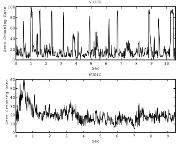
Saunders [5] used the Zero Crossing Rate, which is a good indicator of this behavior, as shown in Fig. 1.

The audio file is partitioned into segments of 2.04 seconds; each of them is composed of 150 consecutive non-overlapping frames. These values allow a statistical significance of the frame number and, using a 22050 Hz sample frequency, each frame contains 300 samples, which is an adequate trade-off between the quasi-stationary properties of the signal and a sufficient length to evaluate the ZCR.

For every frame, the value of the ZCR is calculated using the definition given in [5].

These 150 values of the ZCR are then used to estimate the following statistical measures:

• Variance: which indicates the dispersion with

respect to the mean value;

• Third order moment: which indicates the degree of

skewness with respect to the mean value;

• Difference between the number of ZCR samples, which are above and below the mean value.

Each segment of 2.04 seconds is thus associated with a 3-dimensional vector.

To achieve the separation between speech and music using a computationally efficient implementation, a multivariate Gaussian classifier has been used.

At the end of this step we obtain a set of consecutive segments labeled like speech or no-speech.

The next regularization step is justified by an empirical observation: the probability to observe a single segment of speech surrounded of music segments is very low, and viceversa. Therefore, a simple regularization procedure is applied to properly set the labels of these spurious segments.

The boundaries between segments of different classes are placed in fixed positions, inherently to the nature of the ZCR algorithm. Obviously these boundaries aren’t placed in a sharp manner, thus a fine-level analysis of the segments across the boundaries is needed to determinate a sharp placement of them. In particular, the ZCR values of the neighboring segments

are processed to identify the exact position of the transition between speech and music signal. A new signal is obtained from these ZCR values, applying this function

[ ]

[ ]

∑

Where x[n] is the n-th ZCR value of the current segment, and x_n is defined as:

[ ]

∑

Therefore y[n] is an estimation of the ZCR variance in a short window. A low-pass filter is then applied to this signal to obtain a smoother version of it, and finally a peak extractor is used to identify the transition between speech and music.

0 1 2 3 4 5 6 7 8 9 10 0 20 40 60 80 100 Sec

Zero Crossing Rate

VOICE 0 1 2 3 4 5 6 7 8 9 0 10 20 30 40 50 60 Sec

Zero Crossing Rate

MUSIC

Figure 1. The ZCR behavior for voice and music segments.

4.

NEURAL NETWORK CLASSIFIER

A Multi-Layer Perceptron (MLP) network [12] has been tailored to distinguish between music and speech. In multimedia applications mixed conditions must be managed, as music with a very rhythmic singer (i.e. rap song) or speech over music, as in advertising occurs. The MLP has been trained only by five kinds of audio traces, supposing other audio sources, as silence or noise, to be previously removed: pure music (class labeled as “Am”), melodic songs (class labeled as “Bm”), rhythmic songs (class labeled as “Cm”), pure speech (class labeled as “Av”) and speech superimposed on music (class labeled as “Bv”).

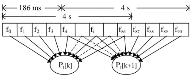
Eight features have been selected as the neural network inputs. These parameters have been computed considering 86 frames by 1024 points each (sampling frequency fs=22050Hz), with a total observing time of

frame buffer has been provided and features pj, in terms

of mean value and standard deviation, are updated every 186 ms, corresponding to 4 frames fi, as depicted in Fig.

2.

Figure 2. Features Pj updating frequency.

A short description of the eight selected features follows. Parameter P1 is the spectral flux, as suggested

by [13]. It indicates how rapidly changes the frequency spectrum, with particularly attention to the low frequencies (up to 2.5kHz) and it generally assumes higher values for speech.

Parameters P2 and P3 are related to the short-time

energy [14]. Function E(n), with n=1 to 86, is computed as the sum of the square value of the previous 1024 signal samples. A fourth-order high-pass Chebyshev filter is applied with about 100Hz as the cutting frequency. Parameter P2 is computed as the standard

deviation of the absolute value of the resulting signal, and it is generally higher in speech. Parameter P3 is the

minimum of the short-time energy and it is generally lower in speech, due to the pauses that occur among words or syllables.

Parameters P4 and P5 are related to the cepstrum

coefficients, as indicated in equation 1.

(1)

Cepstrum coefficients cj(n), suggested in [15] as

good speech detectors, have been computed for each frame, then the mean value c_µ(n) and the standard deviation cσ(n) have been calculated and parameters P4

and P5 result as indicated in equation 2.

P4=cµ(9)⋅cµ(11)⋅cµ(13), P5=cσ(2)⋅cσ(5)⋅cσ(9)⋅cσ(12) (2)

Parameter P6 is related to the spectral barycentre, as

music is generally more sensible in the low frequencies. In particular, the first-order-generalized momentum (barycentre) is computed starting from the spectrum module of each frame. Parameter P6 is the product of

the mean value by the standard deviation computed by the 86 values of barycentre. In fact, due to the speech discontinuity, standard deviation makes this parameter more distinctive.

Parameter P7 is related to the ratio of the

high-frequency power spectrum (7.5kHz<f<11kHz) to the whole power spectrum. The speech spectrum is usually considered up to 4kHz, but the lowest limit has been increased to consider signals with speech over music. To consider the speech discontinuity and increase the discrimination between speech and music, P7 is the ratio

of the mean value to the standard deviation obtained by the 86 values of the relative high-frequency power spectrum. Parameter P8 is the syllabic frequency

computed starting from the short-time energy calculated on 256 samples (≈12ms) instead of 1024. A 5-taps median filter has filtered this signal and P8 is the

number of peaks detected in 4s. As it is known [18], music should present a greater number of peaks.

To train and preliminarily test features and the MLP, a set of about 400 4s-long audio samples have been considered belonging to the five classes labeled as Am, Bm, Cm, Av, Bv and equally distributed between speech (Av, Bv) and music (Am, Bm, Cm). The discrimination power of the selected features has been firstly evaluated by computing index α, defined by equation (3), for each feature Pj, with j=1 to 8, where µm

and σm are respectively the mean value and standard

deviation of parameter Pj for music samples, and µv and

σv are the same for speech. α-values between 0.7 and 1

result for the selected features.

(3)

The selected MLP has eight input, corresponding to the normalized features P1÷P8, fifteen hidden neurons,

five output neuron, corresponding to the five considered classes, and uses normalized sigmoid activation function. The 400 4s-long audio samples have been divided in three sets: training, validation and test. Each sample is formatted as {P1÷P8, PAv, PBv, PAm, PBm, PCm},

where PAv is the probability that sample belongs to class

Av. The goal is to distinguish between speech and music and not to identify the class; for this reason target has been assigned with “1” to the selected class, “0” to the farest class, a value between 0.8 and 0.9 to the similar classes and a value between 0.1 and 0.2 to the other classes. For instance if a sample of Bm is considered, that is melodic songs, PBm=1, PAm= PCm=

0.8 because music is dominant, PBv = 0.2 because it is

anyway a mix of music and voice, and PAv= 0.1,

because the selected sample contains voice. If a pure music sample is considered (class Am), PAm=1, PBm= Cm= 0.8 because music is dominant, PBv = 0.1 because it

is anyway a mix of music and voice, and PAv= 0,

because pure speech is the farest class. In fact, classifying the speech over music as speech inclines the dw e e X n c

∫

MLP to classify as speech some rhythmic songs: by adjusting the sample target it is possible to incline to one side or another the MLP response. In this application we suppose to discriminate between speech and music to successively identify particular words from speech, so a light preference to speech is acceptable. The MLP has been trained by Matlab tools using the Levenberg-Marquardt method with a starting

µ value equal to 1000. The decision algorithm is depicted in Fig. 3. The mean error related to the 400 samples is 4%.

Figure 3. The decision algorithm.

5.

SIMULATION RESULTS

The proposed algorithms have been tested by computer simulations to measure the classification performance. The tests carried out can be divided in two categories: the first one is about the misclassification errors, while the second one is about the precision in music-speech and speech-music change detection.

Considering the misclassification errors, we defined three parameters as follow:

• MER (Music Error Rate): it represents the ratio between the total duration of the segments misclassified, and the total duration of the test file.

• SER (Speech Error Rate): it represents the ratio between the total duration of the segments misclassified, and the total duration of the test file.

• TER (Total Error Rate): it represents the ratio between the total duration of the segments misclassified in the wrong category (both music and speech), and the total duration of the test file. The “generation” of the test files was carried manually, i.e., each file is composed of many pieces of different types of audio (different speakers over different enviromental noise, different kinds of music as classical, pop, rap, funky,…) concatenated in order to have five minutes segment of speech followed by five minutes segment of music, and so on, for a total duration of 30 minutes.

All the content of this file has been recorded from a FM radio station, and it has been sampled at a frequency of 22050 Hz, with a 16 bit uniform quantization.

The classification results for both the proposed methods

are shown in Table 1.

MER SER TER

MLP 11.62% 0.17% 6.0%

ZB 29,3% 6,23% 17.7%

Table 1. Classification results of the proposed algorithms (MLP: Multi Layer Perceptron; ZB: ZCR with Bayesian Classifier).

From the analysis of the simulation results, we can see that, the MLP method gives better results compared to the ZB one, having a lower error rate both in music and speech.

Moreover, both the methods show the worst performance in the classification of the music segments, i.e., many segments of music are classified as speech than viceversa.

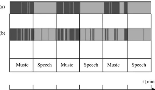
For a better understanding of these results, it can be useful take a look to the Fig. 4.

Figure 4. Graphical display of the classification results (a: MLP, b: ZB).

In the first row are shown the classification results of the MLP algorithm, where the white intervals are the segments classified as speech and the black ones are the segments classified as music.

The second row shows the classification results obtained using the ZB algorithm.

From the figure, it appears clearly that the worst classifications are carried out in the third music segment, between the minutes 20 and 25. The explanation is that these pieces of music are styles containing strong voiced components, under a weak music component (rap and funky).

The neural network makes a mistake only with the rap song, while the ZB approach performs a misclassification with the funky song too.

This is due mainly to these reasons:

• The MLP has been trained to recognize also music M L P MAX MAX P P P P P P P P PAm PBm PCm PAv PBv Pm Pv y≥0, music y<0, speech y

Music Speech Music Speech Music Speech

t [min] (a)

with a voiced component, and it gets wrong only if the voiced component is too rhythmic (e.g., rap song in our case). On the other hand, the Bayesian classifier used in the ZB approach does not take in account cases with mixed component (music and voice), and therefore in this case the classification results are significantly affected by the relative strongness of the spurious components.

• Furthermore, the ZB approach, that uses very few parameters, is inerently not able to discriminate between pure speech and speech with music background, while the MLP network, which uses more features, is able to make it.

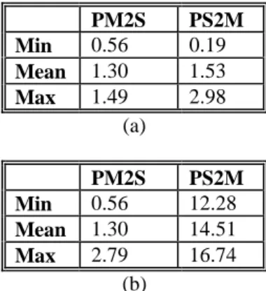
Considering the precision of music-speech and speech-music change detection, we measured the distance between the correct point in the time scale when a change occurred, and the nearest change point automatically extracted from the proposed algorithms. In our specific test set, we have only five changes, and we have measured the maximum, minimum and the mean interval between the real change and the extracted one. The results are shown in Table 2, where PS2M (Precision Speech to Music) is the error in speech to music change detection, and PM2S (Precision Music to Speech) is the error in music to speech change detection. PM2S PS2M Min 0.56 0.19 Mean 1.30 1.53 Max 1.49 2.98 (a) PM2S PS2M Min 0.56 12.28 Mean 1.30 14.51 Max 2.79 16.74 (b)

Table 2. MLP (a), and ZB (b) change detection results expressed in seconds.

Also in this case, the MLP obtain better performance than the ZB.

6.

CONCLUSION

In this paper we have proposed and compared two different algorithms for audio classification into speech and music. The first method is based mainly on ZCR and Bayesian Classification (ZB), and is very simple from the computational point of view.

The second approach uses Multi Layer Perceptron (MLP), and considers more features, requiring therefore more computations. The two algorithms have been tested to measure its classification performance in terms of misclassification errors and precision in music-speech change detection. Both the proposed algorithms give good results, even if the MLP shows the best performance.

REFERENCES

[1] MPEG Requirement Group. MPEG-7: Overview of the MPEG-7 Standard. ISO/IEC JTC1/SC29/WG11 N3752, FRANCE, Oct. 1998.

[2] C. Saraceno, R. Leonardi, “Indexing audio-visual databases through a joint audio and video processing”, International Journal of Imaging Systems and Technology, no. 9, vol. 5, pp. 320-331, Oct. 1998.

[3] N. Adami, A. Bugatti, R. Leonardi, P. Migliorati, L. Rossi, “Describing Multimedia Documents in Natural and Semantic-Driven Ordered Hierarchies”, Proc. ICASSP'2000, pp. 2023-2026, Istanbul, Turkey, 5-9 June 2000.

[4] A. Bugatti, R. Leonardi, L. A. Rossi, “A video indexing approach based on audio classification”, Proc. VLBV´99, pp. 75-78, Kyoto, Japan, 29-30 Oct. 1999. [5] J. Saunders, “Real Time discrimination of broadcast music/speech”, In Proc. ICASSP’96, pp. 993-996, 1996.

[6] E. Scheirer, M. Slaney, “Construction and

evaluation of a robust multifeature speech/music discriminator”, In Proc. ICASSP’97, 1997.

[7] J. Foote, “A similarity measure for automatic audio classification”, In Proc. AAAI'97 Spring Symposium on Intelligent Integration and Use of Text, Image, Video and Audio Corpora, 1997.

[8] C. Saraceno. Content-based representation and

analysis of video sequences by joint audio and visual characterization. PhD thesis, Brescia, 1998.

[9] T. Zhang, C. C. Jay Kuo, “Content-based

classification and retrieval of audio”, SPIE Conference on Advanced Signal Processing Algorithms, Architectures and Implementations, 1998.

[10] Z. Liu, J. Huang, Y. Wang, T. Chen, “Audio features extraction and analysis for scene classification”, Workshop on Multimedia Signal Processing, 1997.

[11] J.L. Gauvain, L. Lamel, G. Adda, “Partitioning and Transcription of Broadcast Data”, ICSLP, pp. 1335-1338, 1998.

[12] S. Haykin, “Neural Networks, a comprehensive foundation”, Prentice Hall, 1999.

[13] E. Scheirer, M. Slaney, “Construction and

evaluation of a robust multifeature speech/music discriminator”, Proc. of the 1997 ICASSP, Munich, Germany, April 21-24, 1997.

[14] L.R. Rabiner, R.W. Shafer, “Digital processing of speech signals”, Prentice Hall.

[15] L.R. Rabiner, “Fundamental of speech recognition”, Prentice Hall, 1999.