Un grande abbraccio a tutta la mia famiglia che mi ha seguito durante questi cinque anni di studio. Grazie di tutto.
Contents
1 Introduction 5
1.1 Current surveillance technologies . . . 5
1.2 WiCa smart camera . . . 8
1.2.1 IC3D . . . 8
1.3 8051 microcontroller . . . 10
1.4 DPRAM . . . 10
2 Architecture 13 2.1 Network Architecture . . . 13
2.2 The WiCa platform . . . 14
2.2.1 Win32 application . . . 15
2.3 Communication language . . . 18
2.3.1 The WiCa packet . . . 18
3 WiCa 19 3.1 The IC3D . . . 19
3.1.1 Extrapolation and interpolation . . . 20
3.1.2 Stereo background subtraction and silhouette . . . 22
3.1.3 Stereo vision . . . 24 3.1.4 Calibration . . . 26 3.1.5 Face detection . . . 27 3.2 Microcontroller 8051 . . . 30 3.2.1 8051 interconnections . . . 30 3.2.2 8051 kernel . . . 31
4 The distributed surveillance algorithm 33 4.1 Introduction . . . 34
4.1.1 Smart Cameras network . . . 34
4.2 Algorithm . . . 35
4.3 Mathematical proof . . . 40
4 CONTENTS
A Implement a command on the WiCa platform 45
A.1 Win32application.c . . . 46
A.2 8051application.c . . . 47
A.3 IC3Dapplication.xtc . . . 48
B Implementation of the algorithms in the IC3D 51 B.1 Extrapolation and interpolation . . . 51
B.2 Stereo background subtraction and silhouette . . . 52
B.3 Stereo Vision . . . 54 B.4 Calibration . . . 54 B.5 Face detection . . . 54 C Zigbee 57 C.1 Devices type . . . 57 Bibliography 59
Elenco delle figure 63
Chapter 1
Introduction
Electronic surveillance has become an important part of the workplace. Offices, banks, factories, retail outlets, and restaurants commonly use some form of elec-tronic surveillance to watch their workplace and employees. These methods of surveillance range from cameras and videotaping, electronic tracking devices in motor vehicles and cell phones, telephone and computer monitoring to biomet-ric identification. Next chapter shows the current surveillance technologies, in particular having a look to the benefits and limitations.
1.1
Current surveillance technologies
There are three types of surveillance technology to consider:
Analog/Time Lapse Systems : As depicted in Figure 1.1 on the following page Monitors are analog TV monitors which can display one video signal. In other words they have one video input. They are nothing more than high resolution TV’s. They range in size from 9" to 25" screens. They are the only way to view cameras with a time lapse recording system. With the addition of a multiplexer you can display 4, 9 or 16 video signals on one monitor. The multiplexer only provides the ability to view multiple cameras on one screen. It does not provide the ability to record.
With the addition of a Time Lapse Recorder, Figure 1.2 on the next page, it is possible record the video signal from a single camera, or a multi-camera view from a multiplexer using a standard VCR tape. Time Lapse Recorders
6 Introduction
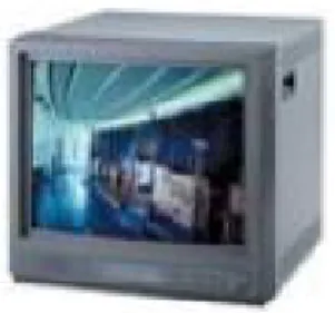
Figure 1.1: Color analog monitors.
are available in several different versions. Some even record up to 960 hours on 1 VCR tape, but it can be recorded on it only 1 frame or picture every 9 seconds.
Figure 1.2: Time Lapse Recorder.
The systems are very reliable and no computer skills are required to operate them, but the video quality is considered fairly low compared to the digital systems, the tape must be changed every three days or more, the system requires regular cleaning and maintenance on the VCR, the video quality degrades over time and the systems do not have the ability for networking or remote viewing.
PC Based Digital Video Systems : A PC based DVR is comprised of a com-puter, video capture cards and custom written software. These systems are considered to be the best bang for the buck. They provide far better video recording clarity over Time Lapse and are easier to use and more flexible than Hardware DVR’s. These units are available as kits which you install on your PC or as complete factory built recorders. Some factory models can be expanded as your needs grow, this is not the case with Time Lapse or Hardware DVR’s.
PC based DVR’s are programmed and operated with a keyboard and mouse. The video is recorded to the computers hard drive in a compressed format.
1.1 Current surveillance technologies 7
This compression allows a huge amount of video to be stored. On average, a four camera system recording continuously should record at least 30 days of video for all 4 cameras on one single 80 gig hard drive. To double the recording days simply add another 80 gig hard drive. These systems are designed so they do not require any scheduled action to maintain the video recordings. They record video to the hard drive until a certain amount of disk space is left. Then the system will delete the oldest clips and record the new video. This provides a continuous 30+ days of recordings at anytime.
Hardware Based Digital Video Systems : A hardware based DVR is built specifically for video recording. These units are built from the ground up to perform one specific function, record video. While they do operate some software internally, the video processing is hardware based. It is this hardware which provides the live viewing and high resolution recording. Hardware DVR’s are available in two different versions. The older style looks much like a VCR but has a hard drive built into it to record the video. A TV or CCTV analog monitor is used to view the video. Their programming is much like a VCR and can be quite confusing. The basic rule with this type of unit is, the more features they have the harder they are to operate. Most are programmed with a hand held remote much like a regular VCR. They do provide high resolution digital recordings which match the quality of a PC based DVR.
In this report it will be show the next generation architecture in surveillance system using smart camera. This devices are able to accomplish varying opera-tions while they are capturing the images. Indeed the system it is able to gather up the relevant informations of what it is aquiring. Because the camera can un-derstand what they are looking at, it is not necessary record all the video, but only what the user wants.
The next section introduce the WiCa smart camera, looking at the main features and capability that makes this device suitable to be used in a surveillance system.
8 Introduction
1.2
WiCa smart camera
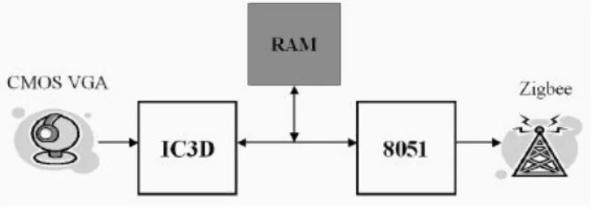
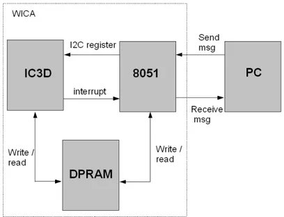
The WiCa smart camera is developed in the research laboratories of Philips Semi-conductor (now NXP). WiCa is a low power consumption and high performance smart camera for real-time video processing. The platform combines a SIMD processor (Philips IC3D) for low-level operations, an 8051 microcontroller for intermediate and high level operations and a Zigbee transmitter for communica-tion.
The low-level is associated with typical kernel operations like convolutions and data dependent operations using a limited neighbourhood of the current pixels. Due to the high degree of parallelism, a SIMD processor is best suited to accomplish this type of tasks. In the high- and intermediate-level part of image processing, decisions are made and forwarded to the user. General purpose processors are ideal for these tasks because they offer the flexibility to implement complex software tasks and they are often capable of running an operating system and doing networking applications.
This platform is capable of handling video streams at 25 frames per second with a power consumption of less than 200mW. A schematic of the architecture is depicted in Figure 1.3.
The WiCa has a Zigbee transceiver to handle the communication tasks.
Figure 1.3: The WiCa architecture. Between the processors there is a shared DPRAM memory.
1.2.1
IC3D
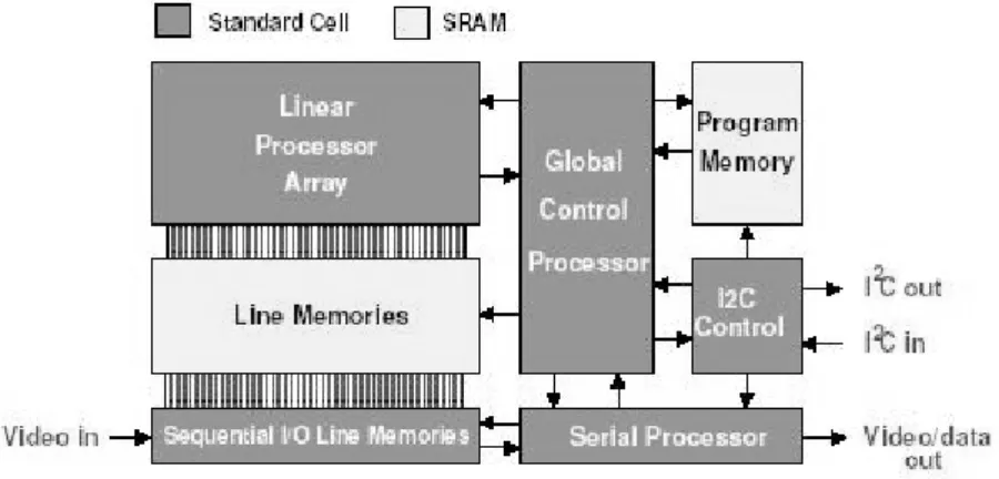
The Xetal IC3D IC is specificly designed to perform pixel processing on line based video data. The chip consists of a global control processor (GCP), a digital input
1.2 WiCa smart camera 9
processor (DIP), a digital output processor (DOP) and a linear processor array (LPA). This LPA has 320 pixel processors (PP) working in parallel. Besides these processors the IC3D has 64 linememories which can store a video line of 320 pixels and an instruction memory that can hold 2048 instructions. Internally the IC3D is runnning at 80MHz and is able to achieve a performance of 50GOps. Programs for IC3D are written in a language named XTC which is basically C with some added structures for vector processing. Figure 1.4 shows the internal architecture.
Figure 1.4: IC3D architecture.
The DIP (Sequential I/O Line Memories) stores the video data coming from the image sensor. Then the GCP gives the command to transfer the line memory to the processing memories (Line memories block) where it will be processed. After the processing, the GCP copy the line memory in the DOP where it will be outputted. The copying actions from DIP/DOP to/from IO memories are a stand-alone internal operation, where GCP only activates this process. The copying between IO and processing memories is done under total control of the GCP program.
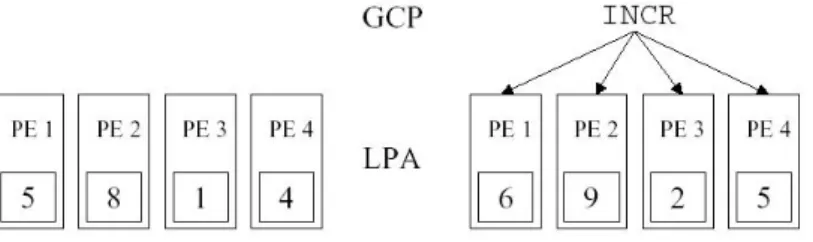
Single Instruction Multiple Data
IC3D is a parallel chip working in SIMD mode. Single Instruction Multiple Data (SIMD) is a technique that makes use of the inherent data parallel execution patterns in pixel-type processing. A SIMD processor contains many processing elements (PEs) combined into a Linear Processor Array (LPA). Each PE performs
10 Introduction
the same operation only on different data.
Figure 1.5: SIMD example.
An example can be seen in Figure 1.5. In this example there is a processor array with four processors and some arbitrary values from a linememory where the processors operate on. They receive the instruction increment and all processors execute it in parallel. If the same operation should be done on a general purpose processor it would require four times as many cycles, if we neglect overhead from instruction and operand-fetches.
1.3
8051 microcontroller
The 8051 is the control processor for the WiCa . This microcontroller is an AT89C51ED2 processor from Atmel running at 24MHz and is used for commu-nicating to the Aquis Grain Zigbee device, programming the IC3D and carrying out high level image operations.
1.4
DPRAM
The DPRAM on theWiCa is a 128K x 9 Dual Port Static RAM (IDT70V19). Since both the 8051 and the IC3D have 16 address lines they can address only up to 64KB of this external memory. Two output pins from the 8051 are connected to the two MSB address bits on both sides of the DPRAM to effectively divide the DPRAM in two 64KB banks. This makes it possible for the 8051 to control which bank the IC3D is reading/writing to, so the 8051 and IC3D can work in parallel on different banks of the memory. At each address 9 bits can be stored, but since pixelvalues only range from 0-255 only the 8 lowest bits are used.
1.4 DPRAM 11
The DPRAM can be accessed via the IC3D and the 8051. The IC3D has 24 data output lines. The 8 lowest lines are connected to the datalines of the DPRAM and the other 16 lines are used for addressing. Reading from and writing to DPRAM can be disabled for the IC3D by setting P4_5 to VDD. In this way the 8051 can block memory access for the IC3D when a new program for the IC3D is being written to memory. During programming 8KB of memory is reserved for the IC3D-program starting at address 0x0000 and 2 bytes are reserved for writing the size of the program at address 0x2000. Once a program has been sent to the IC3D, this part of the memory (0x0000 - 0x2001) can be used. This might lead to a programming hazard when one wants to switch IC3D programs dynamically and load a new program from the EEPROM. The memory contents on the addresses 0x0000 to 0x2001 will be overwritten.
Chapter 2
Architecture
This chapter describes the network architecture where it runs the self-localizing camera network algorithm. Also, it has been developped a WiCa platform to build distributed applications on this type of network. The end of the section describes the communication language used
2.1
Network Architecture
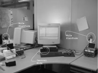
Figure 2.1 on the next page shows an example of smart camera network set up. As we can see from the figure, there are two main types of devices. The smart camera used for the video processing and the central node used to process the data coming from the smart camera. With the Zigbee protocol two smart camera can’t communicate each other. The central node serve as central unit to accomplish the video distribution tasks.
While the network is running, three main parts communicate each other. The Win32 application that implements all the functionality of the central node, the microcontroller that works like a bridge between the IC3D and the application and it realize some high level task, and the IC3D for the low level operation (video processing).
Even if in this application we use only two cameras, the architecture is com-plete independent from the number of smart camera used. This make the system very scalable and it makes the network easy for upgrades.
It has been built a framework to make easier the implementation and the debugging of the applications. This help us to debug the communication between
14 Architecture
Figure 2.1: The set up include two WiCa platforms and a central node(PC). Every node of the network is provide by a Zigbee transceiver.
the devices and the device itself. The next section describe this IDE.
2.2
The WiCa platform
The main purpose of this platform is to make easier the development of an appli-cation using WiCa smart cameras and expecially for distributed video processing. This platform helps during the programming phase thanks also to a simple debug environment. The high level viewing of the architecture see three main parts that communicate each other. The Win32 application, the 8051 microcontroller and the IC3D processor. These together form the complete architecture as we can see from Figure 2.2 on the facing page
The PC(Win32 application) and the microcontroller can communicate sending messages. The messages are built upon packets (this is explained in the next section). In particular, the microcontroller can send messages only to reply to messages sent by the PC. So the central unit works like a referee for the network, it gives commands to the WiCa for run some particular application and it controls the communication in the network giving the right timing.
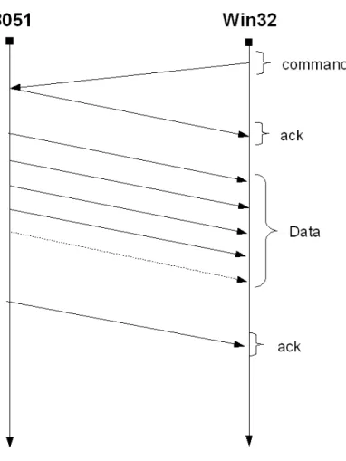
To guarantee the accuracy of the communication, The Win32 application and the 8051 follow a simple communication protocol as described in Figure 2.3 on page 16.
2.2 The WiCa platform 15
Figure 2.2: Architecture framework
the microcontroller reply with an ack to advise the PC that the microcontroller received the command. After, the microcontroller start to transfer data if it needs, otherwise it send another ack to advise the PC that the microcontroller finish to process the command and terminate the communication.
In the case of a broadcast signal no ack is sent by any Wica. This prevent the formation of a noisy signal made by the superimposition of the ack signal sent by all the Wica in the network.
The next part explain the framework in each kernel and it gives a global viewing to build applications on the platform.
2.2.1
Win32 application
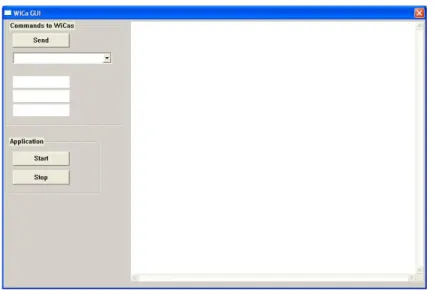
Figure 2.4 on page 17 shows the Win32 application interface to the WiCa devices. The figure shows the WiCa GUI application. The application is separate in three main parts:
debug box : it’s the big white box on the right. It shows what happen in the network, which camera sent a particulare message and if the applica-tion receive acknowledgement. It can be also customized to shows other information during a command process.
16 Architecture
Figure 2.3: Communication protocol between the Win32 application and the 8051 microcontroller.
2.2 The WiCa platform 17
Figure 2.4: Win32 application. It is the communication interface to the WiCa devices and it gives the opportunity to run a custom application.
Commands to Wicas : The first task executed by the application is to retrieve automatically the list of the command supported by the WiCas of the net-work. This list of commands appear in the combo box. Each entry of the menu has a number (the id of the WiCa, to identify which smart camera support that particular command) followed by a short string describing the functionality of the command, as depicted in figure 2.5
Figure 2.5: Combo box for the commands. The picture shows the commands supported by the two WiCa of id 70 and 202.
As we can see from the Figure 2.5 the user can select which command launch to a particular WiCa. In this case, for example, we can launch a command to retrieve the data from the DPRAM of the WiCa 202 or execute the calibration program from the WiCa 70.
If the microcontroller during the execution of the command wants to in-teract with the Win32 application, the user has the opportunity to write a
18 Architecture
function to carry out this task. To implement a command see the appendix A.
Application : The last part give the opportunity to launch an indipendent application built by the user. To have a good application running, it is better build the application as a list of command. This keep the program modular and it is more easy to debug. If a user has some problem with a command, he can run it as separate command from the WiCa commands section and see from the debug window what happens.
2.3
Communication language
The WiCa communication language is built upon the 802.15.4 MAC layer, and it is based on messages where each message is represented as packet.
2.3.1
The WiCa packet
The WiCa packet is included in a 802.15.4 MAC layer frame. The maximum payload of an 802.15.4 frame is 118 (see Figure 2.6). The Wica Header consists of 4 bytes as depicted in Figure 2.7, which leaves 114 for data. The 114 bytes data can also be used to extend the WiCa.
Figure 2.6: WiCa packet.
Chapter 3
WiCa
This section describe what it runs inside the WiCa, in particular we’ll speak about the IC3D kernel and the 8051 kernel. Then, it shall be shown the communica-tion protocol between these two processors and what informacommunica-tions is exchanged between them.
3.1
The IC3D
As it said before, the IC3D run the low-level operations. The processor receives one line memory at time (640 pixels for each RGB channel) from the image sensor. From a computer programming view an IC3D program appears as shown below 3.1.
Listing 3.1: A typical IC3D source code
1 // V a r a b l e s d e c l a r a t i o n 2 3 // I n i t i a l i z a t i o n 4 5 //Frame s y n c h r o n i z a t i o n 6 7 while ( 1 ) 8 { 9 //Frame i n i t i a l i z a t i o n 10 11 f o r e a c h row o f t h e f r a m e 12 { 13 // row s y n c h r o n i z a t i o n and r e a d i n g 14 // row c o m p u t a t i o n 15 } 16 }
20 WiCa
In the context of the surveillance system project the IC3D performs a series of tasks on the image acquired:
(a) Extrapolation and interpolation. (b) Stereo background subtraction. (c) Face detection.
(d) Silhouette. (e) Stereo vision.
Each operation will be treated in the next paragraphes.
3.1.1
Extrapolation and interpolation
To run a background subtraction algorithm we have to store the background in the memory. To accomplish this task the IC3D use the DPRAM memory, as depicted in Figure 1.3 on page 8. The DPRAM on the WiCa is a 128K x 9 Dual Port Static RAM (IDT70V19). Since both the 8051 and the IC3D have 16 address lines they can address only up to 64KB of this external memory. Two output pins from the 8051 are connected to the two MSB address bits on both sides of the DPRAM to effectively divide the DPRAM in two 64KB banks. So it is possible use one bank during a frame operation of 64KB.
The resolution of the screen is 640x480 pixels so it is not possible store a complete frame in one bank to implement a background subtraction algorithm (required 307200 Bytes). So, we use an extrapolation algorithm to compress the data to store in the memory and then, we apply an interpolation algorithm trying to rebuild the original line memory to use for the background subtraction.
Interpolation : In the most general meaning, interpolation is a method of constructing new data points from a discrete set of known data points. In image processing this comes usually down to reconstructing an unknown pixel value using information from its neighbors. On the IC3D we only save the pixels of the even video lines, on even pixelcolumns from pixelcolumns 64 to 574. Figure 3.1 on the facing page illustrates which pixels from the
3.1 The IC3D 21
Figure 3.1: This picture shows the interpolation process. (a) shows four interested pixels. (b) shows the vertical interpolation. (c) shows the horizontal interpolation
sensor are written to the memory (gray pixels are the pixels for which the data is saved).
By handling the pixel information in this way we are effectively decreasing the sample rate which might lead to aliasing errors. To avoid these aliasing errors normally a low pass filter is applied to the image before subsampling it. The lens also acts as a low pass filter which is at this time enough to suppress aliasing.
Extrapolation : It is the dual operation respect the interpolation. We choose only one row every two rows, and for each row we store in the memory only one pixel every two pixels as depicted in Figure 3.2
Figure 3.2: This picture shows the extrapolation process. The gray pixels are stored in the memory
22 WiCa
3.1.2
Stereo background subtraction and silhouette
A background subtraction algorithm reduce the probability of false positive detec-tion when the face detecdetec-tion is running and it improves the surveillance system separating the foreground (important informations) from the background. To accomplish this task we apply three operations:
background subtraction : An observed image is compared with an (estimate of the) image if it contained no objects of interest. The areas where there is a substantial difference between the observed image and the background are considered to be foreground. In the most basic application in a controlled environment first a picture is made of the background (B) and that one is subtracted for all the following images (It, t = 0, 1, . . .) where t denotes the
time index of the image. The subtraction of B and It generates a difference
image. The next step is applying a threshold (τ ) on the difference image to separate the background and foreground pixels (|It− B| > τ ).
erosion : Beacuse we work with a greyscale picture, we have a gradation of the colour of only 256 values and to separate well the background from the foreground we need a big value of the threshold τ . But, big value of the threshold increse the number and the size of black blobs in the image. To avoid this problem we apply before the background subtraction algorithm with a low value of the threshold and then we apply the erosion operation to the image. We don’t care about an eroded image, it is important instead delete the black blobs inside the foreground image.
Erosion is one of the two basic operators in the area of mathematical mor-phology, the other being dilation. It is typically applied to binary images, but there are versions that work on greyscale images. The basic effect of the operator in our context is to erode away the boundaries of regions of foreground pixels (i.e. white pixels, typically). Thus areas of foreground pixels shrink in size, and holes within those areas become larger but this blobs disappear when we apply the silhouette algorithm. Figure 3.3 on the facing page shows an example of erosion operation.
silhouette : The WiCa is provided by two image sensor. In the first solution only one background seen by the first image sensor has been stored in the
3.1 The IC3D 23
Figure 3.3: Erosion operation using a 3x3 kernel.
DPRAM. But the range between the two image sensors is too big and the sensor 2 see the same background but a little bit traslated, so the comparison between what the sensor 2 see and the background produce an imperfect background subtraction.
To remove completely the noise coming from the different viewing of the cameras, a stereo background subtraction is implemented. In this way, each image sensor store its background in the DPRAM. In this context the image sensor 1 and the image sensor 2 store the background in the DPRAM bank0 and DPRAM bank1 respectively.
Even if there are no more noise coming from the different viewing of the two image sensors, the background subtraction is not perfect yet. Infact, due to the threshold, black blobs can appear in some foreground zone with the conseguence that sometimes can disappear some piece of the body. To avoid this problem it was implemented a silhouette algorithm. The silhouette algorithm computes a mask that surrounds the foreground. After, in the next frame, this mask is applied in the manner that everything inside the countour of the mask becomes the foreground. If we apply the silhouette, everything below the mask is preserved getting a better foreground, as shown in Figure 3.4 on the next page.
However that may be lost areas where the blobs appear in the countour zone, because in that case the blob modify the mask as we can see from the right shoulder depicted in Figure 3.4 on the following page. To see the IC3D implementation of this algorithm, refer to appendix B.2.
24 WiCa
Figure 3.4: The Figure shows the background subtraction algorithm with the addition of the silhouette algorithm. Figure (a) shows background + foreground. Figure (b) shows the background. Figure (c) shows the background subtraction with the silhouette algorithm
3.1.3
Stereo vision
Stereo vision refers to the ability to infer information on the 3-D structure and distance of a scene from two or more images taken from different viewpoints.
Introduction
From a computational standpoint, a stereo system must solve two problems. The first, known as correspondence, consists in determining which item in the left eye corresponds to which item in the right eye. The second problem that a stereo system must solve is reconstruction. Our vivid 3-D perception of the world is due to the interpretation that the brain gives of the computed difference in retinal position, named disparity, between corresponding items. The disparities of all the image points form the so-called disparity map, which can be displayed as an image. If the geometry of the stereo system is known, the disparity map can be converted to a 3-D map of the viewed scene.
Stereo vision with parallel axes
Before starting our investigation of the corrspondence and reconstruction prob-lem, it is useful starts having a look to the stereo vision model depicted in Fig-ure 3.1.3 on the next page (a), this is the same set up of the WiCa smart camera. The diagram shows the top view of a stereo system composed of two pinhole cameras. The left and right image planes are coplanar, and represented by the segments Il and Ir respectively. Ol and Or are the center of the projections. The
3.1 The IC3D 25
Figure 3.5: Stereo vision with parallel axes. 3D reconstruction depends of the solution of the correspondance problem (a); depth is estimated form the disparity of corresponding points.
optical axes are parallel; for this reason, the fixation point, defined as the point of intesections of the optical axes, lies infinitely far from the cameras.
The way in which stereo determines the position in space of P and Q (Fig-ure 3.1.3) is triangulation, that is, by intersecting the rays defined by the centers of the projection and the images of P and Q, pr, pl, qr, ql. Triangulation depends
crucially on the solution of the correspondence problem: if (pl,pr) and (ql,qr) are
chosen as pairs of correspondence image points, intersecting the rays Olpl - Orpr
and Olql - Orqr leads to interpreting the image points as projections of P and Q;
but, if (pl,qr) and (ql,pr) are the selected pairs of corresponding points,
triangu-lations return P’ and Q’. Note that both interpretations, although dramatically different, stand on an equal footing once we accept the respective correspon-dences. Because only one point is in the FOV of the cameras when the algorithm is running, this problem is bypassed.
Because during the self-localizing camera network algorithm we have only one face that pass through the FOV of the WiCa cameras, the correspondance prob-lem is solved, so we have a look to the reconstruction probprob-lem. we concentrate
26 WiCa
on the recovery of a single point, P, from its projections, pl and pr (Figure 3.1.3
on the previous page (b)). The distance, T, between the centers of projections Ol and Or, is called the baseline of the stereo system. Let xl and xr be the
coor-dinates of pl and pr with respect to the pricipal points cl and cr, f the common
focal length, and Z the distance between P and the baseline. From the similar triangles (pl, P, pr) and (Ol, P, Or) we have
T + xl− xr Z − f = T Z (3.1) Solving 3.1 we obtain Z = fT d (3.2)
where d = xl − xr, the disparity, measures the difference in retinal position
between the corresponding points in the two images. From the Equation 3.2 we see that the depth is inversely proportional to disparity.
3.1.4
Calibration
As shown by Figure 3.1.3 on the preceding page, the depth depends on the focal length, f, and the stereo baseline, T; the coordinates xland xr are referred to the
principal points, cl and cr. The quantities f, T, cl, cr are the parameters of the
stereo system, and finding their values is the calibration problem.
Before calibrating the intrinsic parameters of the camera we have to shift the image coming from the sensor 2. Infact, due to a delay problem inside the WiCa architecture the frame captured by the image sensor 2 appears in the screen shifted by N pixels. The first thing so is to shift the image in the manner that image sensor 1 and image sensor 2 start to paint its frame from the same x coordinate position.
From the WiCa device we know that the stereo baseline T = 0.02 m. The disparity can be calculated using the face detection algorithm and saving the position of the x coordinate of the face for the image sensor 1 and image sensor 2. So we can compute the focal distance.
f = Zd
3.1 The IC3D 27
We choose to put the face in the middle of the two image sensors with a Z = 1m.
3.1.5
Face detection
A new feature based approach to detect faces in real-time applications using a massively-parallel processor architecture is introduced. The technique is based on a smooth-edges detection algorithm. The main advantage, when applied on intensity values, is that it is robust against homogonous variations of the illu-minating conditions. The algorithm run on both image sensors of the camera. This technique suffer of false positive detection error that are reduced apply-ing a background subtraction algorithm and some other filters explained in the next sections. The face detection is devided in two algorithm. A smooth edges detection algorithm to extract the main features from the image and a pattern recognition algorithm to find this features.
Smooth edge detection
Figure 3.6: (a) original image. (b) Position information provided by an edge detector.
In computer vision and image processing, edge detection concern the local-ization of significant variation of grey level image, as depicted in figure 3.1.5 and the identification of the physical phenomena that originated them. Usually, edge detection requires smoothing and differentiation of the image. Differentiation is an ill-conditioned problem and smoothing results in a loss of information. It is difficult to design a general edge detection algorithm which performs well in many
28 WiCa
contexts. Consequentely, we choose a edge detector that works well for retrieve the features of a face.
Conceptually, the most commonly proposed schemes for edge detection in-clude three operations:
Smoothing of the image : consists in reducing noise of the image and regu-larizing the numerical differentiation. Smoothing has a positive effect to reduce noise and to ensure robust edge detection; and a negative effect, information loss. We have a foundamental trade-off here between loss of information and noise reduction. In this section we will focus on linear filtering. The duration of the impulse response characterizes the support of the filter in the spatial or frequential domain. For instance, in edge de-tection, three kinds of linear low-pass filter have been used: band limited filters, support limited filters and filters with minimal uncertainty. The invariance to rotation property ensures that the effect of smoothing is the same regardless of edge orientation.
Image differentiation : Differentiation is the computation of the necessary derivatives to localize these edges to localize variation of the image grey level and to identify the physical phenomena which produced them. The differentiation operator is characterized by its order, its invariance to rota-tion and its linearity.
The most commonly used operators are the gradient, the Laplacian and the second-order directional derivative. For our purpose we choose the gradient operator defined as the vector (∂x∂ ,∂y∂).
Edge labeling : involves localizing edges and increasing the signal-to-noise ratio of the edge image by suppressing false edges. The localization procedures depends on the differentiation operator used. We choose to use the non-maximum suppression algorithm. The basic idea is to extract the local maxima of the gradient modulus. The algorithm used finds the local max-ima along the direction of the gradient vector. That is, if we consider the image plane as real, then a given pixel is a local maximum if the gradient modulus at this pixel is greater than the gradient modulus of two neigh-boring points situated at the same distance on either side of the given pixel along the gradient direction.
3.1 The IC3D 29
The elimination of false edges increases the signal-to-noise ratio of the differ-entiation and smoothing operations. While it may be true that the behavior of this operation depends on the performance of smoothing and differenti-ation and that these operdifferenti-ations are more and more robust, false edges do not originate only from noise. The rule commonly used to classify edges as true or false is that the plausibility value of true edges is above a given threshold. The threshold is the minimum acceptable plausibility value. Due to the fluctuation of the plausilbility measure, edges resulting from such a binary decision rule are broken. Two threshold are used; a given edge is true if the plausibility value of every edge point on the list is above a low threshold and at least one is above a high threshold.
Because the gradient differentiation operator is used, the plausibility mea-sure is the gradient modulus.
Figure 3.1.5 and 3.1.5 on the next page shows the above operations after apply the horizontal and vertical differentation operation respectively.
Figure 3.7: Image processed with a gaussian 3x3 smoothing filter and a horizontal diiferentiation operation.
Pattern recognition
At the end of the smooth edge detection process the image shows its edges. After a particular analysis we found that the face suggests a particular pattern that difficulty can be found in other zones of the image.
30 WiCa
Figure 3.8: Image processed with a gaussian 3x3 smoothing filter and a vertical differentiation operation.
3.2
Microcontroller 8051
AT89C51ED2 is high performance CMOS Flash version of the 80C51 CMOS single chip 8-bit microcontroller. It contains a 64-Kbyte Flash memory block for code and for data. The 64-Kbytes Flash memory can be programmed either in parallel mode or in serial mode with the ISP capability or with software. The programming voltage is internally generated from the standard VCC pin.
The microcontroller build into a TinyOS operating system. TinyOS is an open source component-based operating system and platform targeting wireless sensor networks. TinyOS is an embedded operating system written in the nesC programming language as a set of cooperating tasks and processes. It is designed to be able to incorporate rapid innovation as well as to operate within the severe memory constraints inherent in sensor networks.
3.2.1
8051 interconnections
Figure 3.2.1 on the facing page shows the principal interconnections of the mi-crocontroller with the devices. Using the i2c bus we can address the register of the image sensors that give us the opportunity to change some parameters of the aquiring sensor and the registers of the IC3D to pass some parameters to our
3.2 Microcontroller 8051 31
Figure 3.9: Microcontroller interconnections.
application. Also, the SPI send and receive data from the ZigBee transceiver for a Wireless communication and the IC3D can launch interrupt to the microcon-troller.
3.2.2
8051 kernel
The 8051 has a simple kernel started at boot. The major functionalities of the kernel are to handle communication, to configure the startup of the IC3D, to change parameters of the image sensors and to handle an application.
The kernel consists of a set of modulesdrivers which implements an interface to the underlying hardware. The basic functionality for the kernel is to watch the UART buffer (rxtx) to pass packets inout. Packets arriving from the AT128 are passed on to the packet manager for further handling and packets from the tx_queue are constantly scheduled for transmission. While the kernel is working, the application is disabled to provide consistent data in the memories. Following is described the several drivers.
Uart : This is an interrupt driven by the UART driver. It provides basic func-tionality to getput characters. Two internal buffers of the 128 bytes each handle the transmissionreceptions.
Queue : The queue is a module for incoming and outgoing packets. It is priority based where the priority flag in the packet header toggles priorities. The queues have internal packet pools, which are implementing so that the size is generic, but the current memory layout gives a size of 2∗4 packets.
32 WiCa
I2C : This module provides a hardware abstract layer. The module provides functionality to control the I2C bus.
EEPROM : This module provides functionality to readwrite both the internal and the external EEPROMs. There is also an interface to copy data between the external EEPROM and the DPRAM.
Memory : The memory module provides functionality to copy data between DPRAM and internal XRAM.
IC3D : This module provides all necessary functionality to control the IC3D, programming, instruction uploading, parameters settings, reset, onoff etc. Packet Manager : The packet manager provides functions to moves packets
between the two queues (rxtx) and the uart buffers (rxtx). This module is also responsible to parse incoming packets and distributed them to the applications ot to handle them internally in the kernel.
Chapter 4
The distributed surveillance
algorithm
This section describes formally the algorithm and how it is implemented using the WiCa. In this last part, we give particular attention to the communication protocol and we show which program run in the WiCa (IC3D and 8051 kernels) and PC.
To take full advantage of the images gathered from multiple vantage points it is helpful to know how the smart cameras in the scene are positioned and oriented with respect to each other.
The system uses WiCa smart cameras, a low power consumption and high-performance video processing devices, each one provided with two image sensors to implement a good algorithm for silhouette and face detection and a stereo vision algorithm to estimate the depth of the face detected.
In this paper it will be described that it is possible to know the relative position of all cameras in the network using only the depth information of a person who is walking through the FOV of the cameras. After having fixed the distance to the person of the cameras, the angle measurement is used to calculate their orientation.
This method makes easier the process of calibration using only video process-ing instead usprocess-ing any other device like infrared. So, this algorithm can help the installation of surveillance systems, for example.
34 The distributed surveillance algorithm
4.1
Introduction
This chapter describes how to locate the sensors in the network and what these sensors have to compute to make sure the algorithm runs properly. The only assumption is that each camera can estimate the angle and the depth of an object that is moving in the area of interest. Also, the syncronization between the cameras is important. Each one has to take the measurement at the same moment in time, depending on the motion of the object.
4.1.1
Smart Cameras network
Figure 4.1 show a small network of 4 nodes, three of which are smart cameras (C1, C2, C3) and one is the central node. This node is responsable for syncronizing the other nodes of the network, receiving the data and building the 2D map of the sensors. The viewing frustum of the cameras is limited by the fact that the face detection algorithm has a limited working range. Outside of this range it is neither possible to detect faces nor the depth and the angle.
Figure 4.1: Cameras network.
In Figure 4.1 two areas appear: A1 and A2. A1 is seen by all the cameras in the network, while A2 is seen only by the cameras C1 and C3. The black path is
4.2 Algorithm 35
an object moving in the area and the little spots (t0,t1,...,t5) are the instants of
time in which the position of the object is caught. We will refer to this picture during the description of the algorithm.
4.2
Algorithm
This section shows the algorithm with all the structure that it needs in order to work properly. The proof is given in the next section.
As said before, the central node builds the map describing the camera network. Without making any restriction it is presumed that all the cameras already made the measurement of the angle of view and depth of the face detected, for each instant of time t0, t1, ..., t5 and that all this information is already dispatched and stored in the central node. This data is displayed in table 4.1:
tj C1 C2 C3 t0 (dC1,t0,θC1,t0) 0 (dC3,t0,θC3,t0) t1 (dC1,t1,θC1,t1) 0 (dC3,t1,θC3,t1) t2 (dC1,t2,θC1,t2) (dC2,t2,θC2,t2) (dC3,t2,θC3,t2) t3 (dC1,t3,θC1,t3) (dC2,t3,θC2,t3) (dC3,t3,θC3,t3) t4 (dC1,t4,θC1,t4) (dC2,t4,θC2,t4) (dC3,t4,θC3,t4) t5 (dC1,t5,θC1,t5) (dC2,t5,θC2,t5) (dC3,t5,θC3,t5)
Table 4.1: Data received from smart cameras
Table 4.1 shows the data store in the central node. For each camera Ci and
instant of time tj the depth dCi,tj is stored and the angle θCi,tjof the object with
respect to the camera itself. If the camera is taking a picture and it doesnt’t detect any face in his FOV it specifies this case by storing the value 0.
To build a 2D map of the network it is necessary to know the relative position of the cameras. To find this information, the first thing is to specify a Cartesian plane with an origin point O of position (0,0). This point will be associated to the position of one camera. With this starting point and the data received from the cameras the central node will be able to attain the relative positions of the other cameras. The first camera chosen to start the computation is placed in the point (0,0) with the orientation versus the positive x-axis as depicted in Figure 4.2. All the positions of the other cameras will be found from that point and orientation.
36 The distributed surveillance algorithm
Figure 4.2: Cartesian plane and WiCa camera with position (0,0) and orientation versus positive x-axis
The central node builds a table to specify which cameras are already localized in the network as shown in the localization table 4.2
Ci localized position orientation
C1 no (xC1,yC1) ϕC1
C2 no (xC2,yC2) ϕC2
C3 no (xC3,yC3) ϕC3
Table 4.2: This example shows the localization table when the algorithm starts, so no camera has position and orientation in the Cartesian plane yet.
If the camera Ci is localized, the position (xCi,yCi) and the orientation ϕi in
the Cartesian plane is known and the associated field localization is put to the value yes otherwise the fields position and orientation have no meaning and the value is put to no.
After receiving the data and building the localization table the central node executes this iterative algorithm:
The algorithm starts looking for a camera not localized in the map. The camera must share at least three points (the mathematical prove is given in the next chapter) with another camera already localized that appear in the Table 4.3 on the next page. If no one is localized a camera is selected to put in the Cartesian plane as previously shown in Figure 4.2 on the facing
4.2 Algorithm 37
page and then go to step 2. If all the smart cameras are localized, the algorithm is terminated, otherwise a camera Ci is choosen that satisfies the
previous requirement and the algorithm returns to step 3. If no one of these conditions is met, another stream of object points is taken and everything restarts from the beginning.
The second step is to change coordinates from Local Space (camera space), where the points of the object are defined relative to the camera’s local origin (Figure 4.3), to World Space (Cartesian plane) where vertices are defined relative to an origin common to all the WiCas in the map (Figure 4.4 on the following page).
Figure 4.3: This example shows the Local Space of camera C1
Now the position of the chosen camera Ci is fixed, and it is possible to
fix the positions of the object seen by Ci in the Cartesian system. These
coordinates are saved in the World object space table as depicted in Table 4.3 on the next page.
These positions (xtj,ytj) are simply computed, in fact the depth between
the local space and the world space remains the same because the camera is in the origin of both spaces. Also the angle is similar for the local space because the orientation of the cam is equal to zero (ϕCi = 0) in the World
Space, so:
38 The distributed surveillance algorithm
Figure 4.4: This example shows the World Space after the positioning of C1 in the origin of the cartesian plane
tj world coordinates t0 (xt0,yt0) t1 (xt1,yt1) t2 (xt2,yt2) t3 (xt3,yt3) t4 (xt4,yt4) t5 (xt5,yt5)
4.2 Algorithm 39
ytj = dCi,tjsin (θCi,tj)
After this return to Step 1.
The camera Ci sees at least three world coordinates on the World Space.
As-suming that these points are related to these instants of time ti,tj,tk, from
the Table 4.3 on the facing page the following coordinates are taken: (xti,yti)
(xtj,ytj)
(xtk,ytk)
The following terms will simplify the resulting equations: a01= 2xtj − 2xti b01= 2ytj − 2yti c01= x2tj+ y 2 tj − d 2 Ci,tj− x 2 ti− y 2 ti + d 2 Ci,ti a02= 2xtk − 2xti b02= 2ytk − 2yti c02= x2tk+ y 2 tk − d 2 Ci,tk− x 2 ti− y 2 ti + d 2 Ci,ti
The position (xCi,yCi) of the camera Ci is computed by the following
Equa-tions: xCi = b02c01− b01c02 a01b02− b01a02 (4.1) yCi = a01c02− a02c01 a01b02− b01a02 (4.2)
40 The distributed surveillance algorithm formulas: x = (xti− xci) cos (−θCi,ti) − (yti − yCi) sin (−θCi,ti) (4.3) y = (yti− yCi) cos (−θCi,ti) + (xti− xCi) sin (−θCi,tj) (4.4) ϕCi = arctan ( y x) (4.5)
The arctan (yx) is implemented as Lookup Table(LuT). For x = 0, the arctan (xy) is equal to π/2 or −π/2 if y is rispectively positive or nega-tive. The next step is to fill the Localization table 4.2 on page 36 with the values obtained by the equations 4.1 on the preceding page, 4.2 on the previous page, 4.5 and to go back to Step 1.
4.3
Mathematical proof
This chapter proves how it is possible to calculate the position of one camera Ci
having knowledge of the position (X,Y) of three points (xti,yti), (xtj,ytj), (xtk,ytk)
and the distances dCi,ti, dCi,tj, dCi,tk from the camera to these points.
Figure 4.5 on the next page shows that having one point and the relative distance between this and the camera Ci is not enough to locate the camera
in space. In fact, the points that satisfy the distance dCi,ti are the points of a
circumference, described by Equation 4.6.
(x − xti)
2
+ (y − yti)
2
= d2Ci,ti (4.6)
Figure 4.6 on the next page shows a better situation using two points. In fact, now only two coordinates satisfy dCi,ti and dCj,tj in the same time. These
4.3 Mathematical proof 41
Figure 4.5: The figure shows that with one point, all points on the circle can be assigned as position of the camera.
Figure 4.6: This case shows that with two points the camera can be found only in the yellow spots.
42 The distributed surveillance algorithm (x − xti) 2+ (y − y ti) 2 = d2 Ci,ti (x − xtj) 2+ (y − y tj) 2 = d2 Ci,tj (4.7)
Figure 4.7: With three points the problem is solved and it exists only one solution shown by the yellow spot. This is the place where the camera is placed.
Figure 4.7 shows the case using three points. The solution exists and it is unique. The solution is given by:
(x − xti) 2+ (y − y ti) 2 = d2 Ci,ti (x − xtj) 2+ (y − y tj) 2 = d2 Ci,tj (x − xtk) 2+ (y − y tk) 2 = d2 Ci,tk (4.8)
This system could be computational expensive, but it can be simplified by the fact that the solution exists. Subtracting the first equation with the second equation of the System 4.8 a straight line A is obtained as depicted in Figure 4.7. Doing the subtraction between the second and the third equation of the same system the straight line B is obtained. Now, it needs only the following simple system of two linear equation needs to be solved.
4.4 Applications and future work 43 x(2xtj − 2xti) + y(2ytj − 2yti) + x 2 ti + y 2 ti −x2 tj − y 2 tj − d 2 Ci,ti + d 2 Ci,tj = 0 x(2xtk − 2xtj) + y(2ytk − 2ytj) + x 2 tj + y 2 tj −x2 tk − y 2 tk − d 2 Ci,tj+ d 2 Ci,tk = 0 (4.9)
The Equations 4.1 on page 39, 4.2 on page 39, 4.5 on page 40 are obtained from the System 4.9.
4.4
Applications and future work
Our set up is provided by two Wica cameras, as depicted in Figure 2.1 on page 14, each one provided with two image sensor and a central node(PC). Each node of the network communicates using a Zigbee transceiver.
In this stage a face detection algorithm is accomplished, as shown in Figure 4.8 and the low-level infrastructure to send packets of data between the devices. Also the communication protocol is working. We are working on mapping the part where the central node has to process the data to build the 2D map.
Figure 4.8: The figure shows the face detection algorithm running on WiCa platforms. The white stripe on the faces shows the detection of the faces.
Appendix A
Implement a command on the
WiCa platform
Chapter 2 gives an high level view of the WiCa platform, describing the tasks for each device (IC3D, 8051 and central unit) and it shows the communication protocol between them. This appendix is a step by step guide to implement a command on the WiCa platform. The user has to write the code of three files:
IC3Dapplication.xtc : this is the ic3d kernel file where it resides the IC3D application. There’s not a IDE to write the code for this file. The user is free to choose his favourite text processor. After writing the code, the user has to compile the program and then then he has to upload it using these commands from the shell:
1 > go I C 3 D a p p l i c a t i o n
2 > w ic a p − f bank WiCa_id I C 3 D a p p l i c a t i o n . b i n
Where IC3Dapplication is the IC3Dapplication.xtc file without the ex-tension. bank is one of the 8 free banks to save an IC3D application (the bank start from 0 to 7). The WiCa_id is an id of a WiCa and IC3Dapplication.bin is the binary file generated from the IC3D compiler. 8051application.c : This file is part of a µVision project.
Win32application.c : This file is part of a DEV C++ project. After compile the kernel, to program the 8051 execute the following command:
1 > go I C 3 D a p p l i c a t i o n
46 Implement a command on the WiCa platform
Where WiCa_id is the id of the WiCa device and kernel.hex is the intel hexfile generated by the Keil compiler.
The next sections describe what part of the code modify in these files.
A.1
Win32application.c
How it has been previously said, the Win32 application retreives automatically the commands from the WiCa. Anyway, some commands needs an handler to be processed or to follow a particular communication protocol. The code shows how to create a command handler.
1 .
2 .
3 .
4
5 // ID_COMMAND_CODE : T h i s c o s t a n t a d d r e s s a command managed by
6 // t h e 8 0 5 1 . The v a l u e id_command i s d e c l a r e d i n t h e 7 // 8051 a p p l i c a t i o n . c f i l e . 8 #d e f i n e ID_COMMAND_CODE id_command 9 10 . 11 . 12 . 13
14 // D e c l a r e t h e f u n c t i o n t h a t manage t h e command . The f u n c t i o n s
15 // can h a v e any name .
16 b o o l commandID_COMMAND_CODE( void ∗ p a r a m e t e r s ) ; 17 18 . 19 . 20 . 21
22 // Process_command i s t h e f u n c t i o n where t h e command i s managed . 23 //The c a l l i n g t o t h e f u n c t i o n command ( ) i s i n s i d e t h e c a s e
24 // c o n s t r u c t a s shown b e l o w .
25 b o o l process_command ( unsigned i n t i d , unsigned char command ,
26 void ∗ arguments , unsigned char p1 ,
27 unsigned char p2 , unsigned char p3 )
28 { 29 . 30 . 31 . 32 33 switch ( command ) 34 { 35 case ID_COMMAND_CODE: 36 commandID_COMMAND_CODE( a r g u m e n t s ) ;
A.2 8051application.c 47 37 break ; 38 } 39 40 . 41 . 42 . 43 44 return t r u e ; 45 }
A.2
8051application.c
This file specify the behavior of the microntroller to commands received by the Win32 application. In particular it can communicate with the PC sending data through messages or it can communicate with the IC3D processor using the I2C bus, the interrupt, or the shared DPRAM. The code explain all these aspects.
1 // T h i s e x a m p l e shows a l s o , a b r o a d c a s t command ( i t i s a 2 // command r e c e i v e d by a l l t h e WiCa i n t h e n e t w o r k ) 3#d e f i n e ID_COMMAND_CODE id_command 4#d e f i n e ID_COMMAND_CODE_BROADCAST id_command_broadcast 5 6 . 7 . 8 . 9 10 // a p p l _ i s r ( ) − A p p l i c a t i o n I n t e r r u p t S u b r o u t i n e 11 // 12 // T h i s i s t h e i s r c o n n e c t e d t o t h e e x t e r n a l i n t e r r u p t 13 // g e n e r a t e d by t h e i c 3 d . The i n t e r r u p t i s by d e f a u l t 14 // s e t on .
15 void a p p l _ i s r ( void ) i n t e r r u p t IC3D_INTERRUPT
16 { 17 // c o d e h e r e 18 } 19 20 . 21 . 22 . 23 24 // appl_main ( ) − Main a p p l i c a t i o n 25 // 26 // T h i s i s t h e main a p p l i c a t i o n . The a p p l i c a t i o n w a i t s f o r 27 // a p a c k e t . I f a p a c k e t a r r i v e , t h e a p p l i c a t i o n p r o c e s s i t 28 // o t h e r w i s e i t can do o t h e r c o m p u t a t i o n s .
29 void appl_main ( void ) _task_ TASK_APPL_MAIN
30 {
48 Implement a command on the WiCa platform 32 { 33 // w a i t i n g f o r a message 34 while ( ! pm_receive_wp(& a p p l _ i n _ b u f f e r ) ) 35 { 36 // i f no p a c k e t a r r i v e do o t h e r c o m p u t a t i o n s 37 } 38 39 // c h e c k w h i c h message h a s b e e n r e c e i v e d and t h e n s t a r t 40 // t h e c o m p u t a t i o n 41 i f ( a p p l _ i n _ b u f f e r . l e n g t h == 0 x04 && 42 a p p l _ i n _ b u f f e r . p a y l o a d [ 0 ] == ID_COMMAND_CODE) 43 { 44 // f i r s t Ack t o e n s u r e t h e r e c e p t i o n o f command 45 send_ack ( 0 x00 , TOKEN) ; 46 47 // p r o c e s s t h e command 48 49 // s e c o n d Ack t o c o m p l e t e t h e t r a n s f e r o f d a t a 50 send_ack ( 0 x00 , TOKEN) ; 51 } 52 i f ( a p p l _ i n _ b u f f e r . l e n g t h == 0 x04 && 53 a p p l _ i n _ b u f f e r . p a y l o a d [ 0 ] == ID_COMMAND_CODE_BROADCAST) 54 { 55 // p r o c e s s t h e command 56 }
57 //To add a command u s e t h e AddCommand f u n c t i o n
58 // i n t h i s s e c t i o n 59 e l s e i f ( a p p l _ i n _ b u f f e r . l e n g t h == 0 x04 && 60 a p p l _ i n _ b u f f e r . p a y l o a d [ 0 ] == 0xFF ) 61 { 62 // f i r s t Ack t o e n s u r e t h e r e c e p t i o n o f command 63 send_ack ( 0 x00 , 0xFF ) ; 64 65 //Add h e r e t h e commands 66 AddCommand(ID_COMMAND_CODE, " C o m m a n d ID " , 1 0 , 0 ) ; 67 AddCommand(ID_COMMAND_CODE_BROADCAST, 68 " C o m m a n d ID b r o a d c a s t " , 2 0 , 1 ) ; 69 70 // s e c o n d Ack t o c o m p l e t e t h e t r a n s f e r o f d a t a 71 send_ack ( 0 x00 , 0xFF ) ; 72 } 73 } while ( t r u e ) ; 74 }
A.3
IC3Dapplication.xtc
This file describes a framework to build a simple application for the IC3D pro-cessor.
A.3 IC3Dapplication.xtc 49 1 . 2 . 3 . 4 5 // T h i s i s an i 2 c r e g i s t e r . A v a l u e d i f f e r e n t from z e r o t e l l 6 // t o t h e IC3D t h a t t h e m i c r o c o n t r o l l e r s e n t a message ( i t 7 // w o r k s l i k e an i n t e r r u p t r e c e i v e d from t h e 8 0 5 1 ) 8 i 2c _ 7 = 0 x00 ; 9 10 //Frame c o m p u t a t i o n 11 l o o p 12 { 13 // I n i t i a l i z a t i o n s f o r e v e r y frame 14 15 // row c o m p u t a t i o n 16 do 17 {
18 // The IC3D r e a d t h e l i n e memory from t h e image s e n s o r
19 // T h i s i s t h e f i r s t c o m p u t a t i o n f o r e v e r y row c y c l e
20 // state_cam = 1 r e a d l i n e memory from image s e n s o r 1
21 // state_cam = 2 r e a d l i n e memory from image s e n s o r 2
22 i f ( state_cam == 1 ) 23 { 24 W a i t l i n e ( ) ; 25 HandleDPRAM ( ) ; 26 yuv = s e n s o r 1 _ y u v ( ) ; 27 max_rows = 4 8 3 ; 28 } 29 e l s e 30 { 31 i f ( c u r r e n t _ r o w == 0 ) 32 max_rows = v e r t _ d o w n _ t r a n s l a t i o n ( v e r _ s h i f t ) ; 33 e l s e 34 W a i t l i n e ( ) ; 35 HandleDPRAM ( ) ; 36 yuv = s e n s o r 2 _ y u v ( ) ; 37 yuv [ 0 ] = h o r _ t r a n s l a t i o n ( yuv [ 0 ] , h o r _ s h i f t ) ; 38 } 39 40 o u t [ 0 ] = 0 ; 41 42 // a p p l i c a t i o n = 0 no a p p l i c a t i o n s run 43 // a p p l i c a t i o n != 0 run t h e a p p l g i v e n by t h e 44 // number s t o r e d i n a p p l i c a t i o n 45 i f ( a p p l i c a t i o n > 0 ) 46 { 47 //IC3D a p p l i c a t i o n 48 } 49 50 // c a l l WriteToLCD i f t h e a p p l i c a t i o n don ’ t c a l l 51 // t h e f u n c t i o n s WriteToMemDisplay ( ) o r 52 //ReadFromMem ( )
50 Implement a command on the WiCa platform 53 i f (LCD) 54 { 55 o u t [ 2 ] = o u t [ 1 ] = o u t [ 0 ] ; 56 WriteToLCD ( out , 0 ) ; 57 } 58 e l s e 59 LCD = 1 ; 60 61 } while ( ++c u r r e n t _ r o w < max_rows ) ; 62 63 // end o f frame c o m p u t a t i o n
64 // Here we c h o o s e i f run a n o t h e r a p p l i c a t i o n o r k e e p t h e l a s t one
65 i f ( i 2c _ 7 == 0xFF ) 66 { 67 a p p l i c a t i o n = i 2c _ 0 ; 68 i 2c _ 7 = 0 ; 69 } 70 }
Appendix B
Implementation of the algorithms
in the IC3D
This appendix describe the implementation of the algorithms for the IC3D pro-cessor taking care about the motivation that brings to this type of approaches.
B.1
Extrapolation and interpolation
The extrapolation and interpolation algorithm it’s very easy to implement thanks to the SIMD architecture of the IC3D.
Interpolation The code B.1 shows the interpolation algorithm: Listing B.1: Interpolation code
1 o u t [ 0 ] = dpram_get ( ) ; 2 3 //−− Data i n b u f f e r ? 4 i f ( b u f f e r != 0 ) 5 { 6 //−− Do V−i n t e r p o l 7 o u t [ 0 ] = ( o u t [ 0 ] + b u f f e r ) ∗ 0 . 5 ; 8 9 b u f f e r = 0 ; 10 } 11 e l s e 12 { 13 //−− F i l l b u f f e r 14 b u f f e r = o u t [ 0 ] ; 15 } 16 17 o u t [ 0 ] [ 1 ] = −1;
52 Implementation of the algorithms in the IC3D
18
19 //−− Do H−i n t e r p o l
20 o u t [ 0 ] = o u t [ 0 ] == −1 ? ( DIL ( o u t [ 0 ] , −1) +
21 DIL ( o u t [ 0 ] , +1)) ∗ 0 . 5 : o u t [ 0 ] ;
Extrapolation The code B.2 shows the extrapolation algorithm: Listing B.2: Extrapolation code
1 i f ( i n t e r p o l a t e == 0 )
2 {
3 //−− Apply mask
4 yuv [ 0 ] = ( p i d >= PID_START &&
5 p i d < PID_END) ? yuv [ 0 ] : 0 x00 ;
6
7 //−− Write t o mem
8 WriteToMemDisplay ( yuv [ 0 ] , mem, 0 , 0 ) ;
9
10 //−− Update t h e memoryaddresses
11 mem [ 1 ] [ 0 ] = ( p i d >= PID_START &&
12 p i d < PID_END) ? mem [ 1 ] [ 0 ] + 1 : 0 ; 13 14 //−− E n a b l e w r i t i n g i n t h e n e x t r o w c y c l e 15 ENABLE_WRITE ( ) ; 16 17 i n t e r p o l a t e = 1 ; 18 } 19 e l s e 20 { 21 i n t e r p o l l a t e = 0 ; 22 }
The interpolate variable decide which line memory store in the DPRAM. To implement the Vertical interpolation we store only one line every two. It is interesting have a look to the update memory address part. With this simple trick we save the 320 pixels necessary to implement the horizontal interpolation even if we have to store the entire line memory (640 pixels) in every writing cycle.
B.2
Stereo background subtraction and silhouette
The algorithm is implemented like a state machine. In each state the IC3D does a computation:
state 0 : select the image sensor 1 and store its background in the DPRAM bank0
B.2 Stereo background subtraction and silhouette 53
state 1 : launch an interrupt to the microcontroller to switch to the DPRAM bank1 and switch to the image sensor 2.
state 2 : select the image sensor 2 and store its background in the DPRAM bank1
state 3 : launch an interrupt to the microcontroller to switch to the DPRAM bank0 and switch to the image sensor 1.
state 4 : Compute the mask for the silhouette. state 5 : Apply the mask.
The code B.3 shows how to implement the background subtraction part. Listing B.3: Background subtraction algorithm
1 . 2 . 3 . 4 5 // s t a t e 4 : r e a d d a t a from memory , a p p l y t h e b a c k g r o u n d s u b t r a c t i o n 6 // and c r e a t e t h e mask f o r t h e s i l h o u e t t e 7 e l s e i f ( s t a t e == 4 ) 8 { 9 i f ( D a t a A v a i l a b l e ( ) ) 10 {
11 // r e a d t h e linememory from t h e DPRAM, t h i s l i n e i s comparated
12 // w i t h t h e l i n e memory r e a d from t h e image s e n s o r
13 o u t [ 0 ] = dpram_get ( ) ; 14 15 . 16 . 17 . 18 19 //−− S u b s t r a c t i t from t h e c u r r e n t image 20 o u t [ 1 ] = yuv [ 0 ] − o u t [ 0 ] ; 21 o u t [ 2 ] = o u t [ 0 ] − yuv [ 0 ] ; 22 o u t [ 0 ] = yuv [ 0 ] > o u t [ 0 ] ? o u t [ 1 ] : o u t [ 2 ] ; 23 o u t [ 0 ] = o u t [ 0 ] > b g _ t h r e s h o l d ? yuv [ 0 ] : 0 ;
24 o u t [ 1 ] = ( p i d >= PID_START && p i d < PID_END) ? o u t [ 0 ] : 0 ;
25 o u t [ 0 ] = e r o s i o n ( o u t [ 1 ] , p a s t 2 , p a s t 1 , p a s t 3 , p a s t 6 , p a s t 5 , p a s t 4 ) ; 26 p a s t 6 = p a s t 5 ; 27 p a s t 5 = p a s t 4 ; 28 p a s t 4 = p a s t 3 ; 29 p a s t 3 = p a s t 2 ; 30 p a s t 2 = p a s t 1 ; 31 p a s t 1 = o u t [ 1 ] ; 32
54 Implementation of the algorithms in the IC3D 33 i f ( ( c u r r e n t _ r o w + WINDOW_HEIGHT) > 4 8 0 ) 34 c r = 4 8 0 ; 35 e l s e 36 c r = c u r r e n t _ r o w + WINDOW_HEIGHT; 37 38 mask = ( o u t [ 0 ] != 0 ) ? c r : mask ; 39 } 40 41 . 42 . 43 . 44 }
The line 38 of the code B.3 on the preceding page shows the silhouette al-gorithm. Before, the 8051 swap of 180 degrees the image sensor. The screen is upside down, so it starts to paint the lines from the right down corner versus the left up corner.
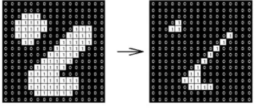
Every time we process a row we look if there’s a pixel different from zero, in that case we write in that cell the row value. Doing this we have the cells of the line memory that represent the x coordinate while the y coordinate are represented by the row value. In this manner we can take the coordinate (x,y) of the matrix of the screen, Figure B.2 on the next page shows an example.
B.3
Stereo Vision
bla bla
B.4
Calibration
bla bla
B.5
Face detection
For the edge detection part we apply the following algorithm to implement the operations of smoothing, differentiation and labeling.
B.5 Face detection 55
Appendix C
Zigbee
ZigBee protocols are intended for use in embedded applications requiring low data rates and low power consumption. ZigBee’s current focus is to define a general-purpose, inexpensive, self-organizing, mesh network that can be used for industrial control, embedded sensing, medical data collection, smoke and intruder warning, building automation, home automation, domotics, etc. The resulting network will use very small amounts of power so individual devices might run for a year or two using the originally installed battery.
C.1
Devices type
There are three different types of ZigBee device:
ZigBee coordinator(ZC): The most capable device, the coordinator forms the root of the network tree and might bridge to other networks. There is exactly one ZigBee coordinator in each network. It is able to store infor-mation about the network, including acting as the repository for security keys.
ZigBee Router (ZR): Routers can act as an intermediate router, passing data from other devices.
ZigBee End Device (ZED): Contains just enough functionality to talk to its parent node (either the coordinator or a router); it cannot relay data from other devices. It requires the least amount of memory, and therefore can be less expensive to manufacture than a ZR or ZC.
Bibliography
[1] M. H¨opken, M. Grinberg, and D. Willersinn. Modeling depth estimation errors for side looking stereo video systems. IEEE Intelligent Vehicles Symposium, 2006.
[2] V. Jeanne, F.-X. Jegaden, R. Kleihorst, A. Danilin, and B. Schueler. Real-time face detection on a dual-sensor. DSC’06, 2006.
[3] R. Kleihorst, B. Schueler, A. Danilin, and M. Heijligers. Smart camera mote with high performance vision system. DSC’06, 2006.
[4] E. Stringa and C. S. Regazzoni. Real-time video-shot detection for scene surveillance applications. IEEE Trans. Image Processing, vol. 9, pages 69–80, 2006.
[5] P. Viola and M. Jones. Rapid object detection using a boosted cascade of sim-ple features. IEEE Conference on Computer Vision and Pattern Recognition, 2001.
[6] W. Wolf, B. Ozer, and T. Lv. Smart cameras as embedded systems. Computer, vol.35, no. 9, pages 48–53, 2006.
List of Figures
1.1 Color analog monitors. . . 6 1.2 Time Lapse Recorder. . . 6 1.3 The WiCa architecture. Between the processors there is a shared
DPRAM memory. . . 8 1.4 IC3D architecture. . . 9 1.5 SIMD example. . . 10 2.1 The set up include two WiCa platforms and a central node(PC).
Every node of the network is provide by a Zigbee transceiver. . . . 14 2.2 Architecture framework . . . 15 2.3 Communication protocol between the Win32 application and the
8051 microcontroller. . . 16 2.4 Win32 application. It is the communication interface to the WiCa
devices and it gives the opportunity to run a custom application. . 17 2.5 Combo box for the commands. The picture shows the commands
supported by the two WiCa of id 70 and 202. . . 17 2.6 WiCa packet. . . 18 2.7 WiCa header. . . 18 3.1 This picture shows the interpolation process. (a) shows four
inter-ested pixels. (b) shows the vertical interpolation. (c) shows the horizontal interpolation . . . 21 3.2 This picture shows the extrapolation process. The gray pixels are
stored in the memory . . . 21 3.3 Erosion operation using a 3x3 kernel. . . 23
62 LIST OF FIGURES
3.4 The Figure shows the background subtraction algorithm with the addition of the silhouette algorithm. Figure (a) shows background + foreground. Figure (b) shows the background. Figure (c) shows the background subtraction with the silhouette algorithm . . . 24 3.5 Stereo vision with parallel axes. 3D reconstruction depends of the
solution of the correspondance problem (a); depth is estimated form the disparity of corresponding points. . . 25 3.6 (a) original image. (b) Position information provided by an edge
detector. . . 27 3.7 Image processed with a gaussian 3x3 smoothing filter and a
hori-zontal diiferentiation operation. . . 29 3.8 Image processed with a gaussian 3x3 smoothing filter and a vertical
differentiation operation. . . 30 3.9 Microcontroller interconnections. . . 31 4.1 Cameras network. . . 34 4.2 Cartesian plane and WiCa camera with position (0,0) and
orien-tation versus positive x-axis . . . 36 4.3 This example shows the Local Space of camera C1 . . . 37 4.4 This example shows the World Space after the positioning of C1
in the origin of the cartesian plane . . . 38 4.5 The figure shows that with one point, all points on the circle can
be assigned as position of the camera. . . 41 4.6 This case shows that with two points the camera can be found only
in the yellow spots. . . 41 4.7 With three points the problem is solved and it exists only one
solution shown by the yellow spot. This is the place where the camera is placed. . . 42 4.8 The figure shows the face detection algorithm running on WiCa
platforms. The white stripe on the faces shows the detection of the faces. . . 43 B.1 Silhouette algorithm. . . 55
List of Tables
4.1 Data received from smart cameras . . . 35 4.2 This example shows the localization table when the algorithm
starts, so no camera has position and orientation in the Cartesian plane yet. . . 36 4.3 map of the object’s points on the Cartesian system . . . 38