DOTTORATO DI RICERCA IN
INGEGNERIA ENERGETICA, NUCLEARE E DEL
CONTROLLO AMBIENTALE
Ciclo XXVIII
Settore Concorsuale di afferenza: 09/C2
Settore Scientifico disciplinare: ING-IND/10
Development and applications of simulation codes for
air-to-water and ground-coupled heat pump systems
Presentata da:
CLAUDIA NALDI
Coordinatore Dottorato
Relatore
Prof. Vincenzo Parenti Castelli
Prof. Enzo Zanchini
Correlatore
Prof. Gian Luca Morini
I would like to thank my supervisor Professor Enzo Zanchini and my co-advisor Professor Gian Luca Morini for their valuable help given in these three years of Doctorate.
In this Thesis, new simulation codes for the evaluation of the seasonal performance of heat pump systems are presented. The codes apply to electric air-to-water and ground-coupled heat pump systems based on a vapor compression cycle, coupled with buildings.
Heat pumps are a very efficient technology for building heating, cooling and domestic hot water (DHW) production, which reached an important development during the last decades and have been widely studied in the literature.
This work is composed of three main parts. In the first part, numerical models are developed to simulate different kinds of air-to-water heat pumps by means of the bin-method. The latter, which is derived from the European standard EN 14825 and the Italian standard UNI/TS 11300-4, is here extended in order to consider the different operating modes of mono-compressor on-off heat pumps (ON-OFF HPs), multi-compressor heat pumps (MCHPs) and inverter-driven heat pumps (IDHPs). A code for heating and DHW production mode during winter and a code for cooling and DHW production mode during summer are developed. By applying the codes, the heat pump system seasonal performance is analyzed in relation to the thermal characteristics of the building, the climate of the location and the kind of heat pump control system. The results show that the best seasonal performance in winter is obtained with IDHPs by adopting as bivalent temperature the design temperature. For reversible heat pumps used in summer for cooling and DHW production through condensation heat recovery, the primary energy saving can be higher than 30 % with respect to traditional solutions in which the heat pump supplies only cooling and DHW is produced by a gas boiler.
In the second part of this Thesis, numerical codes for the hourly simulation of air-to-water heat pump systems are developed. The dynamic codes are implemented in the software MATLAB and apply to ON-OFF HPs and to IDHPs for building heating, cooling and DHW production, coupled with storage tanks and integrated by a gas boiler or electric heaters. The codes are used, in particular, to evaluate the seasonal performance and the primary energy consumption of the multi-function inverter-driven air-to-water heat pump employed in the retrofit of a residential building in Bologna (Italy). The retrofit intervention is expected to yield a primary energy saving of more than 85 % with respect to the pre-retrofit scenario. The codes are validated by comparing the results obtained with those yielded by the dynamic software TRNSYS (maximum discrepancy 0.80 %).
The predictions of the bin-method have been proved to be in agreement with those of the dynamic simulation only in particular conditions, varying with the climate data and with the considered heat pump type. The discrepancies in the Seasonal Coefficient Of Performance (SCOP) can be higher than 20 % (ON-OFF HPs with high bivalent temperature).
(GCHP) systems is developed. The code, which employs the g-functions obtained by Zanchini and Lazzari (E. Zanchini, S. Lazzari, Energy, 59, 2013, 570-80), is implemented in MATLAB and applies to on-off and inverter-driven GCHPs, used for building heating and/or cooling. The whole system, composed by the heat pump and the coupled Borehole Heat Exchanger (BHE) field, can be simulated for several years. The code is applied to analyze the effects of the inverter and of the total length of the BHE field on the mean seasonal performance of a GCHP system designed for a residential house with dominant heating loads. The results show that 40 % increase of the BHE length can yield a SCOP enhancement of about 7 % in winter, while in summer the Seasonal Energy Efficiency Ratio (SEER) remains nearly unchanged. The replacement of the ON-OFF HP by an IDHP yields a SCOP enhancement of about 30 % and a SEER enhancement of about 52 %. The dynamic code is validated by comparing the mean monthly temperatures of the BHE fluid obtained by the proposed model with those evaluated through the software Earth Energy Designer (maximum discrepancy 2.18 %).
In questa Tesi vengono presentati nuovi codici di simulazione per la valutazione delle prestazioni stagionali di sistemi a pompa di calore. Tali codici sono riferiti a sistemi con pompe di calore elettriche aria-acqua o accoppiate al terreno, basate su un ciclo a compressione di vapore e accoppiate ad edifici.
Le pompe di calore rappresentano un’efficiente tecnologia per riscaldamento, raffrescamento e produzione di acqua calda sanitaria (ACS) negli edifici, che durante gli ultimi decenni ha raggiunto un importante sviluppo e che è stata ampiamente studiata in letteratura.
Nella prima parte di questo lavoro sono sviluppati modelli di simulazione numerica per diverse tipologie di pompe di calore aria-acqua, basati sul metodo bin. Quest’ultimo, derivato dalla norma europea EN 14825 e dalla norma italiana UNI/TS 11300-4, è qui esteso allo scopo di considerare le diverse modalità di funzionamento di pompe di calore mono-compressore on-off (ON-OFF HP), multi-compressore (MCHP) e dotate di inverter (IDHP). È sviluppato un codice per la modalità invernale di riscaldamento e produzione di ACS e un codice per la modalità estiva di raffrescamento e produzione di ACS. Impiegando i codici, le prestazioni stagionali di sistemi a pompa di calore sono analizzate in relazione alle caratteristiche termiche dell’edificio, del clima locale e del tipo di sistema di regolazione della pompa di calore. I risultati mostrano come le migliori prestazioni stagionali in inverno siano ottenute con le IDHP adottando come temperatura bivalente la temperatura esterna di progetto. Per le pompe di calore reversibili usate in estate per raffrescamento e produzione di ACS tramite recupero del calore di condensazione, il risparmio di energia primaria può superare il 30 % rispetto a soluzioni tradizionali in cui la pompa di calore provvede al solo raffrescamento e l’ACS è fornita da una caldaia a gas.
Nella seconda parte di questa Tesi sono sviluppati codici numeri per la simulazione oraria di sistemi a pompa di calore aria-acqua. I codici dinamici sono implementati sul software MATLAB e si applicano alle ON-OFF HP e IDHP per riscaldamento, raffrescamento e produzione di ACS in edifici, accoppiate a serbatoi di accumulo e integrate da una caldaia a gas o da resistenze elettriche. I codici sono utilizzati, in particolare, per valutare le prestazioni stagionali e il consumo di energia primaria della pompa di calore aria-acqua multifunzione con inverter impiegata nel retrofit di un edificio residenziale a Bologna (Italia). L’intervento di retrofit dovrebbe produrre un risparmio di energia primaria superiore all’80 % rispetto allo
dal software dinamico TRNSYS (massima differenza: 0.80 %).
Le previsioni del metodo bin si sono dimostrate in accordo con quelle della simulazione dinamica solo in particolari condizioni, al variare dei dati climatici e della tipologia di pompa di calore considerata. Le differenze nel Coefficiente di Prestazione Stagionale (SCOP) possono risultare maggiori del 20 % (ON-OFF HP con alte temperature bivalenti).
Nella terza parte di questa Tesi è sviluppato un codice di simulazione oraria per sistemi a pompa di calore accoppiata al terreno (GCHP). Il codice, che impiega le g-function ottenute da Zanchini e Lazzari (E. Zanchini, S. Lazzari, Energy, 59, 2013, 570-80), è implementato su MATLAB e si applica a GCHP on-off e con inverter, usate per riscaldamento e/o raffrescamento di edifici. L’intero sistema, composto da pompa di calore e campo di sonde geotermiche accoppiato, può essere simulato per diversi anni. Il codice è impiegato per analizzare gli effetti dell’inverter e della lunghezza totale del campo sonde sulle prestazioni stagionali medie di un sistema GCHP progettato per un edificio residenziale con carichi dominanti per riscaldamento. I risultati mostrano che un aumento della lunghezza delle sonde del 40 % può produrre in inverno un incremento di SCOP del 7 % circa, mentre in estate l’Indice di Efficienza Energetica Stagionale (SEER) rimane quasi invariato. Sostituire la ON-OFF HP con una IDHP produce un aumento di SCOP del 30 % circa e un aumento di SEER del 52 % circa. Il codice dinamico è validato confrontando le temperature medie mensili del fluido nelle sonde ottenute col modello proposto con quelle calcolate dal software Earth Energy Designer.
i
C
ONTENTS
List of Figures ... v
List of Tables ... x
Nomenclature ... xiii
Roman letters ... xiii
Greek letters ... xiv
Superscripts, subscripts ... xiv
Acronyms ... xv
1 Introduction and aim of the work ...1
2 Heat pump simulation models in the literature ...5
2.1 Heat pump design models ... 5
2.2 Temperature class models ... 6
2.2.1 Heat pump seasonal performance evaluation according to European and Italian standards ... 8
2.3 Dynamic simulation models ... 24
2.3.1 Dynamic simulation of air-to-water heat pumps with the software TRNSYS ... 27
2.4 Design and simulation of ground-coupled heat pump systems ... 33
2.4.1 The ASHRAE method ... 36
2.4.2 A recent study for ground-coupled heat pump systems design through the g-functions ... 43
2.4.3 The software Earth Energy Designer (EED) ... 48
3 Simulation codes for air-to-water heat pumps through the bin-method ... 54
3.1 Mathematical model for winter operation ... 54
ii
3.1.2 Building energy signature ... 55
3.1.3 Building domestic hot water demand ... 57
3.1.4 Heat pump characterization ... 57
3.1.5 Energy calculation for winter operation ... 60
3.2 Mathematical model for summer operation ... 64
3.2.1 Bin distribution, building energy need and heat pump characterization .... 65
3.2.2 Energy calculation for summer operation ... 67
3.3 Case studies ... 71
3.3.1 Seasonal performance of air-to-water heat pumps for heating... 71
3.3.2 Summer performance of reversible air-to-water heat pumps with heat recovery for domestic hot water production ... 79
4 Dynamic simulation codes for air-to-water heat pumps ... 84
4.1 MATLAB code for winter operation ... 84
4.1.1 Climate implementation ... 85
4.1.2 Building hourly energy need for heating ... 86
4.1.3 Building hourly energy need for domestic hot water ... 87
4.1.4 Heat pump and thermal storage characterization for winter operation .... 87
4.1.5 Hourly energy evaluations for winter operation ... 89
4.1.6 Case study ... 95
4.2 MATLAB code for summer operation ... 100
4.2.1 Climate implementation and building hourly energy needs ... 100
4.2.2 Heat pump and thermal storage characterization for summer operation 102 4.2.3 Hourly energy evaluations for summer operation ... 103
4.3 Application of the codes to the energy retrofit of a residential building in the framework of the HERB project ... 110
4.3.1 Building subject to retrofitting and energy retrofit intervention ... 110
4.3.2 Input data for the heat pump dynamic simulations ... 112
iii
4.4 Validation of the numerical codes ... 117
4.4.1 Inputs of the TRNSYS simulations... 117
4.4.2 Results and comparisons ... 121
4.5 Comparison between the simulation methods for air-to-water heat pumps .... 123
4.5.1 Implementation of the climate, building and heat pump ... 123
4.5.2 Results and discussion ... 127
5 A dynamic simulation code for ground-coupled heat pump systems ... 131
5.1 Mathematical model ... 131
5.1.1 Building and heat pump characterization ... 132
5.1.2 Borehole heat exchangers characterization ... 133
5.1.3 Calculation of the GCHP system seasonal performance ... 135
5.2 Application of the code ... 140
5.2.1 Building characteristics ... 140
5.2.2 Characteristics of the ground-coupled heat pump and of the borehole heat exchanger field ... 142
5.2.3 Analysis of the results of the simulations ... 144
5.3 Validation of the MATLAB code with the software Earth Energy Designer (EED) ... 153
6 Conclusions and future work ... 158
6.1 Conclusions ... 158
6.2 Opportunities for future work ... 160
7 Appendix ... 161
7.1 MATLAB code for air-to-water heat pumps in winter operation ... 161
7.2 MATLAB code for air-to-water heat pumps in summer operation ... 166
7.3 MATLAB code for ground-coupled heat pumps ... 174
8 Publications ... 179
8.1 International journals ... 179
iv
8.3 National journals and conferences ... 180 9 Software application ... 181 References ... 182
v
L
IST OF
F
IGURES
Figure 1.1: World annual use of primary energy by source from 1980 to 2012, data according
to EIA [1]. ... 1
Figure 1.2: Annual use of primary energy by sector in Europe, from 1990 to 2014, data according to Eurostat [3]. ... 2
Figure 1.3: Fractions of primary energy use in main sectors in Europe, in 2012, data according to Eurostat [3]... 3
Figure 2.1: Bin distribution for the heating season in the Colder climate from standard EN 14825. ... 9
Figure 2.2: Bin distribution for the heating season in the Average climate from standard EN 14825. ... 9
Figure 2.3: Bin distribution for the heating season in the Warmer climate from standard EN 14825. ... 10
Figure 2.4: Bin distribution for the cooling season from standard EN 14825. ... 10
Figure 2.5: Examples of Building Energy Signatures for heating (left) and for cooling (right). ... 11
Figure 2.6: Examples of Building Energy Signature and of characteristic curve of an air-to-water ON-OFF HP in heating mode, high temperature application, Average climate. ... 17
Figure 2.7: Examples of building energy signature and air-source heat pump characteristic curve in different operations... 24
Figure 2.8: TRNSYS Type 941 characteristics from the component proforma. ... 28
Figure 2.9: Example of heating performance file for Type 941. ... 29
Figure 2.10: Fourier – G factor graph from Ref. [39]. ... 39
Figure 2.11: G factor values and fourth order polynomial interpolating function. ... 40 Figure 2.12: Ratio between the building thermal load averaged over 4 hours and the mean daily load, during the day with maximum heating load, for a residential building
vi
in Bologna (Italy), with indoor temperature 20 °C by day and 18 °C by night
(figure from Ref. [52]). ... 43
Figure 2.13: Plots of the g-functions at r* = 0.5, for L* = 2000, 1400, 1000, 700, figure from Ref. [9]. ... 47
Figure 2.14: Discrepancy between the interpolated and the numerical values of the g-function for L* = 1000 and r* = 30, in the neighborhood of x 1 = 3.0, from Ref. [9]. ... 47
Figure 2.15: Earth Energy Design (EED) desktop. ... 48
Figure 2.16: EED input data for a double-U pipe borehole heat exchanger. ... 49
Figure 2.17: Annual trend of building heating and cooling base loads and corresponding thermal load exchanged between BHE and ground (earth base load). ... 51
Figure 2.18: Some sections of the EED output text report. ... 52
Figure 2.19: Fluid temperature profile for the last year of simulation. ... 52
Figure 2.20: Maximum and minimum fluid temperature over the simulation period. ... 53
Figure 3.1: Bin distribution for the heating season in Bologna (Italy). ... 55
Figure 3.2: Examples of trend of the winter building energy signature and characteristic curve of a mono-compressor on-off air-source heat pump. ... 56
Figure 3.3: Typical trend of the winter building energy signature and characteristic curves of a multi-compressor or an inverter-driven air-source heat pump. ... 59
Figure 3.4: Bin distribution for the cooling season in Bologna (Italy). ... 65
Figure 3.5: Typical trend of the summer building energy signature and characteristic curves of a multi-compressor or inverter-driven air-source heat pump. ... 66
Figure 3.6: Bin distribution for the heating season in Brescia, Florence and Trapani (Italy). 71 Figure 3.7: BES and characteristic curve of the ON-OFF HP. ... 72
Figure 3.8: SCOPnet and bin distribution for Brescia. ... 75
Figure 3.9: SCOPon and bin distribution for Brescia. ... 75
Figure 3.10: SCOPnet and bin distribution for Florence. ... 76
Figure 3.11: SCOPon and bin distribution for Florence. ... 76
vii Figure 3.13: SCOPon and bin distribution for Trapani. ... 77
Figure 3.14: Bin distribution for the cooling season in Palermo (Italy). ... 79 Figure 3.15: SEER with different building loads. ... 80 Figure 3.16: fcorr in cooling-only and heat recovery mode (Pdes,c = 20 kW; Eb,d,tot / Eb,c,tot = 15 %),
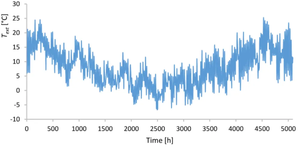
BES, bin trend. ... 81 Figure 3.17: FUE of IDHP and traditional system with different building loads. ... 82 Figure 3.18: Primary energy saving, with respect to traditional system, with different building loads. ... 83 Figure 4.1: Hourly trend of the external air temperature during the heating season in Bologna (Italy) from Meteonorm TMY. ... 85 Figure 4.2: Monthly average outdoor temperatures for the heating season in Bologna (Italy).
... 86 Figure 4.3: Plant scheme for winter operation. ... 88 Figure 4.4: Examples of curves of the COP and of the ratio ηbk,prim / ηel as functions of the
external air temperature. ... 90 Figure 4.5: Manufacturer data and interpolating function for the heat loss coefficient of the thermal storage, versus storage volume. ... 96 Figure 4.6: Building energy signature and heat pump power at Ts,h,min, for Фmax and Фmin. ... 97
Figure 4.7: Hourly trends of Text, Tbiv, Eb,h, EHP,h, Es,h, Ebk, for January 13th. ... 98
Figure 4.8: SCOPon as a function of Vs,h for different values of Tbiv, IDHP. ... 98
Figure 4.9: SCOPon as a function of Vs,h for different values of Tbiv, ON-OFF HP. ... 99
Figure 4.10: Hourly trend of the external air temperature during the cooling season in Bologna (Italy) from Meteonorm TMY. ... 101 Figure 4.11: Monthly average outdoor temperatures for the cooling season in Bologna (Italy).
... 101 Figure 4.12: Plant scheme for summer operation. ... 102 Figure 4.13: Street views of the house: Northeast side (left) and Southwest side (right). . 110 Figure 4.14: 3-D models of the house: Northeast and Northwest sides (left), Southwest and Southeast sides (right). ... 111
viii
Figure 4.15: Plans of the apartments: first floor (left), second and third floor (right). ... 111 Figure 4.16: Workspace of the TRNSYS simulations... 118 Figure 4.17: Hourly trend of COP according to TRNSYS and to the MATLAB codes, from October 1st to April 30th. ... 122 Figure 4.18: Hourly trend of EER according to TRNSYS and to the MATLAB codes, from May 1st to September 30th. ... 122 Figure 4.19: Bin profiles for Milan according to the standard UNI/TS 11300-4 and derived from the CTI’s TRY. ... 124 Figure 4.20: Bin profiles for Bologna according to the standard UNI/TS 11300-4 and derived from the CTI’s TRY. ... 124 Figure 4.21: Bin profiles for Naples according to the standard UNI/TS 11300-4 and derived from the CTI’s TRY. ... 125 Figure 4.22: Characteristic curves of the heat pumps with corresponding electric power used.
... 126 Figure 4.23: SCOP as function of Tbiv with dynamic simulation and bin simulation from CTI’s
TRY, ON-OFF HP (left) and IDHP (right), Milan. ... 127 Figure 4.24: SCOP as function of Tbiv with dynamic simulation and bin simulation from UNI/TS
11300-4, ON-OFF HP (left) and IDHP (right), Milan. ... 128 Figure 4.25: SCOP as function of Tbiv with dynamic simulation and bin simulation from UNI/TS
11300-4, ON-OFF HP (left) and IDHP (right), Bologna. ... 128 Figure 4.26: SCOP as function of Tbiv with dynamic simulation and bin simulation from UNI/TS
11300-4, ON-OFF HP (left) and IDHP (right), Naples. ... 129 Figure 4.27: Relative differences on the seasonal coefficients as functions of the bivalent temperature. ... 130 Figure 5.1: Building loads for heating and cooling-dehumidifying, from October 1st to September 30th. ... 141 Figure 5.2: Building monthly averaged loads. ... 141 Figure 5.3: BHE fluid temperature during the 10th year, L* = 700, inverter-driven heat pump.
... 144 Figure 5.4: BHE fluid maximum temperatures, L* = 700, inverter-driven heat pump. ... 144
ix
Figure 5.5: BHE fluid minimum temperatures, L* = 700, inverter-driven heat pump. ... 145
Figure 5.6: BHE fluid maximum temperatures, L* = 500, inverter-driven heat pump. ... 145
Figure 5.7: BHE fluid minimum temperatures, L* = 500, inverter-driven heat pump. ... 146
Figure 5.8: Hourly trend of Tf,m from November to January, 10th year, L* = 700. ... 147
Figure 5.9: Hourly trend of COPeff from November to January, 10th year, L* = 700. ... 148
Figure 5.10: Hourly trend of Tf,m from June to August, 10th year, L* = 700. ... 148
Figure 5.11: Hourly trend of EEReff from June to August, 10th year, L* = 700. ... 148
Figure 5.12: BHE fluid maximum temperatures, L* = 700, IDHP, monthly simulation... 149
Figure 5.13: BHE fluid minimum temperatures, L* = 700, IDHP, monthly simulation. ... 150
Figure 5.14: Yearly difference in the values of Tf,m,max, IDHP, L* = 700, monthly simulation. ... 150
Figure 5.15: Yearly difference in the values of Tf,m,min, IDHP, L* = 700, monthly simulation.151 Figure 5.16: Hourly values of the difference between Tf,m at the 5th year and Tf,m at the 10th year, IDHP, L* = 700. ... 152
Figure 5.17: Extract of the EED results. ... 154
Figure 5.18: Maximum and minimum annual values of the BHE fluid mean temperature from EED. ... 155
Figure 5.19: Annual values of Tf,m,max from the MATLAB code and from EED. ... 156
Figure 5.20: Annual values of Tf,m,min from the MATLAB code and from EED. ... 156
x
L
IST OF
T
ABLES
Table 2.1: Part load conditions for reference SCOP, air-to-water units for low temperature
applications, reference heating season Colder. ... 12
Table 2.2: Part load conditions for reference SCOP, air-to-water units for high temperature applications, reference heating season Average. ... 13
Table 2.3: Part load conditions for reference SCOP, water-to-water or brine-to-water units for medium temperature applications, reference heating season Warmer. .... 14
Table 2.4: Part load conditions for reference SEER, air-to-water units. ... 15
Table 2.5: Part load conditions for reference SEER, water-to-water or brine-to-water units. ... 15
Table 2.6: Values of the factor kσ,month. ... 20
Table 2.7: Reference conditions for performance data provided by the manufacturer. Heat pumps for heating-only or heating and DHW production. ... 21
Table 2.8: Reference conditions for performance data provided by the manufacturer. Heat pumps for DHW production only. ... 21
Table 2.9: Short circuit factor values. ... 40
Table 2.10: Temperature penalty Tp for 10 × 10 BHE field after 10 years. ... 41
Table 2.11: Tp correction factors for other BHE grid patterns. ... 41
Table 2.12: Dimensionless temperature penalty Tp* after 10 years from Ref [51]. ... 42
Table 2.13: Values of the constants x0, a6, a5, a4, a3, a2, a1, a0, and x1, b6, b5, b4, b3, b2, b1, b0, for L* = 1000. ... 46
Table 3.1: Values of the coefficients aw and bw. ... 57
Table 3.2: Heat pumps technical data. ... 72
Table 3.3: Heat pumps thermal power and COP at maximum and minimum capacity. ... 73
Table 3.4: Numerical results of some case studies. ... 74
Table 3.5: Heat pumps cooling power and EER at maximum and minimum capacity (Tw,c = 7 °C). ... 80
xi
Table 4.1: Hourly load coefficients for domestic hot water in residential buildings. ... 87
Table 4.2: Heat pump power [kW] at the minimum and maximum temperature of the storage. ... 96
Table 4.3: Heat pump COP at the minimum and maximum temperature of the storage. .... 97
Table 4.4: Heat pump power [kW] and (COP) in heating mode; Ts,h = 40 °C. ... 113
Table 4.5: Heat pump power [kW] and (COP) in heating mode; Ts,h = 38 °C. ... 114
Table 4.6: Heat pump power [kW] and (COP) in DHW mode; Ts,d = 50 °C. ... 114
Table 4.7: Heat pump power [kW] and (EER) in cooling-only mode; Ts,c = 7 °C... 115
Table 4.8: Heat pump power [kW] and (EER) in cooling-only mode; Ts,c = 5 °C... 115
Table 4.9: Heat pump power [kW] and (EER) in heat recovery mode; Ts,c = 7 °C. ... 115
Table 4.10: Heat pump power [kW] and (EER) in heat recovery mode; Ts,c = 5 °C. ... 115
Table 4.11: Annual electric energy use and corresponding primary energy consumption. 116 Table 4.12: Heat pump performance inputs in heating mode for Type 941 of TRNSYS. ... 119
Table 4.13: Heat pump performance inputs in cooling-only mode for Type 941 of TRNSYS. ... 119
Table 4.14: Seasonal performance coefficients obtained with TRNSYS and with the MATLAB codes. ... 121
Table 4.15: IDHP power [kW] and (COP) for different inverter frequencies and external air temperatures. ... 126
Table 5.1: Values of the constants x0, a6, a5, a4, a3, a2, a1, a0, and x1, b6, b5, b4, b3, b2, b1, b0, for L* = 500. ... 134
Table 5.2: Values of the constants x0, a6, a5, a4, a3, a2, a1, a0, and x1, b6, b5, b4, b3, b2, b1, b0, for L* = 700. ... 135
Table 5.3: Heat pump power [kW] and (COP) in heating mode; Tw,h = 40 °C. ... 142
Table 5.4: Heat pump power [kW] and (EER) in heating mode; Tw,c = 7 °C. ... 143
Table 5.5: SCOP values with or without inverter, L* equal to 500 or 700, 10th year. ... 146
Table 5.6: SEER values with or without inverter, L* equal to 500 or 700, 10th year. ... 147
Table 5.7: SCOP values with or without inverter, L* equal to 500 or 700, 50th year. ... 152
xii
xiii
N
OMENCLATURE
R
OMAN LETTERS
A Dimensionless load amplitude bu Temperature reduction factor Cc Degradation coefficient
cp Specific heat capacity at constant pressure
D Diameter
E Energy
Fsc Short Circuit Factor
Fo Fourier number
G G factor
g g-function
H Solar radiation
i i-th bin or hour
k Thermal conductivity
L Borehole length
M Number of inverter frequencies
ṁ Mass flow rate
N Number of compressors
n Number of activated compressors
P Power
pd Load coefficient for domestic hot water
Q Thermal energy
q Thermal load per unit length R Thermal resistance per unit length
r Radial coordinate
S Floor area
T Temperature
t Time
xiv
V Volume
V̇ Volumetric flow rate
z Vertical coordinate
G
REEK LETTERS
α Thermal diffusivity η Efficiency ρ Density σ Standard deviation Ф Inverter frequencyS
UPERSCRIPTS
,
SUBSCRIPTS
* Dimensionless quantity avail Available b Building bin Bin biv Bivalent bk Back-up c Cooling compr Compressor cond Condenser corr Correctiond Domestic hot water
des Design despr Desuperheater dis Distribution dly Daily eff Effective el Electric em Emission
xv
evap Evaporator
ext External air
f Fluid g Ground h Heating HP Heat pump in Inlet int Internal m Mean max Maximum min Minimum mly Monthly
net Of the heat pump
on Of the heat pump and back-up system
out Outlet
p Penalty
prim Primary
r Condensation heat recovery
res Residual s Storage tot Total uncov Uncovered us Used virt Virtual w Water yly Annual zl Zero-load
A
CRONYMS
BES Building Energy Signature
BHE Borehole Heat Exchanger
COP Coefficient Of Performance
xvi
DHW Domestic Hot Water
DST Duct STorage
EER Energy Efficiency Ratio
FCS Finite Cylindrical Source
FLS Finite Line Source
FUE Fuel Utilization Efficiency
GCHP Ground-Coupled Heat Pump
ICS Infinite Cylindrical Source
IDHP Inverter-Driven Heat Pump
ILS Infinite Line Source
MCHP Multi-Compressor Heat Pump
ON-OFF HP Mono-compressor ON-OFF Heat Pump
PLF Partial Load Factor
SCOP Seasonal Coefficient Of Performance
SEER Seasonal Energy Efficiency Ratio
SPF Seasonal Performance Factor
TMY Typical Meteorological Year
TOL Temperature Operative Limit
1
1
I
NTRODUCTION AND AIM OF THE
WORK
The economic growth of the 20th century has been based on a progressive increase of the world annual use of fossil fuels. The world annual use of primary energy is still increasing and fossil fuels represent even now the most important source of primary energy, as shown in Figure 1.1. The figure illustrates the world annual use of primary energy by source from 1980 to 2012, according to EIA [1] (US Energy Information Administration).
Figure 1.1: World annual use of primary energy by source from 1980 to 2012, data according to EIA [1].
As evidenced by Figure 1.1, 86 % of the world primary energy use in 2012 is due to oil, carbon and gas. The fossil-fuel-based development has caused two important problems: the
0 100 200 300 400 500 600 1980 1985 1990 1995 2000 2005 2010 other gas coal oil EJ year
2
reserves of oil and natural gas are decreasing and the emission of carbon dioxide and of other greenhouse gases is causing a climate change (see Ref. [2]). As a consequence, all the industrialized and developing countries and, most of all, the European Union, are struggling to shift the economic growth towards a sustainable development, based on two main pillars: the increase of energy efficiency and the use of renewable energy sources.
The energy policy of the European Union already obtained some success: the annual use of primary energy of the Union is slightly decreasing from 2006, as shown in Figure 1.2, which illustrates the use of primary energy of the European Union by sector from 1990 to 2014, according to Eurostat [3] (European Commission portal for statistics).
Figure 1.2: Annual use of primary energy by sector in Europe, from 1990 to 2014, data according to Eurostat [3].
Figure 1.2 reveals that the fractions of energy use in the residential sector and in the service sector are quite relevant. The fractions of primary energy use in sectors for 2014 are better evidenced by Figure 1.3, where it is shown that the sum of the fractions which refer to the residential sector and to the service sector (i.e., the total fraction due mainly to building operation) is 38.1 %. 0 10 20 30 40 50 60 1990 1992 1994 1996 1998 2000 2002 2004 2006 2008 2010 2012 2014 Other Agricolture Services Residential Transport Industry EJ year
3 Figure 1.3: Fractions of primary energy use in main sectors in Europe, in 2012, data according to
Eurostat [3].
According to an official document of the European Commission [4], buildings use 40 % of the total European energy consumption and generate 36 % of greenhouse gases in Europe. As a consequence, important steps towards the reduction of the use of fossil fuels in Europe would be the enhancement of the energy efficiency of buildings and the use of renewable energy sources in building plants. In particular, the European Commission has enacted the EPBD Recast Directive [5], which promotes in the Member States a transition to Nearly Zero Energy Buildings (namely buildings with very low energy needs) within 2020. In the Directive [5], the improvement of the thermal performance of the building envelope and the improvement of the heating, cooling and ventilating systems are recommended.
Heat pump systems represent useful solutions for building air-conditioning and Domestic Hot Water (DHW) production, which reached an important development during the last decades ([6], [7]). Heat pumps can contribute to achieve the mentioned European objectives, since aero-thermal, geothermal and hydrothermal energy are recognized as renewable energy sources by the European RES Directive [8].
Thanks to the relative cheapness of the plant, air-source heat pumps are good candidates for the replacement or integration of gas boilers in retrofits of existing buildings. Ground-Coupled Heat Pumps (GCHPs) achieve better performance, but require higher investment costs and soil drilling. Consequently, they are at present less widely used. A heat pump performance is strongly influenced by the variable heat load of the building, kind of control system and source temperature. Therefore, the calculation of the seasonal performance is not an easy task. In this Thesis, new simulation codes are developed for the
0.259 0.332 0.248 0.133 0.022 0.006 Industry Transport Residential Services Agricolture Other
4
evaluation of the seasonal performance of air-to-water and ground-coupled heat pump systems for building heating, cooling and DHW production.
The evaluation of a heat pump seasonal efficiency has been widely investigated in the literature; Chapter 2 of this Thesis provides a classification of the available methods, and stresses the differences between those methods and the new simulation models proposed. Chapter 3 presents new mathematical codes for the simulation of air-to-water heat pumps through the bin-method. Different calculation methods are employed for mono-compressor on-off heat pumps (ON-OFF HPs), multi-compressor heat pumps (MCHPs) and inverter-driven heat pumps (IDHPs). By applying the codes, the seasonal efficiency of heat pump systems is analyzed in relation to the characteristics of the building, local climate and kind of heat pump control system.
In Chapter 4, new codes for the hourly simulation of air-to-water heat pump systems are presented. The dynamic code developed for winter operation is used to analyze the seasonal performance of heat pump heating systems as a function of the bivalent temperature and of the volume of the thermal storage tank. Moreover, the dynamic codes are used to calculate the primary energy consumption of the IDHP used in the retrofit of a residential building in Bologna (North-Center Italy).
Chapter 5 presents a new code for the hourly simulation of ground-coupled heat pump systems. The code employs the g-functions obtained by Zanchini and Lazzari [9] and is applied to analyze the effects of the inverter and of the total length of the BHE field on the seasonal efficiency of a GCHP system designed for heating and cooling a residential house with dominant heating loads.
Chapter 6 reports the conclusions of this Thesis and some opportunities for future work. The developed codes are shown in the Appendix, while the publications and a software application derived from the work of this Thesis appear in Chapters 8 and 9, respectively.
5
2
H
EAT PUMP SIMULATION MODELS IN
THE LITERATURE
In this chapter, a classification of the methods for the simulation of heat pump systems is presented. Design models, temperature class approaches and dynamic simulation methods are described and compared to each other. In particular, the heat pump simulation methods indicated by the European standard EN 14825 [10] and the Italian standard UNI/TS 11300-4 [11] are analyzed. The dynamic simulation of air-to-water heat pumps by means of the software TRNSYS is also described.
Some design methods of borehole heat exchanger fields for ground-coupled heat pump systems are studied too. The ASHRAE method, models based on the g-functions and the software Earth Energy Designer are particularly analyzed.
2.1 H
EAT PUMP DESIGN MODELS
Several approaches for a heat pump simulation are available in the literature. As noticed by Afjei and Dott [12], the different models can be classified on the basis of the level of detail of the calculations, aim of the model and computational time required to run it.
There exist models for a heat pump design, whose aim is to optimize the heat pump unit on the level of the refrigerant cycle. These models require high computational time and represent each heat pump component individually, in order to optimize the interaction between the evaporator, the compressor, the condenser and the expansion valve.
Most of these models are empirical and rely both on physical equations and on numerical correlations derived from experimental results ([13]-[15]); fewer models are based on CFD simulations.
6
2.2 T
EMPERATURE CLASS MODELS
Other simulation models focus on the whole heat pump system. With this approach the heat pump is a black box with given performance (at fixed source and sink temperatures), coupled to a building in a specific climate, and possibly provided with a thermal storage tank and a back-up system. In this case, the aim is to simulate the entire system and to optimize its seasonal performance.
Some of these models are based on a temperature class approach, like the methods indicated by the European standard EN 14825 [10] and by the Italian standard UNI/TS 11300-4 [11], which simulate a heat pump behavior with the bin-method. As will be explained in detail in Subsection 2.2.1, a bin represents the number of hours, in a selected time period, with approximately the same value of external air temperature. A selected climate is thus schematized by means of a bin trend, which gives the local distribution of outdoor temperature.
Frequently, comparisons between different commercial heat pumps refers to the Coefficient Of Performance, COP (ratio between the thermal power released and the corresponding electric power used, in heating or DHW production mode) or to the Energy Efficiency Ratio, EER (ratio between the cooling power released and the corresponding electric power used, in cooling mode) of single operating conditions. In this case, the COP or EER is measured at specific temperatures of the heat pump source and sink, according to the European standards EN 14511-2 [16] and EN 14511-3 [17]. With this method, however, only approximate comparisons for selected conditions can be made, but no estimations of a heat pump seasonal efficiency can be performed. The models indicated by the standards [10], [11], on the contrary, are able to give predictions about a heat pump seasonal performance (Seasonal Coefficient Of Performance, SCOP, and Seasonal Energy Efficiency Ratio, SEER), by weighting the COP or EER obtained in each bin on the basis of its duration.
Cecchinato et al. [18], for instance, evaluated the performance of vapor compression heat pumps by means of a simplified numerical method, based on performance data at nominal conditions and on refrigerant circuit information. By solving a system of equations, the method estimates the heat pump cooling or heating capacity and power consumption at part load conditions for mono-compressor on-off, bi-compressor and inverter-driven heat pumps. The authors applied the method to evaluate, in four test conditions, the EER at full load and at part load of two reversible air-to-water heat pumps (a mono-compressor on-off heat pump and an inverter-driven heat pump). Hence, they evaluated the SEER of the systems through a simple temperature class approach, by employing the weighted average of the EER values
7 obtained in the four test conditions. This method refers to a preliminary version of the standard EN 14825 [10], where weighting coefficients representing conventional operating times were provided for each of the four test conditions, as functions of the heat pump typology. The so-obtained seasonal performance coefficient can be used as a reference for energy comparisons between different heat pumps, or for a first approximate evaluation of the system energy consumption when detailed information about the building energy demand is not available. The authors obtained a good agreement between the predicted SEER values and the experimental results.
Kinab et al. [15] employed a similar method to evaluate the seasonal performance of an air-to-water heat pump in heating mode and in cooling mode. The authors developed a model able to evaluate the heat pump performance for several system configurations by means of detailed sub-models for each heat pump component (heat pump design model). The heat pump model was coupled to a model for building energy simulation, in order to calculate the system seasonal performance parameters, SCOP and SEER. The heat pump model provides the values of COP or EER for different conditions of part load and outdoor temperature, while the building model provides the corresponding weighting coefficients. In this case, the weighting coefficient is evaluated as the fraction of energy which the system delivers in a specific condition of part load and outdoor temperature over the total energy delivered to the building.
Francisco et al. [19] adopted a different simulation strategy, by employing computer modeling in which the bin-method described by ASHRAE [20] is implemented in order to investigate the influence of the climate on the seasonal efficiency of air-to-air heat pumps in heating mode. The authors evaluated the system performance in each bin through a simulation model which includes the effects of the back-up system (electric heaters) and of the duct losses. The energy consumption of the heat pump obtained in each bin was multiplied by the number of hours of the bin and then summed to get seasonal results. The authors considered two climates of the Northwest United States and found that a heat pump seasonal energy consumption is strongly affected by the climate, by the heat pump control strategy and by the duct losses. Some common control strategies that employ great use of back-up heat, in particular, can seriously compromise the expected heat pump seasonal performance, especially if combined with important duct losses.
Sarbu et al. [21] developed a computational model for the calculation of the seasonal energy performance of air-to-water heat pumps employed to provide building heating and domestic hot water production. The model is based on the bin-method defined in the European standard EN 15316-4-2 [22] and allows the evaluation of a heat pump SCOP (called in the
8
standard [22] SPF, namely Seasonal Performance Factor). The authors performed a comparative analysis of different building heating solutions, investigating the economic, energy and environmental advantages of employing heat pumps as heating generation systems.
The models based on a temperature class approach have a medium level of detail (e.g. they cannot consider the charge and discharge of a thermal storage tank coupled to a heat pump), but they are easy to use, do not require long computational time and can yield accurate predictions about the seasonal behavior of a heat pump system. In addition, they can be used for fast comparisons, in terms of seasonal efficiency, between different heat pump devices or between different heat generation technologies.
2.2.1 Heat pump seasonal performance evaluation according to European and Italian
standards
The European standard EN 14825 [10] and the Italian standard UNI/TS 11300-4 [11] present calculation methods for the evaluation of the seasonal performance of heat pumps in heating, cooling and DHW production mode. The standards [10], [11] suggest to model the outdoor climate by means of the bin-method. A bin represents the number of hours, during a selected time period, in which the external air has a value of temperature within a fixed interval, centered on an integer value of temperature and 1 K wide. For instance, a bin duration of 20 hours in correspondence of an outdoor temperature Text equal to 15 °C means that for 20
hours during a certain time period the external air temperature had a value between 14.5 °C and 15.5 °C.
The standard EN 14825 [10] gives indication to calculate the reference Seasonal Coefficient Of Performance (SCOP) of heat pumps in heating mode and the reference Seasonal Energy Efficiency Ratio (SEER) of heat pumps in cooling mode.
The standard [10] splits Europe in three winter climates (Colder, Average and Warmer) and directly assigns the bin trends for the reference heating season of each climate. The duration of each bin is rounded to a whole number and is derived from weather data collected over the 1982 – 1999 period for the locations of Helsinki, Strasbourg and Athens, selected as representative of the Colder, Average and Warmer climate, respectively.
Figures 2.1-2.3 show the bin profiles of the Colder, Average and Warmer heating seasons derived from Ref. [10].
For selected heat pump and building, one can calculate a value of Seasonal Coefficient Of Performance for each of the three reference climate and compare different heat pump models under the same reference conditions.
9 Figure 2.1: Bin distribution for the heating season in the Colder climate from standard EN 14825.
Figure 2.2: Bin distribution for the heating season in the Average climate from standard EN 14825. 0 50 100 150 200 250 300 350 400 -10 -9 -8 -7 -6 -5 -4 -3 -2 -1 0 1 2 3 4 5 6 7 8 9 10 11 12 13 14 15 b in [h] Text[°C] Heating season Average climate 0 50 100 150 200 250 300 350 400 450 500 550 600 -24 -22 -20 -18 -16 -14 -12 -10 -8 -6 -4 -2 0 2 4 6 8 10 12 14 b in [h] Text[°C] Heating season Colder climate
10
Figure 2.3: Bin distribution for the heating season in the Warmer climate from standard EN 14825.
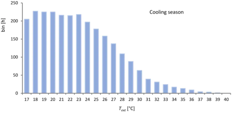
Regarding the cooling season, the standard [10] suggest a single bin profile for whole Europe, illustrated in Figure 2.4.
Figure 2.4: Bin distribution for the cooling season from standard EN 14825.
It can be noticed from Figures 2.1-2.4 that the bin trends of the standard [10] are stopped in correspondence of an outdoor temperature equal to 16 °C for all climates in cooling and heating mode. In the standard [10], in fact, the heat pump is considered coupled to a building whose loads are expressed as a linear function of the external air temperature, Text. The
method for the determination of this function, called Building Energy Signature (BES), is described in the European standard EN 15603 [23]. The standard EN 14825 [10] considers BES lines which vanishes for Text equal to 16 °C (in this Thesis called zero-load external air
temperature, Tzl). In Figure 2.5, examples of linear BES lines for heating and for cooling are
shown. 0 50 100 150 200 250 17 18 19 20 21 22 23 24 25 26 27 28 29 30 31 32 33 34 35 36 37 38 39 40 b in [h] Text[°C] Cooling season 0 50 100 150 200 250 300 350 400 450 500 550 0 1 2 3 4 5 6 7 8 9 10 11 12 13 14 15 b in [h] Text[°C] Heating season Warmer climate
11 Figure 2.5: Examples of Building Energy Signatures for heating (left) and for cooling (right).
In Figure 2.5, Pdes is the design load, namely the building load in correspondence of the
outdoor design temperature, Tdes. With reference to the heating mode, the standard [10] sets
the outdoor design temperature, Tdes,h, equal to -22 °C for the Colder climate, -10 °C for the
Average climate and 2 °C for the Warmer climate; the outdoor design temperature for cooling, Tdes,c, is 35 °C. It can be noticed that, while the values of Tdes,h for the winter climates
coincide with the minimum outdoor temperature obtainable from the bin trends, the summer bin profile presents values of Text greater than the summer outdoor design
temperature.
The standard [10] sets the part load conditions at which the heat pump COP or EER must be evaluated by the manufacturer, in order to be used as input data for the calculation of the reference seasonal performance coefficients. Indications are given for testing the heat pumps at part load conditions and for measuring their performance, with reference to the European standards EN 14511-2 [16] and EN 14511-3 [17].
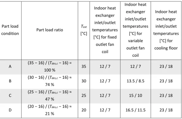
Ref. [10] differentiates the part load conditions on the basis of the heat pump typology (air-to-air, air-to-water etc.) and, referring to the heating mode, also on the basis of the indoor heat exchanger temperature (low, medium, high and very high) and on the climate (Colder, Average, Warmer). Table 2.1 reports the part load conditions A–G at which an air-to-water heat pump for low temperature applications must be tested in order to determine the reference SCOP in the Colder climate.
0 10 20 30 40 50 -12 -8 -4 0 4 8 12 16 20 24 28 32 36 40 P [kW ] Text[ C] Pdes,h Tdes,h Tzl Heating Cooling Tdes,c Pdes,c
12
Table 2.1: Part load conditions for reference SCOP, air-to-water units for low temperature applications, reference heating season Colder.
Part load
condition Part load ratio
Text [°C] Indoor heat exchanger inlet/outlet temperatures [°C] for fixed outlet units
Indoor heat exchanger inlet/outlet temperatures [°C] for variable outlet
units A (-7− 16) / (Tdes,h− 16) ≈ 61 % -7 30 / 35 25 / 30
B (2− 16) / (Tdes,h− 16) ≈ 37 % 2 30 / 35 22 / 27
C (7− 16) / (Tdes,h− 16) ≈ 24 % 7 30 / 35 20 / 25
D (12− 16) / (Tdes,h− 16) ≈ 11 % 12 30 / 35 19 / 24
E (TOL− 16) / (Tdes,h− 16) TOL 30 / 35
interpolation or extrapolation from the temperatures closest to
TOL
F (Tbiv− 16) / (Tdes,h− 16) Tbiv 30 / 35
Interpolation between the upper and lower temperatures closest to
Tbiv
G (-15− 16) / (Tdes,h− 16) ≈
82 % -15 30 / 35 27 / 32
In Table 2.1, the part load ratio gives, for each of the A–G conditions, the percentage of the building design load at which the heat pump must be tested. It is possible to calculate the seasonal performance coefficients of a heat pump for more than one Pdes value.
In Table 2.1, TOL is the Temperature Operative Limit, namely the minimum value of Text, given
by the heat pump manufacturer, at which the heat pump is able to deliver heating capacity. Tbiv is the bivalent temperature, namely the outdoor temperature at which the heat pump
capacity equals the building load. These temperature values vary from case to case; the European standard [10], however, indicates to use bivalent temperatures equal to or lower than -7 °C for the Colder climate, equal to or lower than 2 °C for the Average climate and equal to or lower than 7 °C for the Warmer climate.
The part load condition G is applied in case of Colder climate if the TOL is lower than -20 °C. For each part load condition, the inlet and outlet temperatures of the indoor heat exchanger are differentiated between fixed and variable outlet heat pumps. The second heat pump typology, which will not be analyzed in this Thesis, allows a variation of the indoor heat exchanger outlet temperature as a function of the external air temperature.
13 Table 2.2 shows the part load conditions A–F at which an air-to-water heat pump for high temperature applications must be tested in order to determine the reference SCOP in the Average climate according to the standard [10].
Table 2.2: Part load conditions for reference SCOP, air-to-water units for high temperature applications, reference heating season Average.
Part load
condition Part load ratio
Text [°C] Indoor heat exchanger inlet/outlet temperatures [°C] for fixed outlet units
Indoor heat exchanger inlet/outlet temperatures [°C] for variable outlet
units A (-7− 16) / (Tdes,h− 16) ≈ 88 % -7 47 / 55 44 / 52
B (2− 16) / (Tdes,h− 16) ≈ 54 % 2 47 / 55 34 / 42
C (7− 16) / (Tdes,h− 16) ≈ 35 % 7 47 / 55 28 / 36
D (12− 16) / (Tdes,h− 16) ≈ 15 % 12 47 / 55 22 / 30
E (TOL− 16) / (Tdes,h− 16) TOL 47 / 55
interpolation or extrapolation from the temperatures closest to
TOL
F (Tbiv− 16) / (Tdes,h− 16) Tbiv 47 / 55
Interpolation between the upper and lower temperatures closest to
Tbiv
From Table 2.2 one can note that the part load condition G, which refers to Text equal to -15 °C,
does not apply to the case of Average climate, whose minimum outdoor temperature is Tdes,h = -10 °C. In addition, if the TOL declared by the manufacturer is lower than Tdes,h of the
considered climate, it may be assumed equal to Tdes,h.
Table 2.3 reports the part load conditions for a water-to-water heat pump, or a brine-to-water heat pump, for medium temperature heating applications in the Warmer climate.
14
Table 2.3: Part load conditions for reference SCOP, water-to-water or brine-to-water units for medium temperature applications, reference heating season Warmer.
Part load
condition Part load ratio
Ground water inlet temperature [°C] Brine inlet temperature [°C] Indoor heat exchanger inlet/outlet temperatures [°C] for fixed outlet units Indoor heat exchanger inlet/outlet temperatures [°C] for variable outlet units B (2− 16) / (Tdes,h− 16) = 100 % 10 0 40 / 45 40 / 45 C (7− 16) / (Tdes,h− 16) ≈ 64 % 10 0 40 / 45 34 / 39 D (12− 16) / (Tdes,h− 16) ≈ 29 % 10 0 40 / 45 26 / 31 F (Tbiv − 16) / (Tdes,h − 16) 10 0 40 / 45 Interpolation between upper and lower temperatures closest to Tbiv
From Table 2.3 one can note that the part load condition A (which refers to Text = -7 °C) does
not apply to the case of Warmer climate, whose minimum outdoor temperature is Tdes,h = 2 °C.
The part load condition E refers to Text = Tdes,h in the cases of water-to-water or brine-to-water
heat pumps, therefore in the Warmer climate the condition E equals the condition B. Tables 2.4, 2.5 show the part load conditions for the determination of the reference SEER of air-to-water heat pumps and water-to-water (or brine-to-water) heat pumps, respectively. In part load condition A (full load), the heat pump power is considered equal to the building cooling load, which means that the bivalent temperature for the cooling mode is 35 °C.
15 Table 2.4: Part load conditions for reference SEER, air-to-water units.
Part load
condition Part load ratio
Text [°C] Indoor heat exchanger inlet/outlet temperatures [°C] for fixed outlet fan coil Indoor heat exchanger inlet/outlet temperatures [°C] for variable outlet fan coil Indoor heat exchanger inlet/outlet temperatures [°C] for cooling floor A (35− 16) / (Tdes,c− 16) = 100 % 35 12 / 7 12 / 7 23 / 18 B (30− 16) / (Tdes,c− 16) ≈ 74 % 30 12 / 7 13.5 / 8.5 23 / 18 C (25− 16) / (Tdes,c− 16) ≈ 47 % 25 12 / 7 15 / 10 23 / 18 D (20− 16) / (Tdes,c− 16) ≈ 21 % 20 12 / 7 16.5 / 11.5 23 / 18
Table 2.5: Part load conditions for reference SEER, water-to-water or brine-to-water units.
Part load conditio
n
Part load ratio
Outdoor heat exchanger inlet/outlet temperatures
[°C]
Indoor heat exchanger inlet/outlet temperatures [°C] Cooling tower Ground coupled applicatio n Dry coole r Fixed outlet fan coil Variable outlet fan coil Cooling floor A (35− 16) / (Tdes,c− 16) = 100 % 30 / 35 10 / 15 50 / 55 12 / 7 12 / 7 23 / 18 B (30− 16) / (Tdes,c− 16) ≈ 74 % 26 / 31 10 / 15 45 / 50 12 / 7 13.5 / 8.5 23 / 18 C (25− 16) / (Tdes,c− 16) ≈ 47 % 22 / 27 10 / 15 40 / 45 12 / 7 15 / 10 23 / 18 D (20− 16) / (Tdes,c− 16) ≈ 21 % 18 / 23 10 / 15 35 / 40 12 / 7 16.5 / 11.5 23 / 18
16
The standard [10] requires the determination of a heat pump power, COP and EER in correspondence of the bins representative of the predefined part load conditions. If for a condition the heat pump power at full load is equal to or lower than the required building load, the corresponding power, COP and EER values at full load must be used. If the heat pump power at full load is higher than the required building load, the heat pump performance must be calculated depending on the capacity control of the unit. In particular, mono-compressor on-off heat pumps employ on-off cycles to match the building needs. As evidenced by Henderson et al. [24], on-off cycles cause an efficiency loss of the heat pump, since the electric energy consumption of the unit does not vanish during the off-cycle and, when the heat pump restarts, its compressor has to re-establish the pressure.
The efficiency loss due to on-off cycles is taken into account by Ref. [10] through the correction factor, fcorr. The factor fcorr, evaluated for air-to-water, water-to-water and
brine-to-water heat pumps according to Eq. (2.1), multiplies the heat pump COP or EER at full load in order to derive the corresponding part load value.
( ) ( ) ( ) 1 corr c c CR i f i C CR i C . (2.1)In Eq. (2.1), the letter i indicates the i-th predefined part load condition, CR is the capacity ratio and Cc is the degradation coefficient. The capacity ratio CR is the ratio between the
building load and the heat pump power at the same temperature conditions. If the heat pump power equals the building demand, CR is equal to 1 and the correction factor for on-off condition turns out equal to 1. The degradation coefficient Cc measures the specific heat
pump efficiency decrease for on-off cycles and should be determined for each specific unit by means of laboratory tests. If Cc is not determined by tests, then the default value of 0.9
shall be used.
Multi-compressor and inverter-driven heat pumps, on the contrary, are able to adapt the power released in order to follow the building load and delay the on-off cycles activation. In these cases, the standard [10] indicates to determine the heat pump power, COP and EER at the step of the heat pump capacity closest to the required building load. If this step does not allow to reach the building load within ±10 % (e.g. between 8.1 kW and 9.9 kW for a required building load of 9 kW), then the heat pump performance must be evaluated at the steps on either side of the required building load. The part load heat pump power, COP and EER are then determined by linear interpolation between the results obtained from these two steps. If the smallest control step of the unit is higher than the required building load, the procedure for mono-compressor on-off heat pumps shall apply.
17 The European standard [10] evaluates the heat pump power and COP (or EER) in each bin through linear interpolations between the values of the two closest part load conditions. Regarding the heating mode, the heat pump performance for values of Text above the part
load condition D is extrapolated from the values at the part load conditions C and D. Regarding the cooling mode, for values of Text above the part load condition A or below the
part load condition D, the same heat pump performance in correspondence of the condition A or of the condition D is used, respectively.
Figure 2.6 shows an example of winter BES and of characteristic curve of an air-to-water ON-OFF HP for high temperature application in the Average climate, where the heat pump power has been obtained by interpolating the values at the part load conditions A–F, according to Ref. [10].
Figure 2.6: Examples of Building Energy Signature and of characteristic curve of an air-to-water ON-OFF HP in heating mode, high temperature application, Average climate.
In Figure 2.6 one can note the balance point, which is the intersection between the BES and the heat pump characteristic curve at full load. The outdoor temperature corresponding to the balance point is called bivalent temperature, Tbiv. As previously mentioned, at Tbiv the
heat pump power equals the building load. Considering the heating mode, for values of Text
between the TOL and Tbiv the heat pump power is lower than the building need and an
additional back-up system is necessary to fulfil the full heating load. The standard [10] considers as back-up system only electric heaters, whereas the codes developed in this Thesis for the evaluation of a heat pump seasonal efficiency distinguish between electric heaters and gas boiler. For values of Text higher than Tbiv, the heat pump power at full load is higher
0 10 20 30 40 50 60 70 -10 -9 -8 -7 -6 -5 -4 -3 -2 -1 0 1 2 3 4 5 6 7 8 9 10 11 12 13 14 15 16 P [kW ] Text[ C] BES ON-OFF HP Tbiv A B C D E F TOL = Tdes,h
18
than the heating demand and the heat pump COP must be corrected as previously described. For values of Text lower than the TOL, the heat pump is not running and only the back-up
system is activated.
Considering the cooling mode, the heat pump power at full load is higher than the building demand for values of Text below Tbiv, whereas for outdoor temperatures above Tbiv the heat
pump is not able to completely satisfy the cooling load, but no back-up systems are employed. The European standard [10] takes into account the real COP (or EER) values of a heat pump only for a limited number of predefined conditions, among which linear interpolations are employed. With this method, however, considerable approximations are introduced, especially for multi-compressor heat pumps (MCHPs) and inverter-driven heat pumps (IDHPs), in correspondence of the bins intermediate between two part load conditions. The codes developed in this Thesis, on the contrary, calculate the COP (or EER) values for each bin, by using for MCHPs and IDHPs a number of characteristic curves corresponding to different heat pump capacity (see Chapter 3).
Different reference seasonal coefficients are defined by the standard EN 14825 [10]. The Seasonal Coefficient Of Performance of the heat pump, SCOPnet, is the ratio between the
thermal energy delivered by the heat pump during the heating season and the corresponding electric energy used. SCOPnet is evaluated by Ref. [10] as:
, 1 , 1 ( ) ( ) ( ) ( ) ( ) ( ) ( ) n bin b h bk i net n b h bk bin i t i P i P i SCOP P i P i t i COP i
. (2.2)In Eq. (2.2), i indicates the i-th bin, n is the total amount of bins for the selected winter climate, tbin (i) is the time duration of the i-th bin, Pb,h (i) is the thermal power required by the building
in the i-th bin (obtainable from the BES multiplying Pdes,h by the part load ratio of the i-th bin), Pbk (i) is the power released by the electric back-up system in the i-th bin and COP (i) is the
value of Coefficient Of Performance obtained for the i-th bin.
Obviously, the difference between Pb,h and Pbk, employed by Ref. [10] to evaluate the SCOPnet
value, is equal to the thermal power delivered by the heat pump. The energy supplied and used by the back-up system, in fact, does not apply for the calculation of SCOPnet, which refers
only to the heat pump.
Another performance coefficient for the heating season is the Seasonal Coefficient Of Performance of the whole system (composed of heat pump and back-up system), SCOPon,
19 the heat pump and, if needed, by the back-up system) and the total electric energy used by the system: , 1 , 1 ( ) ( ) ( ) ( ) ( ) ( ) ( ) n bin b h i on n b h bk bin bk i t i P i SCOP P i P i t i P i COP i
. (2.3)The thermal power that the back-up electric heaters give is obviously equal to the electric power that they use and both these quantities are indicated as Pbk in Eq. (2.3).
No back-up systems are present for the heat pump cooling mode and only the seasonal coefficient SEERon is defined:
, 1 , 1 ( ) ( ) ( ) ( ) ( ) n bin b c i on n b c bin i t i P i SEER P i t i EER i
, (2.4)where Pb,c (i) is the cooling power required by the building in the i-th bin (obtainable from the
BES multiplying Pdes,c by the part load ratio of the i-th bin) and EER (i) is the value of Energy
Efficiency Ratio obtained for the i-th bin.
In Eq. (2.4), using Pb,c instead of the heat pump power yields a small approximation due to
the bins with temperature higher than Tbiv (35 °C), where the whole building demand is not
covered by the heat pump.
Both SCOPnet, SCOPon and SEERon refer to the active mode of a heat pump, namely to the hours
in which the building load is present and the heating or cooling function of the heat pump is thus activated. Energy consumptions can occur also when the heat pump is not used to fulfil the building demand, such as the energy consumption of the crankcase heater or of the standby mode of the unit (mode wherein the unit is partially switched off and can be reactivated by a control device or timer). These consumptions, which are considered by the standard [10] with the definition of other seasonal coefficients, are not studied in the present Thesis.
The Italian standard UNI/TS 11300-4 [11] defines a calculation method to evaluate the primary energy consumption of a heat pump system for building heating and/or domestic hot water production. According to the standard [11], the calculation for heat pumps linked to stable thermal reservoirs (i.e. water or ground) is performed with time steps of one month. For air-source heat pumps, on the contrary, the bin-method is recommended in order to take into account the variability of the outside temperature.
![Figure 1.1: World annual use of primary energy by source from 1980 to 2012, data according to EIA [1]](https://thumb-eu.123doks.com/thumbv2/123dokorg/8135366.125938/27.892.244.698.676.969/figure-world-annual-primary-energy-source-data-according.webp)
![Figure 1.2: Annual use of primary energy by sector in Europe, from 1990 to 2014, data according to Eurostat [3]](https://thumb-eu.123doks.com/thumbv2/123dokorg/8135366.125938/28.892.184.636.456.750/figure-annual-primary-energy-sector-europe-according-eurostat.webp)