1984 IEEE PHOTONICS TECHNOLOGY LETTERS, VOL. 18, NO. 19, OCTOBER 1, 2006
Channel Estimation Algorithms for MLSD in Optical
Communication Systems
Tommaso Foggi, Giulio Colavolpe, Enrico Forestieri, Member, IEEE, and Giancarlo Prati, Fellow, IEEE
Abstract—Maximum likelihood sequence detection represents the most efficient technique in the electrical domain to combat fiber impairments such as polarization-mode dispersion and group-velocity dispersion. In order to successfully apply this tech-nique, it is mandatory to estimate some key channel parameters needed by the Viterbi processor. We propose a simple and effective solution based on the least-mean-square algorithm to perform such an estimation.
Index Terms—Maximum likelihood sequence detection (MLSD), parameter estimation, Viterbi algorithm (VA).
I. INTRODUCTION
T
HE EVER increasing trasmission rate in optical systems determines a more severe impact of polarization-mode dispersion (PMD) and group-velocity dispersion (GVD) on system performance. Optical compensation techniques have been proposed in the past but, although they are very effective, the need for advanced and high-cost technologies limits their development and use. Hence, a great interest in electrical equalization schemes, and in particular in schemes based on maximum likelihood sequence detection1 (MLSD) [1], has arisen because of the possibility of exploiting simple, low-cost, and well-known solutions [2]–[9]. In order to implement an MLSD receiver, the knowledge of the statistics of the received samples is necessary. Today, optical systems often envisage the presence of optical amplifiers, and, as a consequence, the signal in the fiber is impaired by a noise that, in the linear regime, can be modeled as additive white Gaussian noise (AWGN). Since a square-law detector is used at the receive end, postdetection noise statistics change [1], [10], [11], and can no longer be considered Gaussian. A suitable closed-form expression of the branch metrics of the Viterbi algorithm (VA) implementing the MLSD strategy is provided in [7] and [8]. However, some parameters of the distribution of the received samples depend not only on the transmitted pulse shape, filter types, and bandwidths, but also on the channel impairments and on the noise power spectral density (PSD) [8]. Due to the square-law nature of a photodiode, the estimation of the required channelManuscript received May 18, 2006; revised June 23, 2006. This work was supported by Ericsson.
T. Foggi and G. Colavolpe are with the Dipartimento di Ingegneria dell’Infor-mazione, University of Parma and CNIT Research Unit, I-43100 Parma, Italy (e-mail: [email protected]).
E. Forestieri and G. Prati are with the Scuola Superiore Sant’Anna di Studi Universitari e Perfezionamento, I-56124 Pisa, Italy, and also with Photonic Net-works National Laboratory, CNIT, I-56124 Pisa, Italy.
Digital Object Identifier 10.1109/LPT.2006.882220
1We prefer the term detection instead of the commonly used estimation since
the estimation theory refers to continuous parameters whereas here we are con-sidering discrete sequences.
Fig. 1. System model.
parameters is not straightforward. We propose an effective and simple algorithm which, compared to the ideal case of perfect channel knowledge, leads to a negligible performance loss.
II. SYSTEMMODEL ANDMLSD RECEIVER
The considered system model is shown in Fig. 1. A standard nonreturn-to-zero (NRZ) ON–OFF keying signal is launched
into a single-mode fiber (SMF) introducing PMD and GVD, and is then optically amplified and filtered at the receive end. It is assumed that the amplified spontaneous emission (ASE) noise is dominant over thermal and shot noise. The ASE noise is modeled as an AWGN whose complex envelope is , where , are independent complex noise components accounting for ASE on two orthog-onal states of polarization (SOPs), each with two-sided PSD equal to . At the optical filter output, the components of the two-dimensional complex vectors and represent the complex envelope of the useful signal and noise components in each SOP, respectively. The noise components are Gaussian but not white, since they are obtained by filtering the AWGN .
After photodetection, the signal samples are processed through the VA, effectively implementing the MLSD strategy. To illustrate the proposed technique for channel and noise PSD estimation, we consider the MLSD receiver working with two samples per bit time as described in [8], since it practically represents the optimal electronic processing.2 In this case, a postdetection electrical filter is not necessary [8]. Hence, the photodetected signal can be expressed as
(1) having defined the useful signal and noise term as
(2) (3)
2In any case, the proposed techniques can be straightforwardly extended to
the MLSD receiver working with one sample per bit time also described in [8]. 1041-1135/$20.00 © 2006 IEEE
FOGGI et al.: CHANNEL ESTIMATION ALGORITHMS FOR MLSD IN OPTICAL COMMUNICATION SYSTEMS 1985
where returns the real part of its argument. The signal-dependent and colored noise is neither Gaussian nor zero-mean. Indeed, it can be shown that its mean value is , where is the optical filter noise equivalent bandwidth. Denoting by a proper time offset and by the bit time, the couple of samples used by the receiver in the th bit interval can be expressed as
(4) In order to compute all the VA branch metrics at discrete time , the receiver uses these two samples but also needs to esti-mate both the noise PSD (or , equivalently) and all possible values of the useful components , , of the received samples [8]. Denoting by the channel disper-sion length, these useful components are functions of the current bit and of the previous bits
defining the trellis state [8]. Assuming for the moment that the channel is time-invariant,3these functions will be denoted to as . In order to compute the VA branch metrics, the re-ceiver needs to estimate (or ) and the two values ,
, for each branch defined by the couple . III. ESTIMATION OF THECHANNELPARAMETERS
We tried to estimate the optical intersymbol interference channel coefficients whose nonlinear transformation due to the square-law detection gives the values , but we did not obtain satisfactory results. Hence, we decided to directly estimate the useful signal components to be employed in the expression of the branch metrics.
We also investigated different strategies to perform the channel noise PSD estimation. Among others, we considered a solution derived from the generalized likelihood strategy [12], consisting of the maximization of the conditional joint probability density functions of the received samples given the transmitted bits and the channel parameters. However, we discovered that, due to the presence of different local maxima, the convergence of the resulting algorithm is very difficult. For this reason, we resorted to the classical minimization of the mean square error (MSE) between the received samples and the useful signal components, modified in order to take into account the nonzero-mean value of the noise component (3). Hence, the updating law for the useful signal components is based on the least-mean-square (LMS) algorithm which minimizes the mean square value
(5) where and are the estimates of and , re-spectively. Notice that for the application of the LMS method, it
3Tracking of a time-varying channel will be discussed in Section III.
is irrelevant that the noise is not Gaussian, signal-depen-dent, and colored. On the other hand, the presence of the mean value needs to be properly taken into account. For the moment, we assume that the transmitted bits are perfectly known to the receiver. The sequence of transmitted bits will be denoted to as and the corresponding sequence of trellis states as . Denoting by and the values assumed by the es-timates of and of the useful signal components at discrete time , following the LMS algorithm [1] the channel coefficients are recursively updated, as shown in (6) at the bottom of the page, where is a scale factor controlling the amount of ad-justment (the so-called “step-size”). Clearly, at every discrete time , we can update only the estimates for the ac-tual couple , that is those matching the transmitted se-quence. Hence, in practice, the update of a given coefficient is not performed at a fixed rate but at a random rate, depending on the transmitted pattern. The estimates in (6) are initialized with the value in the absence of PMD and GVD.
The update of cannot be done using the same method. In fact, if we consider the MSE (5), it has different minima. For ex-ample, a minimum can be obtain when and
, but also when and
. Hence, we must resort to a different approach. From (1), (2), and (3), it can be observed that, neglecting the terms depending on , it is
(7) We use this property to refine the estimates of by substituting the expectation with a temporal mean. The update of is per-formed every bits (that is when is a multiple of ), where is a parameter that can be tuned to reduce fast estimate fluctu-ations ( is sufficient). Furthermore, the temporal mean is computed only when , to avoid numerical problems with quantities close to zero. Hence, at time , with a mul-tiple of , we estimate
(8)
where and denotes
the cardinality of this set. Note that in (8) the estimates , , take the same value since the estimate of is updated every bits. From the estimate of , we can then simply derive the estimate of to be used in the branch metrics.
Up to now, we have considered the case of a time-invariant channel. However, when the channel is (slowly) time-varying, the algorithm will be able to track the channel variations, due to its adaptive nature.
for
1986 IEEE PHOTONICS TECHNOLOGY LETTERS, VOL. 18, NO. 19, OCTOBER 1, 2006
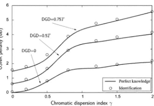
Fig. 2. OSNR penalty curves at BER= 10 .
In the operating conditions, the transmitted bits are not avail-able. Hence, we resort to a decision directed approach, that is we use the decisions of the VA entailing no performance loss at least when the bit-error rate (BER) is lower than . The de-cisions of the VA are available with a delay of symbols which can compromise the capability of the algorithm in tracking the fast channel variations. However, this is not the case of the con-sidered channel since the dispersion we are facing is a slowly varying phenomenon. For the same reason, it is not necessary to update the channel parameters at each bit interval but they can be updated less frequently, depending on the considered channel.
Considering now the initial acquisition of the algorithm, al-though a training sequence can be adopted to reduce the acqui-sition time, we verified by computer simulations that the algo-rithm is able to work in a completely blind manner, as discussed in Section IV.
IV. NUMERICALRESULTS
We consider an optical channel affected by first-order PMD (with a worst-case power splitting equal to 0.5), and GVD, quan-tified through the chromatic dispersion index
, where is the wavelength, is the bit rate, is the residual chromatic dispersion, and is the light speed [8]. Hence, the same value of corresponds to different residual dis-persions depending on the considered bit rate (e.g., given
the residual dispersion is equal to 392 ps/nm at Gb/s and to 24 ps/nm at Gb/s). The optical filter is mod-eled as a fourth-order Butterworth type with bandpass band-width equal to and the MLSD receiver is based on a VA working on, at most, a 128-state trellis [8]. In Fig. 2, we show the optical signal-to-noise ratio (OSNR) penalty, obtained by com-puter simulations, for increasing values of , and for different values of the PMD differential group delay. The solid lines refer to the ideal receiver and are obtained under the hypothesis of perfect knowledge of the channel parameters, whereas the cir-cles represent the performance of the receiver when using the discribed estimation algorithm. It can be seen that no loss in performance is entailed.
We now show that the algorithm is able to work in the deci-sion directed mode in a completely blind manner. We consider a particular case of bad channel impairment, where the chro-matic dispersion index is equal to one. At the beginning and for the first 10 000 bits, the algorithm is turnedOFF. In this case, for an OSNR (referred to a bandwidth equal to the bit rate) of 13 dB we have a BER of 0.25. Hence, we do not have reliable decisions. Nonetheless, when the estimation algorithm is turned
Fig. 3. MSE transient when the estimation algorithm is turned on.
ON, it is still able to converge to a BER of (the value cor-responding to perfect knowledge of the channel parameters) in about bits, as can be seen from Fig. 3 showing the time evolution of the MSE.
V. CONCLUSION
In the literature, the benefits of the application of MLSD to optical communication systems have been widely demon-strated. In this letter, we have shown that it is possible to adap-tively estimate the channel parameters, i.e., the noise-free sam-pled signal and the noise PSD, to be used in the computation of the branch metrics of the VA implementing the MLSD strategy. The performance of the proposed algorithm, in terms of con-vergence time and estimation accuracy, has been investigated. It has also been demonstrated that the performance of the pro-posed adaptive receiver is the same as that of the ideal receiver with perfect channel knowledge.
REFERENCES
[1] J. G. Proakis, Digital Communications, 3rd ed. New York: McGraw-Hill, 1996.
[2] J. H. Winters and R. D. Gitlin, “Electrical signal processing techniques in long-haul fiber-optic systems,” IEEE Trans. Commun., vol. 38, no. 9, pp. 1439–1453, Sep. 1990.
[3] J. H. Winters and S. Kasturia, “Adaptive nonlinear cancellation for high-speed fiber-optic systems,” J. Lightw. Technol., vol. 10, no. 7, pp. 971–977, Jul. 1992.
[4] H. Bulow and G. Thielecke, “Electronic PMD mitigation—From linear equalization to maximum-likelihood detection,” in Proc. OFC’01, 2001, vol. 3, pp. WDD34-1–WDD34-3.
[5] F. Buchali and H. Bulow, “Adaptive PMD compensation by elec-trical and optical techniques,” J. Lightw. Technol., vol. 22, no. 4, pp. 1116–1126, Apr. 2004.
[6] H. F. Haunstein, W. Sauer-Greff, A. Dittrich, K. Sticht, and R. Ur-bansky, “Principles for electronic equalization of polarization-mode dispersion,” J. Lightw. Technol., vol. 22, no. 4, pp. 1169–1182, Apr. 2004.
[7] O. E. Agazzi, M. R. Hueda, H. S. Carrer, and D. E. Crivelli, “Max-imum-likelihood sequence estimation in dispersive optical channels,”
J. Lightw. Technol., vol. 23, no. 2, pp. 749–763, Feb. 2005.
[8] T. Foggi, E. Forestieri, G. Colavolpe, and G. Prati, “Maximum like-lihood sequence detection with closed-form metrics in OOK optical systems impaired by GVD e PMD,” J. Lightw. Technol., vol. 24, no. 8, pp. 3073–3087, Aug. 2006.
[9] G. Bosco and P. Poggiolini, “Long-distance effectiveness of MLSE IMDD receivers,” IEEE Photon. Technol. Lett., vol. 18, no. 9, pp. 1037–1039, May 1, 2006.
[10] D. Marcuse, “Derivation of analytical expression for the bit-error probability in lightwave systems with optical amplifiers,” J. Lightw.
Technol., vol. 8, no. 12, pp. 1816–1823, Dec. 1990.
[11] P. A. Humblet and M. Azizog˜lu, “On the bit error rate of lightwave systems with optical amplifiers,” J. Lightw. Technol., vol. 9, no. 11, pp. 1576–1582, Nov. 1991.
[12] H. L. Van Trees, Detection, Estimation, and Modulation Theory—Part