Queueing models for air traffic

(1)

UNIVERSIT `A DEGLI STUDI DI ROMA “TOR VERGATA”

FACOLT `A DI SCIENZE MATEMATICHE, FISICHE E NATURALI

Dottorato in Matematica - Ph. D. in Mathematics XXI ciclo

Queueing models for air traffic

Coordinator:

Prof. Filippo Bracci

Supervisor: Candidate:

Prof. Benedetto Scoppola Dr. Sokol Ndreca

(2)

(3)

I dedicate this thesis to my mother Drande and to my father Simon.

(4)

(5)

Abstract

In this thesis we study some queueing models that are worthwhile to understand the air-traffic congestion. From the point of view of classical queueing theory the air air-traffic system is difficult to study, mainly because it is hard even to define the basic quantities of the theory. The system becomes complex, since there are a many factor, that influence the air-traffic like weather conditions, technical problems, air turbulences caused by the different types of aircrafts. Thus is necessary to investigate the impact of the arrivals of aircraft on air traffic. A common hypothesis in literature is to assume that the arrivals of aircrafts are very well modeled by a Poisson process. This assumption is suitable for mathematical modelling, due to the memoryless property of Poisson process that simplifies the study of congestion in such systems.

Our first goal is to study the property of a model of the arrival process to a system and to compare its features to the Poisson process. We will show in this work why the Poissonian hypothesis for air-traffic is doomed to failure even if the Poisson process is very similar to our process if it is observed on a time scale sufficiently short. We found interesting connections of this model with the statistical mechanics of Fermi particles.

Once one understands the properties of arrival process to the system, to study its evolution we use the theory of Markov chain.

Our second goal is the study of the stochastic properties of other queueing systems, relevant in the applications, where the arrivals are described according general independent stochastic process and the service is delivered according to various disciplines. This corresponds to the study of the stationary measure of a Markov chain. In order to find the stationary distribution of such Markov chain we use the generating function technique. Part of this thesis is a discussion of the criteria usually presented in literature to evaluate the goodness of various approximation schemes. It will turn out, actually, that the generating function is not always possible to compute explicitly, and some numerical procedures are necessary in order to compute the relevant quantities of the system.

Keywords: Queueing system, air-traffic congestion, non Poissonian arrivals, tail approx-imation, two class queue in parallel, priority and Bernoulli scheduling.

(6)

(7)

Riassunto

In questa tesi studiamo dei modelli di coda che sono utili per capire la congestione del traffico aereo. Dal punto di vista della teoria delle code classica e’ difficile studiare il sistema del traffico aereo, soprattutto perche’ e’ complesso definire le quantita’ di base della teoria. Il sistema diventa complesso, poiche’ ci sono molti fattori che influiscano sul traffico aereo, ad esempio le condizioni meteo, problemi tecnici, le turbolenze dell’aria causate da diversi tipi di aeromobili. Quindi per capire il traffico aereo diventa necessario studiare la distribuzione degli arrivi degli aeroplani. In letteratura l’ipotesi comune e’ di assumere che gli arrivi degli aeroplani sono descritti molto bene dal processo di Poisson. Questa assunzione e’ adatto per i modelli matematici, per la proprieta’ di assenza di memoria del processo di Poisson che semplifica lo studio della congestione in tale sistema.

Il primo obiettivo di questa tesi e’ di studiare le proprieta’ di un processo degli arrivi degli aeromobili al sistema e di confrontare tale processo con il processo di Poisson. In questo lavoro mostriamo come l’ipotesi Poissoniana per il traffico aereo e’ destinato a fallire anche se il processo Poissoniano e’ molto simile al nostro modello degli arrivi se viene osservato su una scala di tempo opportunamente corta.

Troviamo poi, nella trattazione del nostro processo, una connessione interessante del nostro modello con la meccanica statistica di Fermioni.

Una volta comprese le proprieta’ del processo degli arrivi al sistema, per studiare la sua evoluzione usiamo la teoria Markoviana.

Il secondo obiettivo di questa tesi e’ lo studio delle proprieta’ stocastiche di altri sistemi di coda, sempre rilevanti nelle applicazioni, in cui gli arrivi sono generali ma indipendenti, e discipline di servizio particolari rendono non banale lo studio della distribuzione stazionaria della catena. Questo corrisponde a studiare la misura stazionaria di certe catene di Markov. Per trovare la distribuzione stazionaria usiamo il metodo della funzione generatrice. Una parte di questa tesi e’ la discussione dei criteri, di solito presentati in letteratura, per valutare l’ottimalita’ dei vari schemi di approssimazione.

Parole chiave: Sistema di coda, traffico aereo congestionato, arrivi non Poissoniani, approssimazione coda, due classi di coda in parallelo, priorita’ e scheduling Bernoulliano.

(8)

(9)

Introduction and Motivation

To wait, or not to wait: that is the queue!

In this thesis we study some queueing models that are worthwhile to understand the air-traffic congestion. From the point of view of classical queueing theory the air traffic system is difficult to study, mainly because it is hard even to define the basic quantities of the theory. The system becomes complex, since there are a many factor, that influence the air-traffic like weather conditions, technical problems, air turbulences caused by the different types of aircrafts. For instance it is clear that there is some congestion for landing aircrafts, since they have to follow some holding paths, but it is not easy to quantify the actual time spent in queue or even its instant length. On the other hand, even assuming that the parameters of the system are known, it is not clear what kind of point processes are suitable to describe arrivals and service times. Thus is obviously necessary, to investigate the impact of the arrivals of aircrafts on air traffic. A common hypothesis in literature is to assume that the arrivals of aircrafts are very well modeled by a Poisson process. This assumption is very suitable for mathematical modelling, due to the memoryless property of Poisson process that simplifies the study of congestion in such system.

Our first goal is to study the property of arrival process to a system. We will show in this work why the Poissonian hypothesis for air-traffic is doomed to failure.

Once one understands the properties of arrival process to a system, to study the evolution of system we use the theory of Markov chain.

Our second goal is the study of the stochastic properties of other queueing system, where the arrivals are described according general independent stochastic process and the service is delivered according to various disciplines. This corresponds to the study of stationary measure of Markov chains. In order to find the stationary distribution of Markov chain we use the generating function technique. Part of this thesis is a discussion of the criteria usually presented in literature to evaluate the goodness of various approximation schemes. It will turn out, actually, that the generating function is not always possible to compute explicitly, and some numerical procedures are necessary in order to compute the relevant quantities of the system.

(12)

1.1 Stochastic point process as arrival process

Poissonian hypothesis for air traffic arrivals, to our knowledge, goes back to the 70’s when Dunlay and Horonjeff gave in [17] a number of theoretical and statistical arguments to justify this assumption, and, since then, several other statistical studies have supported the same results. Even recently, see [16], a very careful study of the interarrival times of aircrafts to major US airports shows a small difference between the Poisson and the observed distribution, i.e. the actual arrivals are slightly less random than Poissonian ones, but the difference is quite small in all observed airports. On this ground, in various papers, see for instance [18], [21] and [22] and reference therein, Poisson arrivals have been assumed in the analysis of judicious management of service times. It should be stressed that in all these papers the statistical validation of the Poissonian hypothesis has been based on computations on time scales smaller than the intrinsic randomness of the system. The fact that arrivals are prescheduled clearly make the Poissonian hypothesis questionable. If we forecast a reduction of the intrinsic variability of arrival times, which could be achieved by various technical improvements (e.g. a rescheduling closer to the actual arrival times, or an en-route control of the paths of the aircrafts), we should expect the Poissonian assumption to fail, because it depends only on a single parameter 𝜌. About the stochastic models of aircraft arrivals we consider a point process defined as follows

𝑡𝑖 = 𝑖

𝜆+ 𝜉𝑖 (1.1)

where 𝑖 ∈ Z, the 𝜉𝑖 are i.i.d. random variables with variance 𝜎2 eventually much larger than 1

𝜆 and 1

𝜆 is the expected interarrival time between two aircrafts. From now on, we will call this process pre-scheduled random arrivals (PSRA) process. Note that this arrival process, excepted the presence of cancellations and pop-ups1_{, is exactly the actual arrival process} introduced in [4] using for 𝜉𝑖 a uniform distribution. This process that we will study in chapter 2 is an arrivals model with two features. First, it shows a pattern of arrivals very close to a Poisson process when we look at time scales smaller than the standard deviation of aircraft delays, second, it provides the distribution of arrivals on time scales larger or comparable to the standard deviation of aircraft delays.

We study more rigorously the features of arrival process presented in [4], which we suitably generalize, and to understand its analytical properties, we show that this process, with a suitable rescaling of the distribution of 𝜉𝑖’s, converges to the Poisson process in total variation for large 𝜎, so

∞ ∑︁

𝑛=0

|𝑞(𝜎)_𝑛 − 𝑞𝑛| → 0 as 𝜎 → ∞ (1.2)

where the sequence 𝑞𝑛(𝜎)and 𝑞𝑛are the coefficient of generating function of PSRA process and Poisson process respectively. Moreover, we show, both analytically and numerically, that the congestion related to this process is very different from the congestion of a Poisson process, on any time scale. This is due to the negative autocorrelation of the process, as we prove explicitly.

1_{Pop-ups are flights that arrive at the airport but were not expected on the time the GDP was}

imple-mented. A Ground Delay Program (GDP) is a traffic flow initiative that is instituted by the Federal Aviation Administrative (FAA) in the US.

(13)

1.2. MODEL WITH VARIABLE NUMBER OF SERVERS 3

1.2 Model with variable number of servers

The multi-server queueing system, with Poisson arrivals and deterministic service time, de-noted usually by 𝑀/𝐷/𝑐 has a long history. The system was initially ideated by Erlang (see e.g. [11]) and later studied in [9, 10, 19], using theory of complex analysis. They describe the generating function of the system in terms of the root of the denominator inside the unit disc. Nevertheless, the problem to find the 𝑐 complex root inside the unit disc is still studied. In this context, we will consider the systems with general arrivals, a variable number of servers, that is a system in which 𝑐 is a random variable. This is because we want to study simple models of a discrete time services in which the number of servers at each time is the independent realization of a given random variable with distribution 𝛼𝑙= 𝑃 (𝑐𝑖= 𝑙) i.e. 𝛼𝑙 is the probability that the users2 find 𝑙 available severs. A very natural example: in an airport, due to the safety rules for air traffic, some runways may be momentarily unavailable when some other runways are used by aircrafts in certain conditions. Hence the number of runways available in each time slot3 may vary very rapidly.

We write the exact generating function in terms of 𝑐 singularities 𝑧1, ...𝑧𝑐 of denominator in the unit disc, which represent the exact solution of problem, that gives us the knowledge of the queueing system. Nevertheless, the solution has two main disadvantages. First, it is not always easy to find complex zeroes of denominator, especially when 𝑐 is large. Second, a small error (always present in numerical computations) on the values of 𝑧1, ...𝑧𝑐 generates a sequence of 𝑃𝑛 that rapidly diverges from the true (probabilistic) expression. We show that if 𝑧1, ...𝑧𝑐 do not cancel exactly the zeroes of the denominator in the generating function, the latter diverges in some 𝑧𝑖 and their coefficients 𝑃𝑛 diverge exponentially, loosing their probabilistic interpretation. We therefore define a suitable approximation schemes for infinite Markov chain in order to avoid the explicit computation of such singularities.

The basic idea of this approximation scheme is as follows: we describe the system starting from the cumulative probabilities 𝜎𝑛:=∑︀𝑛𝑘=0𝑃𝑛and in order to have a probabilistic interpre-tation, the sequence of 𝜎𝑛 has to be increasing, 𝜎𝑖 ≤ 𝜎𝑖+1 and lim𝑛→∞𝜎𝑛= 1. Let {^𝜎𝑛}𝑛≥0 and {𝜎}𝑛≥0 be the solution of the infinite system and truncated system respectively and also let us define by Δ𝑛:= 𝜎𝑛− ^𝜎𝑛the errors of approximation; thus due to the linearity of system representing the 𝜎𝑛’s, we can write it in terms of Δ𝑛’s. We will study the property of errors Δ𝑛’s of approximation. We will present a rephrasing of one of the most used approximation schemes, the so-called last column augmentation, and we will discuss some theoretical and numerical results about the errors involved in this approximation.

We will show that an optimal approximation scheme, the censored Markov chain, gives often a bigger error than augmentation procedure in the part of the distribution that is relevant in the computation of the average values. Also with our approximation scheme we give an estimate on the errors in the sense of the 𝐿∞ norm, then

2_{In this thesis we use the term “user” in a general sense.} 3

In this thesis we assume that the time is divided into fixed length intervals or slots. The users arrive in the system according to a general arrival process during the consideration and the consecutive slot, but they can receive service only at pre-defined discrete times, so at the beginning of slot

(14)

1.3 Two queues in parallel

Let us now consider a simplified description of the following problem: the air traffic is com-posed of different types of aircrafts, implying different queueing costs as well or different service times. Hence a non realistic description has to take into account the existence of different classes of users. Let us now consider the system, when two classes of users arrive to a single server, according to a general independent stochastic process. We can think this system composed of two separate queues in parallel, where the each one of users belonging to each queue are served according to FIFO discipline. We discus two cases: 1) users of first class have a higher priority than users of second class, or in other words the users of second class can be served only if the users of first class are absent. 2) users of first class receive service with probability 𝑝 (0 ≤ 𝑝 ≤ 1) and the users of second class receive service with probability 1 − 𝑝 (Bernoulli scheduling) if the two classes are both non empty. To understand these typology of system we describe it as a Markov chain with two dimensional probabil-ity generating function. In this way we obtain a generating function which contain some unknown functions. In order to find the unknown functions we use the theory of boundary value problem. So, the problem to finding the stationary joint probability distribution can be reduced to solve the boundary value problem.

Fayolle and Iasnogorodski in [12] studied two queueing in parallel, with Poisson arrivals and exponential service times and single server; using the Riemann Hilbert boundary value problem they found the joint generating function. Later Cohen and Boxma in [15] described in general the boundary value problem in queueing theory.

In the first case i.e. a simple priority rule, that will we study in chapter 4, the generating function contains a single unknown function. We study the condition for the existence of solution of boundary value problem and we solve it. In this way we control completely the generating function.

The study of second case is more difficult, because the generating function contain two unknown functions. The idea to bypass this difficulty is to use the perturbative method. Clearly the generating function depends on 𝑝 and for 𝑝 = 1 and 𝑝 = 0 the generating function has the same structure as the generating functions of system discussed in the first case, hence we have the exact solution of problem for 𝑝 = 1 and 𝑝 = 0 as we will prove in chapter 4. Now expanding the generating function in powers of 1 − 𝑝 and 𝑝 on appropriate domain we obtain two sequence of functional coefficients that are symmetric in 𝑥 and 𝑦. Using these coefficients and exact solution of problem for 𝑝 = 1 and 𝑝 = 0 we will give the approximate solution of generating function. In order to prove the validity of approximation method we present some numerical results for lower and heavy traffic intensity and varying of parameter 𝑝.

1.4 The map of thesis

The thesis is organized as follows:

In chapter 2, we propose the PSRA process as arrival process, that is alternative of Poisson process to describe the arrivals of aircrafts. We study the property of this stochastic point process through the use of generating function and compare its feature to Poisson process. In chapter 3, we investigate the model with fixed and variable number of servers. We give a suitable approximation scheme for infinite Markov chain in order to obtain the average of the queue length.

(15)

1.4. THE MAP OF THESIS 5

where the users of first class have a higher priority than users of second class. We obtain the generating function of the joint stationary probability distribution through the solution of the boundary problem. Moreover we study the discrete time single server queueing with Bernoulli scheduling and two classes of users. We give the approximation solution of generating function through perturbative method.

(16)

(17)

Chapter 2

Queueing system with

pre-scheduled random arrivals

In this chapter we consider a point process obtained summing a random variable 𝜉𝑖 to each point 𝑖 of the set of integer Z. The 𝜉𝑖’s are i.i.d. random variables with variance 𝜎2 eventually much larger than 1. We compare the process obtained with this construction with the Poisson process. Moreover, we show that, this process, with a suitable rescaling of the distribution of 𝜉𝑖’s, converges to the Poisson process in total variation for large 𝜎. We then study a simple queueing system with our process as arrival process, and we provide some analytical and numerical results.

2.1 Introduction

The main aim of this chapter is to define a stochastic point process and to compare its features to the Poisson process. It is well known that the memoryless property of the Poisson process simplifies many technical steps in the analysis of queueing systems, but there are arrival processes where such an assumption is not completely satisfied. In particular, we have in mind air traffic models.

Stochastic models of aircraft arrivals based on statistical analysis and on simulations have a long history. As a first attempt, Barnett et al. [1] studied the arrivals to Boston Logan Airport. A version of the alternative model of arrivals we propose in this chapter was introduced and studied numerically in [4]. The model is refined in [3], where seasonal and daily effects are taken into account to describe random delays of departure times and, with these corrections, the model is quite accurate in its predictions. The key feature of the model is a soft a-prior scheduling of arrivals: indeed, both in US and in Europe, aircrafts are supposed to take off and to land by a schedule dictated by the capacity constraint of the runways, and by the assumption that each aircraft would land in a very narrow time slot. However, on the day of operations, an aircraft will be declared ”on time” if it lands in a time interval larger than ten times the original slot. In this sense the scheduling should be considered ”soft”.

The process we study below is an arrivals model with two features. First, it shows a pattern of arrivals very close to a Poisson process when we look at time scales smaller than the standard deviation of aircraft delays, second, it provides the distribution of arrivals on

(18)

time scales larger or comparable to the standard deviation of aircraft delays.

Thus, the aim of this chapter is an attempt to study more rigorously the features of arrival process presented in [4], which we suitably generalize, and to understand its analytical properties.

Moreover, we compare, both analytically and numerically, the queueing system in which the arrivals are described according to a Poisson process and a PSRA process respectively and for the second system we give the expression for the stationary probability distribution, under the hypothesis that the number of arrivals in subsequent slot are independent random variable. We can consider that stationary distribution like lower bound for the stationary distribution for the 𝑀/𝐷/1 queueing system.

The analytical description of the system clarifies many interesting features of this kind of traffic: for heavy traffic the system has a long memory of the initial conditions; its description is obtained by the superposition of two processes, living on different time scales. This give the possibility to investigate also systems with slowly variable traffic intensities.

The chapter is organized as follows: in section 2.2 we describe our arrival process, and we list some results on the comparison to the Poisson process. In section 2.3 we present a simplified computation, which shows that congestion levels according to our process are quite different from the Poisson process. However, in section 2.4 we show numerically that our approximation is bad for very congested systems, and the actual level of congestion is even more different than the Poissonian one. In section 2.5 we describe completely our queueing system at the price to enlarge suitably the state space of the Markov chain describing it. It turns out that for our process we have a finite value of the expected queue length even in the critical case 𝜚 = 1, while the Poisson queue diverges. Starting from the results on the critical case, we propose an approximation scheme that works very well for highly congested (𝜚 near to 1) systems. In this description a nice connection with the statistical mechanics of Fermi gas emerges quite naturally. Section 2.6 is devoted to conclusions and open problems.

2.2 Description of the model: the arrival process

The queueing model we study is defined by a single server with deterministic service time and an arrival process, which we will call pre-scheduled random arrivals (PSRA) process, defined as follows. Let 1_𝜆 be the expected interarrival time between two users, we define 𝑡𝑖 ∈ R the actual arrival time of the 𝑖-th user by

𝑡𝑖 = 𝑖

𝜆+ 𝜉𝑖 𝑖 ∈ Z (2.1)

where 𝜉𝑖’s are i.i.d. random variables.

If the 𝜉𝑖’s are uniform, the model is the actual arrival times process introduced in [4] without cancellations and pop-ups, which could be easily integrated into the process. From now on, we will assume that 𝜉𝑖’s have continuous probability density 𝑓_𝜉(𝜎)(𝑡) with variance 𝜎2, and we will set without loss of generality 𝐸(𝜉𝑖) = 0, since 𝐸(𝜉𝑖) ̸= 0 affects only the initial configuration of the system. The main aim of this section is to compare the features of the PSRA process to the Poisson process when 𝜎 is large. It is well known, e.g. [2, p.447], that the Poisson arrival process is defined by the fact that probabilities 𝑃𝑗,𝑗+1(Δ𝑡) = 𝑃 (𝑛(𝑡 + Δ𝑡) = 𝑗 + 1|𝑛(𝑡) = 𝑗) of a ”jump” from the state 𝑗 to the state 𝑗 + 1 in the time interval (𝑡, 𝑡 + Δ𝑡] have the form

(19)

2.2. DESCRIPTION OF THE MODEL: THE ARRIVAL PROCESS 9

where 𝜆 is a constant independent of 𝑡 and 𝑗; 𝜆 has the meaning of velocity of arrivals, i.e. denoting with 𝑡𝑎 the interarrival time, 𝐸(𝑡𝑎) = 1_𝜆. For pre-scheduled random arrivals the probability 𝑃 (𝑖, 𝑡, Δ𝑡) that the 𝑖-th user arrives in the time interval (𝑡, 𝑡 + Δ𝑡] is given by

𝑃 (𝑖, 𝑡, Δ𝑡) = 𝑃 (︂ 𝑡 < 𝑖 𝜆+ 𝜉𝑖< 𝑡 + Δ𝑡 )︂ = (2.3) = 𝑃 (︂ 𝑡 − 𝑖 𝜆< 𝜉𝑖< 𝑡 + Δ𝑡 − 𝑖 𝜆 )︂ = ∫︁ 𝑡+Δ𝑡−𝑖 𝜆 𝑡−_𝜆𝑖 𝑓_𝜉(𝜎)(𝑥)𝑑𝑥 (2.4) and, for small Δ𝑡, it may be written as

𝑃 (𝑖, 𝑡, Δ𝑡) = 𝑓_𝜉(𝜎) (︂ 𝑡 − 𝑖 𝜆 )︂ Δ𝑡 + 𝑜(Δ𝑡) (2.5)

By (2.5), the probability 𝑃+(𝑡, Δ𝑡) of a single PSRA arrival in the interval (𝑡, 𝑡 + Δ𝑡] is 𝑃+(𝑡, Δ𝑡) =∑︁ 𝑖∈Z 𝑃 (𝑖, 𝑡, Δ𝑡)∏︁ 𝑗̸=𝑖 (1 − 𝑃 (𝑗, 𝑡, Δ𝑡)) = =∑︁ 𝑖∈Z [︂ 𝑓_𝜉(𝜎) (︂ 𝑡 − 𝑖 𝜆 )︂ Δ𝑡 + 𝑜(Δ𝑡) ]︂ exp ⎛ ⎝ ∑︁ 𝑗̸=𝑖 log [︂ 1 − 𝑓_𝜉(𝜎) (︂ 𝑡 − 𝑗 𝜆 )︂ Δ𝑡 + 𝑜(Δ𝑡) ]︂ ⎞ ⎠ (2.6) and 𝑃+(𝑡, Δ𝑡) =∑︁ 𝑖∈Z [︂ 𝑓_𝜉(𝜎) (︂ 𝑡 − 𝑖 𝜆 )︂ Δ𝑡 + 𝑜(Δ𝑡) ]︂ exp ⎛ ⎝−∑︁ 𝑗̸=𝑖 [︂ 𝑓_𝜉(𝜎) (︂ 𝑡 − 𝑗 𝜆 )︂ Δ𝑡 + 𝑜(Δ𝑡) ]︂ ⎞ ⎠ (2.7)

Hence up to the first order in Δ𝑡 the rate of arrival 𝜆(𝑡) of the pre-scheduled random arrivals is defined by 𝜆(𝑡) =∑︁ 𝑖∈Z 𝑓_𝜉(𝜎) (︂ 𝑡 − 𝑖 𝜆 )︂ (2.8) This rate 𝜆(𝑡) is periodic in 𝑡 with period _𝜆1, but it has an explicit dependence on 𝑡. However we are interested in the dependence of 𝜆(𝑡) on 𝜎, in particular when 𝜎 is large with respect to _𝜆1. To prove limit properties for our process, we have to specify the way we want to send 𝜎 to infinity. We will require the following scaling property for the density 𝑓_𝜉(𝜎)(𝑡).

Assumptions 2.2.1. The probability density of 𝜉 has the form 𝑓_𝜉(𝜎)(𝑡, 𝜎2) = 1

𝜎𝑓𝜉(𝑡/𝜎) (2.9)

i.e. it is the rescaling of a well defined continuous density 𝑓𝜉(𝑡) with finite variance. We will also write max_𝑡∈R𝑓𝜉(𝑡) = 𝑀 .

This assumption is introduced in order to exclude pathological ways to send 𝜎 to infinity, as, for instance, to have a bimodal distribution with fixed maxima, see figure 2.1.

For example Gaussian, Exponential, Gamma, and Uniform random variables satisfy this property. It follows that, in the limit 𝜎 very large the expression

𝑅(𝜎, 1/𝜆) :=∑︁ 𝑖∈Z 1 𝜆𝑓 (𝜎) 𝜉 (︂ 𝑡 − 𝑖 𝜆 )︂ (2.10)

(20)

Figure 2.1: A bimodal distribution with fixed shapes shifting to infinity for 𝜎 → ∞.

is the Riemann integral of the function 𝑓_𝜉(𝜎)(𝑡). For example, let 𝜉 be Gaussian 𝑁 (0, 𝜎2),

𝑅(𝜎, 1/𝜆) =∑︁ 𝑖∈Z 1 𝜆 1 √ 2𝜋𝜎2𝑒 −(𝜆𝑡−𝑖)2 2𝜎2𝜆2 = ∑︁ 𝑖∈Z 1 √ 2𝜋𝑒 −1 2( 𝑡𝜆−𝑖 𝜆𝜎 ) 2 ₁ 𝜆𝜎 = ∑︁ 𝑖∈Z 1 √ 2𝜋𝑒 −𝑥2𝑖 2 Δ𝑥 −→ 1

where 𝑥𝑖 = 𝜆𝑡−𝑖_𝜆𝜎 and Δ𝑥 = _𝜆𝜎1 and the limit is for 𝜎 → ∞.

For any random variable rescaled in the above sense it is clear that the result lim

𝜎2_→∞𝑅(𝜎, 1/𝜆) = 1 (2.11)

holds, and therefore, in the same limit, lim

𝜎2_→∞𝜆(𝑡) = lim𝜎→∞𝜆𝑅(𝜎, 1/𝜆) = 𝜆 (2.12)

It is interesting, for Gaussian 𝜉, to check numerically how fast the limit is reached. Table 2.1 shows it. For simplicity, we set 𝜆 = 1.

0 0.1 0.2 0.3 0.4 0.5 0.6 0.7 0.8 0.9 1 t 0 0.2 0.4 0.6 0.8 1 1.2 1.4 1.6 1.8 2 λ(σ, t) λ(σ,0) λ(.8,t) λ(.2,t)

Figure 2.2: Behavior of the function 𝜆(𝜎, 𝑡)

The graph in figure 2.2 shows that, in terms of rate of arrivals, the pre-scheduled random arrivals approach the Poisson process when 𝜎 is suitably large. In particular for Gaussian variables with standard deviation 𝜎 of order 1/𝜆 we have that 𝜆(𝑡) tends to be constant. Note

(21)

2.2. DESCRIPTION OF THE MODEL: THE ARRIVAL PROCESS 11 𝜎 𝜆(0) 𝜆(0.1) 𝜆(0.2) 𝜆(0.3) 𝜆(0.4) 𝜆(0.5) .2 1.994726 1.760407 1.210523 0.651951 0.292114 0.175283 .3 1.340089 1.274318 1.103259 0.894087 0.726696 0.663191 .4 1.085005 1.068767 1.026261 0.973729 0.931237 0.915008 .5 1.014384 1.011637 1.004445 0.995555 0.988363 0.985616 .6 1.00164 1.001327 1.000507 0.999493 0.998673 0.99836 .7 1.000126 1.000102 1.000039 0.999961 0.999898 0.999874 .8 1.000007 1.000005 1.000002 0.999998 0.999995 0.999993 .9 1. 1. 1. 1. 1. 1. 1. 1. 1. 1. 1. 1. 1. 𝜎 𝜆(0.6) 𝜆(0.7) 𝜆(0.8) 𝜆(0.9) 𝜆(1) .2 0.292114 0.651951 1.210523 1.760407 1.994726 .3 0.726696 0.894087 1.103259 1.274318 1.340089 .4 0.931237 0.973729 1.026261 1.068767 1.085005 .5 0.988363 0.995555 1.004445 1.011637 1.014384 .6 0.998673 0.999493 1.000507 1.001327 1.00164 .7 0.999898 0.999961 1.000039 1.000102 1.000126 .8 0.999995 0.999998 1.000002 1.000005 1.000007 .9 1. 1. 1. 1. 1. 1. 1. 1. 1. 1. 1. Table 2.1:

that for applications mentioned in the introduction, we do expect the standard deviation to be much larger than 1/𝜆. Note also that the explicit structure of the density of 𝜉 does not play any particular role, and similar results may be obtained with different distributions. However it is clear that a small dependence on 𝑡 is always present in the expression of 𝜆(𝑡), and hence it is difficult to obtain a quantitative comparison between the pre-scheduled random arrivals and the Poisson process on this basis, therefore we look at the distribution of the random variable 𝑛(𝑡, 𝑡 + 𝑇 ), number of arrivals in the finite interval (𝑡, 𝑡 + 𝑇 ]. So the random variable 𝑛(𝑡, 𝑡 + 𝑇 ) count the number of arrivals in the interval (𝑡, 𝑡 + 𝑇 ]. Let us call 𝑝𝑖(𝑡, 𝑡 + 𝑇 ) the probability that the 𝑖-th user arrives in the interval (𝑡, 𝑡 + 𝑇 ]. Clearly

𝑝𝑖(𝑡, 𝑡 + 𝑇 ) = ∫︁ 𝑡+𝑇 𝑡 𝑓_𝜉(𝜎) (︂ 𝑥 − 𝑖 𝜆 )︂ 𝑑𝑥 (2.13)

Given the probabilities 𝑝𝑖(𝑡, 𝑡+𝑇 ) we can write the generating function of the random variable 𝑛(𝑡, 𝑡 + 𝑇 ), and, defining 𝑞𝑛(𝜎)= 𝑃 (𝑛(𝑡, 𝑡 + 𝑇 ) = 𝑛) we get

𝑞(𝜎)_𝑛 = ∑︁ 𝐼={𝑖1,...,𝑖𝑛} ∏︁ 𝑖∈𝐼 𝑝𝑖(𝑡, 𝑡 + 𝑇 ) ∏︁ 𝑗 /∈𝐼 (1 − 𝑝𝑗(𝑡, 𝑡 + 𝑇 )) (2.14)

where the sum runs over all the possible distinct subsets 𝐼 of indices of cardinality 𝑛. By mean of this expression one obtains the generating function

𝑞(𝜎)(𝑧) =∑︁ 𝑛≥0

𝑞(𝜎)_𝑛 𝑧𝑛=∏︁ 𝑖∈Z

(1 + (𝑧 − 1)𝑝𝑖(𝑡, 𝑡 + 𝑇 )) (2.15)

To take into account also the possibility of random independent deletion as in [4], let us outline here that a similar generating function can be introduced also when each arrival has

(22)

an independent probability 1 − 𝛾 to be deleted, and the complementary probability 𝛾 to be an actual arrival. In other words, we construct the PSRA process for 𝑖 ∈ Z and then for each 𝑖 we cancel the corresponding 𝑖-th arrival with independent probability 1 − 𝛾. It is obvious that in this case the generating function is

𝑞_𝛾(𝜎)(𝑧) =∑︁ 𝑛≥0

𝑞_𝛾,𝑛(𝜎)𝑧𝑛=∏︁ 𝑖∈Z

(1 + (𝑧 − 1)𝛾𝑝𝑖(𝑡, 𝑡 + 𝑇 )) (2.16)

The expression (2.15) are exact, and gives us all the information on the distribution of 𝑛(𝑡, 𝑡 + 𝑇 ), and it depends explicitly on 𝑡 and 𝑇 . However we can study 𝑞(𝜎)(𝑧) and 𝑞(𝜎)𝛾 (𝑧) for large 𝜎, in the sense of the rescaling defined above, and show that they converges to a Poisson distribution with parameter 𝜆𝑇 and 𝛾𝜆𝑇 . The main idea is to exploit the fact that, for large 𝜎, 𝑝𝑖(𝑡, 𝑡 + 𝑇 ) goes to zero as 1_𝜎.

We now prove the following results. Lemma 2.2.2. max 𝑖 𝑝𝑖(𝑡, 𝑡 + 𝑇 ) ≤ 𝑐𝑜𝑛𝑠𝑡(𝑇 ) 𝜎 (2.17) Proof. 𝑝𝑖(𝑡, 𝑡 + 𝑇 ) = ∫︁ 𝑡+𝑇 𝑡 𝑓_𝜉(𝜎) (︂ 𝑥 − 𝑖 𝜆 )︂ 𝑑𝑥 = ∫︁ 𝑡−_𝜆𝑖+𝑇 𝑡−_𝜆𝑖 𝑓_𝜉(𝜎)(𝑠)𝑑𝑠 = 1 𝜎 ∫︁ 𝑡−_𝜆𝑖+𝑇 𝑡−_𝜆𝑖 𝑓𝜉 (︁𝑠 𝜎 )︁ 𝑑𝑠 (2.18)

by the Intermediate Value Theorem 𝑝𝑖(𝑡, 𝑡 + 𝑇 ) = 1 𝜎𝑓𝜉 (︂ 𝑠* 𝑖 𝜎 )︂ 𝑇 ≤ 𝑀 𝑇 𝜎 (2.19) where 𝑠*_𝑖 𝜎 ∈ (︂ 𝑡 − 𝑖 𝜆, 𝑡 − 𝑖 𝜆+ 𝑇 )︂

Now we will use lemma 2.2.2 to bound the generating function

𝑞(𝜎)(𝑧) = exp [︃ ∑︁ 𝑖∈Z ln(1 + (𝑧 − 1)𝑝𝑖(𝑡, 𝑡 + 𝑇 )) ]︃ = (2.20) = exp [︃ (𝑧 − 1)∑︁ 𝑖∈Z 𝑝𝑖(𝑡, 𝑡 + 𝑇 ) (︂ 1 + (𝑧 − 1)𝑝𝑖(𝑡, 𝑡 + 𝑇 ) ∫︁ 1 0 𝑠 𝑑𝑠 (1 + (𝑧 − 1)(1 − 𝑠)𝑝𝑖(𝑡, 𝑡 + 𝑇 ))2 )︂]︃ (2.21) Lemma 2.2.3. With 𝑝𝑖(𝑡, 𝑡 + 𝑇 ) defined as above, the sum in (2.21) converges to 𝜆𝑇

lim 𝜎→∞ ∑︁ 𝑖∈Z 𝑝𝑖(𝑡, 𝑡 + 𝑇 ) (︂ 1 + (𝑧 − 1)𝑝𝑖(𝑡, 𝑡 + 𝑇 ) ∫︁ 1 0 𝑠 𝑑𝑠 (1 + (𝑧 − 1)(1 − 𝑠)𝑝𝑖(𝑡, 𝑡 + 𝑇 ))2 )︂ = 𝜆𝑇 (2.22)

(23)

2.2. DESCRIPTION OF THE MODEL: THE ARRIVAL PROCESS 13

Proof. First we prove that

lim 𝜎→∞

∑︁

𝑖∈Z

𝑝𝑖(𝑡, 𝑡 + 𝑇 ) = 𝜆𝑇. (2.23)

Let us define 𝑇 := 𝐾+Δ𝑇_𝜆 , where 𝐾 ∈ Z+ and 0 ≤ Δ𝑇 < 1. Then we can write

∑︁ 𝑖∈Z 𝑝𝑖(𝑡, 𝑡 + 𝑇 ) = ∑︁ 𝑖∈Z ∫︁ 𝑡−_𝜆𝑖+𝑇 𝑡−_𝜆𝑖 𝑓_𝜉(𝜎)(𝑠)𝑑𝑠 =∑︁ 𝑖∈Z ∫︁ 𝑡+𝐾−𝑖_𝜆 +Δ𝑇_𝜆 𝑡−_𝜆𝑖 𝑓_𝜉(𝜎)(𝑠)𝑑𝑠 = =∑︁ 𝑖∈Z ∫︁ 𝑡+𝐾−𝑖 𝜆 𝑡−𝑖 𝜆 𝑓_𝜉(𝜎)(𝑠)𝑑𝑠 +∑︁ 𝑖∈Z ∫︁ 𝑡+𝐾−𝑖 𝜆 + Δ𝑇 𝜆 𝑡+𝐾−𝑖_𝜆 𝑓_𝜉(𝜎)(𝑠)𝑑𝑠 (2.24)

The first term on the right hand side of (2.24) is 𝐾. Let 𝑖 = 𝑚𝐾 + 𝑙, where 𝑙 ∈ Z+ and 𝑚 ∈ Z, ∑︁ 𝑖∈Z ∫︁ 𝑡+𝐾−𝑖 𝜆 𝑡−_𝜆𝑖 𝑓_𝜉(𝜎)(𝑠)𝑑𝑠 = 𝐾−1 ∑︁ 𝑙=0 ∑︁ 𝑚∈Z ∫︁ 𝑡−(𝑚−1)𝐾+𝑙 𝜆 𝑡−𝑚𝐾+𝑙_𝜆 𝑓_𝜉(𝜎)(𝑠)𝑑𝑠 = 𝐾−1 ∑︁ 𝑙=0 ∫︁ R 𝑓_𝜉(𝜎)(𝑠)𝑑𝑠 = 𝐾 (2.25)

The second term on the right hand side of (2.24) converges to Δ𝑇 for 𝜎 → ∞: ∑︁ 𝑖∈Z ∫︁ 𝑡+𝐾−𝑖 𝜆 + Δ𝑇 𝜆 𝑡+𝐾−𝑖_𝜆 𝑓_𝜉(𝜎)(𝑠)𝑑𝑠 =∑︁ 𝑖∈Z ∫︁ 𝑡+𝑖 𝜆+ Δ𝑇 𝜆 𝑡+𝑖 𝜆 𝑓_𝜉(𝜎)(𝑠)𝑑𝑠 =∑︁ 𝑖∈Z 1 𝜎 ∫︁ 𝑡+𝑖 𝜆+ Δ𝑇 𝜆 𝑡+𝑖 𝜆 𝑓𝜉 (︁𝑠 𝜎 )︁ 𝑑𝑠 (2.26)

and, by the Intermediate Value Theorem we get ∑︁ 𝑖∈Z 1 𝜎 ∫︁ 𝑡+𝐾−𝑖 𝜆 + Δ𝑇 𝜆 𝑡+𝐾−𝑖_𝜆 𝑓𝜉 (︁𝑠 𝜎 )︁ 𝑑𝑠 =∑︁ 𝑖∈Z 1 𝜎𝑓𝜉 (︂ 𝑠* 𝑖 𝜎 )︂ Δ𝑇 𝜆 (2.27) where 𝑠*_𝑖 𝜎 ∈ (︂ 𝑡 + 𝐾 − 𝑖 𝜆 , 𝑡 + 𝐾 − 𝑖 𝜆 + Δ𝑇 𝜆 )︂ and finally, Δ𝑇 ∑︁ 𝑖∈Z 𝑓𝜉 (︂ 𝑠*_𝑖 𝜎 )︂ 1 𝜆𝜎 −→ Δ𝑇 (2.28)

as 𝜎 → ∞, where the sum on the last equality is the Riemann sum of 𝑓𝜉(𝑡). This ends the proof of (2.23). In order to complete the lemma we need to show that, uniformly in 𝑖,

lim 𝜎→∞(𝑧 − 1)𝑝𝑖(𝑡, 𝑡 + 𝑇 ) ∫︁ 1 0 𝑑𝑠 𝑠 (1 + (𝑧 − 1)(1 − 𝑠)𝑝𝑖(𝑡, 𝑡 + 𝑇 ))2 = 0 but this follows from lemma 2.2.2 and from the fact that

(𝑧 − 1) ∫︁ 1 0 𝑑𝑠 𝑠 (1 + (𝑧 − 1)(1 − 𝑠)𝑝𝑖(𝑡, 𝑡 + 𝑇 ))2 ≤ 𝐶 for any 𝑝𝑖(𝑡, 𝑡 + 𝑇 ) < 1/2 and |𝑧| ≤ 1.

(24)

Lemma 2.2.4. Let 𝑞(𝑧) = exp(𝜆𝑇 (𝑧 − 1)) be the probability generating function of the Pois-son random variable 𝜁 with intensity 𝜆𝑇 , and 𝑞𝛾(𝑧) = exp(𝛾𝜆𝑇 (𝑧 − 1)) be the probability generating function of the Poisson random variable 𝜁 with intensity 𝛾𝜆𝑇 , then

lim 𝜎→∞𝑞 (𝜎)_{(𝑧) = 𝑞(𝑧);} _lim 𝜎→∞𝑞 (𝜎) 𝛾 (𝑧) = 𝑞𝛾(𝑧) (2.29)

Proof. Follows immediately from lemma 2.2.3. Theorem 2.2.5. If 𝑞(𝜎)(𝑧) −→ 𝑞(𝑧), then ∑︀∞

𝑛=0|𝑞 (𝜎)

𝑛 − 𝑞𝑛| −→ 0 as 𝜎 → ∞. The same result holds for the arrivals with random deletions.

Proof. The proof follows from the continuity theorem for probability generating function see Feller [2, p.280].

Hence the PSRA process converges in distribution to the Poisson process in total variation norm.

In order to show that the process has negative autocorrelation, we will compute the expected value, the variance 𝜎𝑛 of the number 𝑛 of arrivals in a time slot (𝑡, 𝑡 + 𝑇 ], and the covariance 𝐶𝑜𝑣(𝑛1, 𝑛2), where 𝑛1 and 𝑛2 are the numbers of arrivals in (𝑡, 𝑡 + 𝑇 ] and (𝑡 + 𝑇, 𝑡 + 2𝑇 ], respectively.

Let 𝜒𝑖(𝑡𝑖 ∈ (𝑡, 𝑡 + 𝑇 ]) be the characteristic function of the event “user 𝑖 arrives in the interval (𝑡, 𝑡 + 𝑇 ]”, so that E(𝜒𝑖) = 𝑝𝑖(𝑡, 𝑡 + 𝑇 ), then the expected number of arrivals in a time slot (𝑡, 𝑡 + 𝑇 ] is E(𝑛) = E (︃ ∑︁ 𝑖 𝜒𝑖 )︃ =∑︁ 𝑖 E(𝜒𝑖) = ∑︁ 𝑖 𝑝𝑖(𝑡, 𝑡 + 𝑇 ) and also E(𝑛2) = E ⎛ ⎝ ∑︁ 𝑖 𝜒𝑖 ∑︁ 𝑗 𝜒𝑗 ⎞ ⎠= E ⎛ ⎝ ∑︁ 𝑖 𝜒𝑖+ ∑︁ 𝑖̸=𝑗 𝜒𝑖𝜒𝑗 ⎞ ⎠= =∑︁ 𝑖 𝑝𝑖(𝑡, 𝑡 + 𝑇 ) + ∑︁ 𝑖̸=𝑗 𝑝𝑖(𝑡, 𝑡 + 𝑇 )𝑝𝑗(𝑡 + 𝑇, 𝑡 + 2𝑇 ) =∑︁ 𝑖 𝑝𝑖(𝑡, 𝑡 + 𝑇 ) + (︃ ∑︁ 𝑖 𝑝𝑖(𝑡, 𝑡 + 𝑇 ) )︃2 −∑︁ 𝑖 (𝑝𝑖(𝑡, 𝑡 + 𝑇 ))2 Then the variance is:

𝜎_𝑛2 = E(𝑛2) − (E(𝑛))2=∑︁ 𝑖 𝑝𝑖(𝑡, 𝑡 + 𝑇 ) − ∑︁ 𝑖 (𝑝𝑖(𝑡, 𝑡 + 𝑇 ))2 = ∑︁ 𝑖 𝑝𝑖(𝑡, 𝑡 + 𝑇 )(1 − 𝑝𝑖(𝑡, 𝑡 + 𝑇 ))

and we see again that 𝜎_𝑛2 → 𝜆𝑇 in the limit 𝜎 → ∞. Finally, let us define 𝜒(1)_𝑖 := 𝜒𝑖(𝑡𝑖 ∈ (𝑡, 𝑡 + 𝑇 ]) and 𝜒(2)_𝑖 := 𝜒𝑖(𝑡𝑖 ∈ (𝑡 + 𝑇, 𝑡 + 2𝑇 ]) E(𝑛1𝑛2) = E ⎛ ⎝ ∑︁ 𝑖 𝜒(1)_𝑖 ∑︁ 𝑗 𝜒(2)_𝑗 ⎞ ⎠= E( ∑︁ 𝑖̸=𝑗 𝜒(1)_𝑖 𝜒(2)_𝑗 ) =∑︁ 𝑖̸=𝑗 E(𝜒(1)𝑖 )E(𝜒 (2) 𝑗 ) = =∑︁ 𝑖̸=𝑗 𝑝𝑖(𝑡, 𝑡 + 𝑇 )𝑝𝑗(𝑡 + 𝑇, 𝑡 + 2𝑇 ) =∑︁ 𝑖,𝑗 𝑝𝑖(𝑡, 𝑡 + 𝑇 )𝑝𝑗(𝑡 + 𝑇, 𝑡 + 2𝑇 ) − ∑︁ 𝑖 𝑝𝑖(𝑡, 𝑡 + 𝑇 )𝑝𝑖(𝑡 + 𝑇, 𝑡 + 2𝑇 )

(25)

2.3. QUEUEING SYSTEMS WITH PSRA PROCESS: INDEPENDENCE APPROXIMATION 15

so that

𝐶𝑜𝑣(𝑛1, 𝑛2) = E(𝑛1𝑛2) − E(𝑛1)E(𝑛2) = − ∑︁

𝑖

𝑝𝑖(𝑡, 𝑡 + 𝑇 )𝑝𝑖(𝑡 + 𝑇, 𝑡 + 2𝑇 )

A negative covariance means that 𝑛1 and 𝑛2 are inversely correlated, as we should expect in our arrival model: a congested time slot should be followed or preceded by a slot with lower than expected arrivals. Moreover, this is a clear indication that the hypothesis of independence for 𝑛1 and 𝑛2, numbers of arrivals in different time slots, is not correct, unless we are in the limit 𝜎 → ∞.

2.3 Queueing systems with PSRA process: independence

ap-proximation

In this section we want to try to use the classical results of queueing theory for a system in which the arrivals are described in terms of our PSRA, there is a single server and the service time is deterministic. For the air traffic applications the deterministic service (landing) times are obviously an approximation, but neglecting the mix of aircrafts the actual landing times have a low variability.

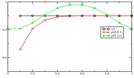
In order to study the queueing system given by our PSRA process we set a service time 𝑇 and define the instant traffic intensity 𝜚(𝜎, 𝑡) = 𝐸(𝑛(𝑡, 𝑡 + 𝑇 )). In fig. 2.3 and table 2.2 we report numerical results for the convergence of 𝜚(𝜎, 𝑡) to 𝜆𝑇 , granted by lemma 2.2.3. For simplicity we consider 𝜉 Gaussian, and 𝜆 = 1. In this case 𝜚(𝜎, 𝑡) converges as soon as 𝜎 gets close to 1. 𝜎 𝑇 𝜚(𝜎, 0) 𝜚(𝜎, 0.1) 𝜚(𝜎, 0.2) 𝜚(𝜎, 0.3)) 𝜚(𝜎, 0.4)) .2 .9 0.808534 0.808534 0.850089 0.907951 0.954826 .3 .9 0.868214 0.868214 0.88048 0.900153 0.919615 .4 .9 0.892048 0.892048 0.895086 0.900001 0.904914 .5 .9 0.898654 0.898654 0.899168 0.9 0.900832 .6 .9 0.899847 0.899847 0.899905 0.9 0.900095 .7 .9 0.899988 0.899988 0.899993 0.9 0.900007 .8 .9 0.899999 0.899999 0.9 0.9 0.9 .9 .9 0.9 0.9 0.9 0.9 0.9 1. .9 0.9 0.9 0.9 0.9 0.9 𝜎 𝑇 𝜚(𝜎, 0.5) 𝜚(𝜎, 0.6) 𝜚(𝜎, 0.7) 𝜚(𝜎, 0.8) 𝜚(𝜎, 0.9) .2 .9 0.9786 0.9786 0.954826 0.907951 0.850089 .3 .9 0.931537 0.931537 0.919615 0.900153 0.88048 .4 .9 0.907951 0.907951 0.904914 0.900001 0.895086 .5 .9 0.901346 0.901346 0.900832 0.9 0.899168 .6 .9 0.900153 0.900153 0.900095 0.9 0.899905 .7 .9 0.900012 0.900012 0.900007 0.9 0.899993 .8 .9 0.900001 0.900001 0.9 0.9 0.9 .9 .9 0.9 0.9 0.9 0.9 0.9 1. .9 0.9 0.9 0.9 0.9 0.9 Table 2.2:

(26)

0 0.2 0.4 0.6 0.8 1 0.6 0.8 1 λT ρ(σ,0.1) ρ(0.2,t)

Figure 2.3: Behavior of the function 𝜚(𝜎, 𝑡). On the 𝑥 axis we have time 𝑡 for 𝜚(0.2, 𝑡) and standard deviation 𝜎 for 𝜚(𝜎, 0.1).

We want to compare the average queue size in 𝑀/𝐷/1 queueing system (Poisson arrivals) with the 𝐺/𝐷/1 queueing system in which the arrivals are described in terms of PSRA. It is well known, see e.g.[7], that the stationary probabilities for the discrete time 𝐺/𝐷/1 queueing system are given by

𝑃0 = (𝑃0+ 𝑃1)𝑄0 .. . 𝑃𝑛= 𝑃0𝑄𝑛+ 𝑛+1 ∑︁ 𝑘=1 𝑃𝑘𝑄𝑛−𝑘+1 .. . (3.1)

where 𝑄𝑛 is the probability to have n arrivals in a service time slot. The corresponding generating function is given by

𝑃 (𝑧) = 𝑃0(1 − 𝑧)

1 −_𝑄(𝑧)𝑧 (3.2)

where

𝑃0= 1 − 𝜚 (3.3)

In the case of Poisson arrivals with traffic intensity 𝜚, 𝑄(𝑧) = 𝑞(𝑧) = exp(𝜚(𝑧 − 1)). Denoting by 𝑁 the average queue size, after straightforward computations we get

𝑃′(𝑧)⃒⃒

𝑧=1= 𝑁 =

𝜚(2 − 𝜚)

2(1 − 𝜚) (3.4)

Consider now the PSRA process. In this case we can try to compute (3.2) by means of the generating function (2.15). This is obviously an approximation, since the generating

(27)

2.3. QUEUEING SYSTEMS WITH PSRA PROCESS: INDEPENDENCE APPROXIMATION 17

function (3.2) is obtained under the hypothesis that the number of arrivals in subsequent slots are independent variables. Indeed this is not the case for PSRA arrivals, as it has been shown in Section 2. However, assuming that such independence we neglect possible effects of autocorrelation, then we have that 𝑄(𝑧) = 𝑞(𝜎)(𝑧). Now we employ the boundary condition 𝑃 (𝑧)|_𝑧=1= 1 and l’H^opital rule, also using the fact that 𝑞(𝜎)_(𝑧)⃒

⃒ 𝑧=1= 1, we find that 𝑃0 = 1 − ∑︁ 𝑖∈Z 𝑝𝑖(𝑡, 𝑡 + 𝑇 ) (3.5)

Now denoting by 𝑁 (𝜎, 𝑡) the average queue size and applying l’H^opital rule we get

𝑁 (𝜎, 𝑡) = 𝑃′(𝑧)⃒⃒ 𝑧=1= 𝑧𝑞(𝜎)(𝑧)𝑞𝑧𝑧(𝜎)(𝑧) − 2(︀𝑧𝑞𝑧(𝜎)(𝑧) − 𝑞(𝜎)𝑧 (𝑧) )︀ (︀𝑞(𝜎)𝑧 (𝑧) − 𝑧𝑞𝑧(𝜎)(𝑧))︀𝑞𝑧(𝜎)(𝑧) ⃒ ⃒ ⃒ ⃒ ⃒ 𝑧=1 (3.6) where 𝑞_𝑧(𝜎)(𝑧) =∏︁ 𝑖∈Z (1 + (𝑧 − 1)𝑝𝑖(𝑡, 𝑡 + 𝑇 )) ∑︁ 𝑖∈Z 𝑝𝑖(𝑡, 𝑡 + 𝑇 ) 1 + (𝑧 − 1)𝑝𝑖(𝑡, 𝑡 + 𝑇 ) 𝑞_𝑧𝑧(𝜎)(𝑧) =∏︁ 𝑖∈Z (1 + (𝑧 − 1)𝑝𝑖(𝑡, 𝑡 + 𝑇 )) ∑︁ 𝑘̸=𝑙 𝑘,𝑙∈Z 𝑝𝑘(𝑡, 𝑡 + 𝑇 )𝑝𝑙(𝑡, 𝑡 + 𝑇 ) (1 + (𝑧 − 1)𝑝𝑘(𝑡, 𝑡 + 𝑇 ))(1 + (𝑧 − 1)𝑝𝑙(𝑡, 𝑡 + 𝑇 ))

After few calculations we find

𝑁 (𝜎, 𝑡) = 2 ∑︀ 𝑖∈Z𝑝𝑖(𝑡, 𝑡 + 𝑇 ) − ( ∑︀ 𝑖∈Z𝑝𝑖(𝑡, 𝑡 + 𝑇 ))2− ∑︀ 𝑖∈Z𝑝2𝑖(𝑡, 𝑡 + 𝑇 ) 2(1 −∑︀ 𝑖∈Z𝑝𝑖(𝑡, 𝑡 + 𝑇 )) (3.7)

In order to give a complete description of our 𝐺𝐼/𝐷/1 queueing system in which the arrivals are described in terms of PSRA, we can find the stationary probability distributions 𝑃𝑛. We now consider (3.2). Using (3.5) and (2.15), we can rewrite (3.2) as

𝑃 (𝑧) = (1 − ∑︀ 𝑖∈Z𝑝𝑖(𝑡, 𝑡 + 𝑇 ))(1 − 𝑧) 1 −∏︀ 𝑧 𝑖∈Z(1+(𝑧−1)𝑝𝑖(𝑡,𝑡+𝑇 )) (3.8) Note that ⃒ ⃒ ⃒ ⃒ 𝑧 ∏︀ 𝑖∈Z(1 + (𝑧 − 1)𝑝𝑖(𝑡, 𝑡 + 𝑇 )) ⃒ ⃒ ⃒ ⃒ < 1 (3.9)

(28)

Therefore, 𝑃 (𝑧) = 𝑃0(1 − 𝑧) ∞ ∑︁ 𝑘=0 𝑧𝑘 (︀∏︀ 𝑖∈Z(1 + (𝑧 − 1)𝑝𝑖(𝑡, 𝑡 + 𝑇 )) )︀𝑘 = 𝑃0(1 − 𝑧) ∞ ∑︁ 𝑘=0 𝑧𝑘∏︁ 𝑖∈Z 1 (1 − (1 − 𝑧)𝑝𝑖(𝑡, 𝑡 + 𝑇 )))𝑘 = 𝑃0(1 − 𝑧) ∞ ∑︁ 𝑘=0 𝑧𝑘∏︁ 𝑖∈Z ∞ ∑︁ 𝑙=0 (︂𝑙 + 𝑘 − 1 𝑙 )︂ ((1 − 𝑧)𝑝𝑖(𝑡, 𝑡 + 𝑇 ))𝑙 = 𝑃0(1 − 𝑧) ∞ ∑︁ 𝑘=0 𝑧𝑘 ∞ ∑︁ 𝑙=0 (︂𝑙 + 𝑘 − 1 𝑙 )︂ (1 − 𝑧)𝑙∏︁ 𝑖∈Z (𝑝𝑖(𝑡, 𝑡 + 𝑇 ))𝑙 = 𝑃0(1 − 𝑧) ∞ ∑︁ 𝑘=0 𝑧𝑘 ∞ ∑︁ 𝑙=0 (︂𝑙 + 𝑘 − 1 𝑙 )︂ 𝑙 ∑︁ 𝑗=0 (︂ 𝑙 𝑗 )︂ 𝑧𝑗(−1)𝑗exp {︃ 𝑙∑︁ 𝑖∈Z log 𝑝𝑖(𝑡, 𝑡 + 𝑇 ) }︃ = 𝑃0(1 − 𝑧) ∞ ∑︁ 𝑘=0 ∞ ∑︁ 𝑙=0 (︂𝑙 + 𝑘 − 1 𝑙 )︂ 𝑙 ∑︁ 𝑗=0 (︂ 𝑙 𝑗 )︂ (−1)𝑗exp {︃ 𝑙∑︁ 𝑖∈Z log 𝑝𝑖(𝑡, 𝑡 + 𝑇 ) }︃ 𝑧𝑘+𝑗 = 𝑃0(1 − 𝑧) ∞ ∑︁ 𝑙=0 𝑙 ∑︁ 𝑗=0 ∞ ∑︁ 𝑛=𝑗 (︂𝑙 + 𝑛 − 𝑗 − 1 𝑙 )︂(︂ 𝑙 𝑗 )︂ (−1)𝑗exp {︃ 𝑙∑︁ 𝑖∈Z log 𝑝𝑖(𝑡, 𝑡 + 𝑇 ) }︃ 𝑧𝑛 = 𝑃0(1 − 𝑧) ∞ ∑︁ 𝑛=0 ∞ ∑︁ 𝑙=0 𝑛∧𝑙 ∑︁ 𝑗=0 (︂𝑙 + 𝑛 − 𝑗 − 1 𝑙 )︂(︂ 𝑙 𝑗 )︂ (−1)𝑗exp {︃ 𝑙∑︁ 𝑖∈Z log 𝑝𝑖(𝑡, 𝑡 + 𝑇 ) }︃ 𝑧𝑛 = 𝑃0 ∞ ∑︁ 𝑛=0 ∞ ∑︁ 𝑙=0 𝑛∧𝑙 ∑︁ 𝑗=0 (︂𝑙 + 𝑛 − 𝑗 − 1 𝑙 )︂(︂ 𝑙 𝑗 )︂ (−1)𝑗exp {︃ 𝑙∑︁ 𝑖∈Z log 𝑝𝑖(𝑡, 𝑡 + 𝑇 ) }︃ 𝑧𝑛− − 𝑃0 ∞ ∑︁ 𝑛=0 ∞ ∑︁ 𝑙=0 𝑛∧𝑙 ∑︁ 𝑗=0 (︂𝑙 + 𝑛 − 𝑗 − 1 𝑙 )︂(︂ 𝑙 𝑗 )︂ (−1)𝑗exp {︃ 𝑙∑︁ 𝑖∈Z log 𝑝𝑖(𝑡, 𝑡 + 𝑇 ) }︃ 𝑧𝑛+1 = 𝑃0 ∞ ∑︁ 𝑛=0 ∞ ∑︁ 𝑙=0 𝑛∧𝑙 ∑︁ 𝑗=0 (︂𝑙 + 𝑛 − 𝑗 − 1 𝑙 )︂(︂ 𝑙 𝑗 )︂ (−1)𝑗exp {︃ 𝑙∑︁ 𝑖∈Z log 𝑝𝑖(𝑡, 𝑡 + 𝑇 ) }︃ 𝑧𝑛− − 𝑃0 ∞ ∑︁ 𝑛=1 ∞ ∑︁ 𝑙=0 (𝑛−1)∧𝑙 ∑︁ 𝑗=0 (︂𝑙 + 𝑛 − 𝑗 − 2 𝑙 )︂(︂ 𝑙 𝑗 )︂ (−1)𝑗exp {︃ 𝑙∑︁ 𝑖∈Z log 𝑝𝑖(𝑡, 𝑡 + 𝑇 ) }︃ 𝑧𝑛

Hence we expand 𝑃 (𝑧) as a power series in 𝑧 and consequently we obtain an exact result for 𝑃𝑛, 𝑃𝑛= (1 − ∑︁ 𝑖∈Z 𝑝𝑖(𝑡, 𝑡 + 𝑇 )) ∞ ∑︁ 𝑙=0 𝑛∧𝑙 ∑︁ 𝑗=0 (︂𝑙 + 𝑛 − 𝑗 − 1 𝑙 )︂(︂ 𝑙 𝑗 )︂ (−1)𝑗exp {︃ 𝑙∑︁ 𝑖∈Z log 𝑝𝑖(𝑡, 𝑡 + 𝑇 ) }︃ − − (1 −∑︁ 𝑖∈Z 𝑝𝑖(𝑡, 𝑡 + 𝑇 )) ∞ ∑︁ 𝑙=0 (𝑛−1)∧𝑙 ∑︁ 𝑗=0 (︂𝑙 + 𝑛 − 𝑗 − 2 𝑙 )︂(︂ 𝑙 𝑗 )︂ (−1)𝑗exp {︃ 𝑙∑︁ 𝑖∈Z log 𝑝𝑖(𝑡, 𝑡 + 𝑇 ) }︃

(29)

2.4. NUMERICAL RESULTS 19

Note that, it is well known the steady state probability distribution 𝑃𝑛 for 𝑀/𝐷/1 (see e.g. [6]) queueing system is given by

𝑃𝑛= (1 − 𝜚) {︃ _𝑛 ∑︁ 𝑘=0 (−1)𝑛−𝑘𝑒𝑘𝜚(𝑘𝜚) 𝑛−𝑘 (𝑛 − 𝑘)! − 𝑛−1 ∑︁ 𝑘=0 (−1)𝑛−𝑘−1𝑒𝑘𝜚 (𝑘𝜚) 𝑛−𝑘−1 (𝑛 − 𝑘 − 1)! }︃ (3.10)

For 𝜎 large 𝑁 (𝜎, 𝑡) becomes independent of 𝑡, and it converges to 𝑁 by (2.23). Table 2.3 shows that for Gaussian 𝜉 and 𝜆 = 1 the convergence is quite fast.

𝜎 𝑇 𝑁 (𝜎, 0) 𝑁 (𝜎, 0.1) 𝑁 (𝜎, 0.2) 𝑁 (𝜎, 0.3) 𝑁 (𝜎, 0.4) 𝑁 (𝜎, 0.5) .1 .9 0.89105 0.89105 1.00493 1.04024 1.02267 1.00905 .2 .9 1.61425 1.61425 1.58187 1.51872 1.42902 1.32201 .3 .9 2.26812 2.26812 2.21399 2.10656 1.95949 1.83453 .4 .9 2.75253 2.75253 2.68673 2.57205 2.44587 2.36133 .5 .9 3.03548 3.03548 2.9955 2.92993 2.86327 2.82151 .6 .9 3.24502 3.24502 3.23019 3.20614 3.18205 3.16714 .7 .9 3.43207 3.43207 3.42809 3.42165 3.41521 3.41123 .8 .9 3.59488 3.59488 3.59405 3.5927 3.59134 3.59051 .9 .9 3.73131 3.73131 3.73117 3.73094 3.73071 3.73056 1. .9 3.84462 3.84462 3.8446 3.84457 3.84454 3.84452 𝜎 𝑇 𝑁 (𝜎, 0.6) 𝑁 (𝜎, 0.7) 𝑁 (𝜎, 0.8) 𝑁 (𝜎, 0.9) 𝑁 (𝜎, 1) .1 .9 1.00905 1.02267 1.04024 1.00493 0.89105 .2 .9 1.32201 1.42902 1.51872 1.58187 1.61425 .3 .9 1.83453 1.95949 2.10656 2.21399 2.26812 .4 .9 2.36133 2.44587 2.57205 2.68673 2.75253 .5 .9 2.82151 2.86327 2.92993 2.9955 3.03548 .6 .9 3.16714 3.18205 3.20614 3.23019 3.24502 .7 .9 3.41123 3.41521 3.42165 3.42809 3.43207 .8 .9 3.59051 3.59134 3.5927 3.59405 3.59488 .9 .9 3.73056 3.73071 3.73094 3.73117 3.73131 1. .9 3.84452 3.84454 3.84457 3.8446 3.84462 Table 2.3:

2.4 Numerical results

In the previous section we have computed the average queue size for the 𝐺/𝐷/1 queueing system in which the arrivals are described in terms of PSRA under the hypothesis that the number of arrivals in subsequent slots are independent variables. and we have remembered the formula for average queue size 𝑀/𝐷/1 queueing system. In this section we compare the PSRA average queue size 𝑁 (𝜎, 𝑡) obtained by numerical simulations to (3.7) and (3.4). We recall that (3.7) is obtained assuming the independence of number of arrivals in different time slots; (3.4) is the length of the queue for Poissonian arrivals. The numerical results can be found in table 2.4. In this table we can compare the values of average queue obtained by formula (3.4), (3.7) and simulation, for low traffic intensity (𝜚 = 0.5) and for heavy traffic intensity (𝜚 = 0.9)

(30)

𝜎 𝑇 𝑁 (3.3) 𝑁 (3.4) 𝑁 (𝑠𝑖𝑚) 0.1 0.5 0.75 0.5 0.4963 0.5 0.5 0.75 0.614554 0.5096 1 0.5 0.75 0.680202 0.5618 2 0.5 0.75 0.71483 0.6173 3 0.5 0.75 0.726519 0.6481 4 0.5 0.75 0.732381 0.6621 5 0.5 0.75 0.735901 0.6787 6 0.5 0.75 0.738249 0.6821 7 0.5 0.75 0.739927 0.6873 8 0.5 0.75 0.741186 0.6948 9 0.5 0.75 0.742165 0.6974 10 0.5 0.75 0.742949 0.7078 𝜎 𝑇 𝑁 (3.3) 𝑁 (3.4) 𝑁 (𝑠𝑖𝑚) 0.1 0.9 4.95 1.00905 0.9153 0.5 0.9 4.95 2.8215 1.2258 1. 0.9 4.95 3.84452 1.5004 2. 0.9 4.95 4.38353 1.834 3. 0.9 4.95 4.57059 2.0145 4. 0.9 4.95 4.66498 2.2124 5. 0.9 4.95 4.72181 2.3278 6. 0.9 4.95 4.75976 2.4414 7. 0.9 4.95 4.7869 2.555 8. 0.9 4.95 4.80726 2.6249 9. 0.9 4.95 4.8231 2.7232 10. 0.9 4.95 4.83583 2.8007 Table 2.4:

In figure 2.4 𝑁 (𝜎, 𝑡) is plotted as a function of 𝜎, for different values of 𝜚 = 0.5, 0.7, 0.9, and 𝑡 = 0.5. The dotted straight lines represent 𝑁 obtained by (3.4) for different values of 𝜚. As we can see from the graph, values of 𝑁 (𝜎, 𝑡 = 0.5) for fixed 𝜚 given by (3.7) are larger than the corresponding ones obtained by simulation. This is due to the fact that we neglected the (negative) autocorrelations. Moreover, while for small 𝜚 (say 𝜚 ≤ 0.6) approximation (3.7) gives relatively good results, the overestimate becomes very important when 𝜚 increases.

2.5 Queueing systems with PSRA process: autocorrelated

ar-rivals

As it is clear from the results of the previous section, neglecting the autocorrelation the estimate of the average queue length is grossly overestimated in the interesting cases. If we want to describe the system only by the length of the queue, the presence of autocorrelation implies the loss of Markov property. In this section we show that if we enlarge suitably the state space we may keep the Markov property, and describe completely the autocorrelation. With this description some interesting features of the system are clarified, but at the moment we are able to compute explicitly the quantities of interest with some approximations. Such approximations, however, turn out to give almost negligible errors.

To simplify the analytical treatment of the system, we will consider from now on densities 𝑓_𝜉(𝜎)(𝑡) of the random i.i.d. variables 𝜉𝑖 that are compact support, i.e. such that 𝑓_𝜉(𝜎)(𝑡) = 0 for 𝑡 > 𝐿 for some 𝐿 < ∞. We are setting 𝜆 = 1, and we take 𝐿 ∈ N. This implies that at a certain discrete time 𝑗 the 𝑖’th user is certainly arrived to the system for all 𝑖 ≤ 𝑗 − 𝐿, while for all 𝑖 ≥ 𝑗 + 𝐿 it is certainly not yet arrived. Hence to completely describe the state of the system we have to specify, beside the number 𝑛 of users waiting in queue right before the service at time 𝑗 is delivered, also a finite set 𝐼𝑗 of 𝑖’s, 𝐼𝑗 ⊂ {𝑗 − 𝐿 + 1, ..., 𝑗 + 𝐿 − 1}, that are the users that are already arrived at the service at time 𝑗. Note that the users in the set 𝐼𝑗 are not necessarily already served at time 𝑗, or, in other words, the set 𝐼𝑗 is the set of the users with indices in {𝑗 − 𝐿 + 1, ..., 𝑗 + 𝐿 − 1} that are in the queue at time 𝑗, or that are already served at time 𝑗. Note also that 0 ≤ |𝐼𝑗| ≤ 2𝐿 − 1. Finally, we want to outline that due to the independence of the 𝜉’s 𝐼𝑗+𝑖 is independent of 𝐼𝑗 for all 𝑖 ≥ 2𝐿.

(31)

2.5. QUEUEING SYSTEMS WITH PSRA PROCESS: AUTOCORRELATED ARRIVALS 21 A A A A A A A A A A A A 0 0.5 1 1.5 2 2.5 3 3.5 4 4.5 5 5.5 6 6.5 7 7.5 8 8.5 9 9.5 10 σ 0 0.5 1 1.5 2 2.5 3 3.5 4 4.5 5 5.5 N( σ, t) ρ=0.9 (3.4) ρ=0.9 (3.7) ρ=0.9 (Sim) A A ρ=0.7 (3.4) ρ=0.7 (3.7) ρ=0.7 (Sim) ρ=0.5 (3.4) ρ=0.5 (3.7) ρ=0.5 (Sim)

Figure 2.4: Behavior of the function 𝑁 (𝜎, 0.5), for different values of 𝜚. Dotted lines re-fer to Poisson arrivals, continuous lines rere-fer to approximation (3.7), dashed lines rere-fer to simulations.

We will treat first the case 𝜚 = 1, or in other words, the case 𝜆 = 𝑇 = 1 in (2.15). This special case is important for several reasons. First, we will prove that for PSRA arrivals the system has a finite average queue length, showing that, even if the PSRA process tends in distribution to the Poisson process, for finite variance of the 𝜉’s the two systems are deeply different. Second, we will show that in the 𝜚 = 1 case there is a conserved quantity in the system, when the stationary distribution is reached. Third, it is possible, using an interest interpretation of the system in terms of Fermi statistics, to compute the (very long) times needed to the system to reach the stationary distribution. Fourth, and maybe more important, on the basis of the computation of this relaxation times it is possible to approximate efficiently the distribution of the length of the queue even for 𝜚 < 1.

Hence, we fix 𝜚 = 1 and we start from the obvious relation

𝑛(𝑗 + 1) = 𝑛(𝑗) − (1 − 𝛿_𝑛(𝑗)0) + 𝑚(𝑗) (5.1) where 𝑛(𝑗) is the length of the queue immediately before the service at time 𝑗, 𝑚(𝑗) is the number of users arrived in the time slot [𝑗, 𝑗 + 1), and the term (1 − 𝛿𝑛(𝑗)0) indicates the fact that if there is some user in the queue at time 𝑗, i.e. 𝑛(𝑗) > 0, the first of the queue is served, while if 𝑛(𝑗) = 0 then 𝑛(𝑗 + 1) = 𝑚(𝑗).

Now we observe that with our notations we can write

𝑚(𝑗) = |𝐼𝑗+1| − |𝐼𝑗| + 1 (5.2)

This relation can be shown as follows: the total number 𝑛𝑎(𝑗) of users arrived to the service from a certain fixed time, say from time 1, to time 𝑗, is obviously 𝑛𝑎(𝑗) = 𝑗 − 𝐿 + |𝐼𝑗|, because all the users 𝑘 up to user 𝑗 − 𝐿’th are already arrived, due to the compactness of the support of 𝑓_𝜉(𝜎)(𝑡), while for 𝑘 > 𝑗 − 𝐿 the number of arrived users is |𝐼𝑗| by definition. Hence 𝑚(𝑗) = 𝑛𝑎(𝑗 + 1) − 𝑛𝑎(𝑗) = 𝑗 + 1 − 𝐿 + |𝐼𝑗+1| − 𝑗 + 𝐿 − |𝐼𝑗| = |𝐼𝑗+1| − |𝐼𝑗| + 1. Putting (5.2) into(5.1) we obtain

(32)

This relation shows that the quantity 𝛼(𝑗) = 𝑛(𝑗) − |𝐼𝑗| is constant during a busy period, and it increases by 1 at the end of each busy period. This implies that the stationary distribution is reached once 𝛼 > 0. If the initial value of 𝛼 is strictly positive, the value 𝑛(𝑗) = 0 is never realized, and then 𝛼 remains constant and

𝑁 = 𝐸(𝑛) = 𝛼 + 𝐸(|𝐼|) (5.4)

If the initial value of 𝛼 is 0 or it is negative, a sequence of busy periods is realized, giving in the end the value 𝛼 = 1, and the expected queue length 𝑁 = 𝐸(𝑛) = 1 + 𝐸(|𝐼|). Once the stationary value of 𝛼 > 0 is reached, the probability distribution of 𝑛 is given by

𝑃𝑘= 𝑃 (𝑛 = 𝑘) = 𝑃 (|𝐼| = 𝑘 − 𝛼) (5.5)

giving the obvious result that 𝑘 ≥ 𝛼. The explicit expression of the 𝑃𝑘 depends therefore from the distribution of the |𝐼|’s, and hence from the details of 𝑓_𝜉(𝜎)(𝑡). This solves completely the stationary problem in the 𝜚 = 1 case. For application to the air traffic, however, it could be also interesting to study some non stationary features of the system: in particular we want to compute the probability to pass from some negative value of 𝛼 to the following value 𝛼 + 1. These quantities are interesting in this 𝜚 = 1 case because if the probability to reach the state 𝑛 = 0 for a given 𝛼 ≤ 0 is much smaller that the inverse of the number of operation in a single day of traffic, it is very likely that the system remains on states 𝑛 > 0. These probability to jump from a definite value of 𝛼 to the following one are important also in the description of the 𝜚 < 1 case, as it will be explained below.

Hence suppose that at time 𝑗 the system is in the state 𝑛(𝑗) = 0, with a given value of 𝛼 < 0. Call 𝑡(𝛼) the quantity such that 𝑛(𝑗 + 𝑖) > 0 for all 0 < 𝑖 < 𝑡(𝛼), and 𝑛(𝑗 + 𝑡(𝛼)) = 0. 𝑡(𝛼) is therefore the length of the busy period with starting value 𝛼. We are interested to the quantities 𝑇 (𝛼) = 𝐸(𝑡(𝛼)). By the definition of 𝛼 we have that |𝐼𝑗| = −𝛼 + 1 and that the instant 𝑗 + 𝑡(𝛼) is the first instant after 𝑗 in which |𝐼_{𝑗+𝑡(𝛼)}| = −𝛼, having |𝐼𝑗+𝑖| > −𝛼 for all 0 < 𝑖 < 𝑡(𝛼). To compute 𝑇 (𝛼) we should evaluate the probability 𝑃 (|𝐼𝑗+𝑖| = −𝛼

⃒

⃒|𝐼_𝑗| = −𝛼 + 1). This probability are however hard to compute due to the conditioning. Here we introduce our approximation: we will measure 𝑇 (𝛼) in terms of

𝑇 (𝛼) ≈ 1

𝑃 (|𝐼| = −𝛼) (5.6)

i.e. we neglect the conditioning. This approximation is reasonable for 𝛼 such that 𝑃 (|𝐼| = −𝛼) ≪ _2𝐿1 : in these cases we have to expect that the probability to have 𝑃 (|𝐼𝑗+𝑖| = −𝛼

⃒ ⃒|𝐼𝑗| = −𝛼 + 1) for 𝑖 < 2𝐿 is very small, and since 𝐼𝑗+𝑖 is independent of 𝐼𝑗 for the greater values of 𝑖, that gives the bigger contribution to 𝑇 (𝛼), we have that the conditioning is almost ineffective. On the other side, for 𝛼 such that 𝑃 (|𝐼| = −𝛼) ≥ _2𝐿1 we have to expect a gross underestimate of 𝑃 (|𝐼𝑗+𝑖| = −𝛼

⃒

⃒|𝐼𝑗| = −𝛼 + 1), and therefore a gross overestimate of 𝑇 (𝛼). We will return on this point later.

We want now to compute explicitly 𝑃 (|𝐼| = −𝛼). We will write general formulas, valid for any density 𝑓_𝜉(𝜎)(𝑡), and we will also consider a concrete probability distribution for the delays 𝜉, namely the case of 𝑓_𝜉(𝜎)(𝑡) uniform in [−𝐿, 𝐿], in which many computations may be carried out explicitly.

By straightforward computations one can see that 𝑃 (|𝐼| = 0) = 𝐿−1 ∏︁ 𝑖=−𝐿+1 (1 − 𝐹𝜉(𝑖)) = (2𝐿)! (2𝐿)2𝐿 ≈ 𝑒 −2𝐿√_4𝜋𝐿 _(5.7)

(33)

2.5. QUEUEING SYSTEMS WITH PSRA PROCESS: AUTOCORRELATED ARRIVALS 23

where the last approximation is valid for uniform 𝜉’s, using Stirling formula, and 𝑃 (|𝐼| = 𝑘) = 𝑃 (|𝐼| = 0) ∑︁ −𝐿+1≤𝑖1<𝑖2<...<𝑖𝑘≤𝐿−1 𝐹𝜉(𝑖1) 1 − 𝐹𝜉(𝑖1) ... 𝐹𝜉(𝑖𝑘) 1 − 𝐹𝜉(𝑖𝑘) = = 𝑃 (|𝐼| = 0) ∑︁ −𝐿+1≤𝑖1<𝑖2<...<𝑖𝑘≤𝐿−1 𝐿 − 𝑖1 𝐿 + 𝑖1 ...𝐿 − 𝑖𝑘 𝐿 + 𝑖𝑘 (5.8) where 𝐹𝜉(𝑡) is the probability distribution of the 𝜉’s, and the last equality is again valid for uniform distribution.

It is worthy to observe that (5.8) may be interpreted as the canonical partition function of a Fermi system with 2𝐿 energy level and 𝑘 particles, where the 𝑖-th level has energy log(𝐹𝜉(𝑖)) − log(1 − 𝐹𝜉(𝑖)). With this respect many computational techniques may be used in order to compute the probabilities 𝑃 (|𝐼| = 𝑘). Note that, in the approximation (5.6), once we are able to compute the quantities 𝑃 (|𝐼| = 𝑘) we know also the expected values 𝑇 (𝛼). Let us list here a couple of possible way to evaluate 𝑃 (|𝐼| = 𝑘) using the fact that, since it is possible to interpret it as a well known object in statistical mechanics, one can use computational results that are classical in that framework. The number of energy level, as mentioned above, is 2𝐿. In real traffic context one should expect that this value is of the order 20 or 30. One of the available approximation of the quantity 𝑃 (|𝐼| = 𝑘), i.e. the so called equivalence with the grand canonical ensemble, uses a method that is roughly speaking the Lagrange multipliers method, giving very good approximations for 2𝐿 large (see e.g. [20, chapter 5, section 53]. Since in our case 2𝐿 is not large enough to ensure the goodness of the approximation, it is much better to use an exact expression for 𝑃 (|𝐼| = 𝑘), due to Ginibre. For completeness, and for the fact that it is quoted in a very implicit sense in [43], we give the proof of this formula.

Calling 𝑤𝑖= _1−𝐹𝐹𝜉(𝑖)_𝜉_(𝑖), one can prove the following equality

𝑃 (|𝐼| = 𝑘) = 𝑘 ∑︁ 𝑙=0 ∑︁ 1≤𝑗1≤...≤𝑗𝑙 ∑︀ 𝑚 𝑗𝑚=𝑘 𝐶(𝑗1, ..., 𝑗𝑙) 𝑙 ∏︁ 𝑚=1 ∑︁ 𝑖 (𝑤𝑖)𝑗𝑚 (5.9) with 𝐶(𝑗1, ..., 𝑗𝑙) = 𝑃 (|𝐼| = 0) (−1)𝑘−𝑙 𝑗1...𝑗𝑙𝑚1!...𝑚𝑘! (5.10) where 𝑚𝑖 is the number of 𝑗’s equal to 𝑖. To prove (5.9) we observe that

𝑃 (|𝐼| = 𝑘) = 𝑃 (|𝐼| = 0)1 𝑘! 𝑑𝑘 𝑑𝑡𝑘 ∏︁ 𝑖 (1 + 𝑡𝑤𝑖) ⃒ ⃒ ⃒ ⃒ ⃒ 𝑡=0 The quantity∏︀

𝑖(1 + 𝑡𝑤𝑖) can be expanded in series as follows 1 𝑘! 𝑑𝑘 𝑑𝑡𝑘 ∏︁ 𝑖 (1 + 𝑡𝑤𝑖) ⃒ ⃒ ⃒ ⃒ ⃒ 𝑡=0 = 1 𝑘! 𝑑𝑘 𝑑𝑡𝑘𝑒 ∑︀ 𝑖log(1+𝑡𝑤𝑖) ⃒ ⃒ ⃒ ⃒ 𝑡=0 = 1 𝑘! 𝑑𝑘 𝑑𝑡𝑘𝑒 ∑︀ 𝑖 ∑︀𝑘 𝑗=1(−1)𝑗−1 (𝑡𝑤𝑖) 𝑗 𝑗 ⃒ ⃒ ⃒ ⃒ 𝑡=0 = = 1 𝑘! 𝑑𝑘 𝑑𝑡𝑘𝑒 ∑︀𝑘 𝑗=1(−1)𝑗−1 𝑡 𝑗 𝑗 ∑︀ 𝑖(𝑤𝑖)𝑗 ⃒ ⃒ ⃒ ⃒ 𝑡=0 = 1 𝑘! 𝑑𝑘 𝑑𝑡𝑘 𝑘 ∑︁ 𝑙=1 (∑︀𝑘 𝑗=1(−1)𝑗−1 𝑡 𝑗 𝑗 ∑︀ 𝑖(𝑤𝑖)𝑗)𝑙 𝑙! ⃒ ⃒ ⃒ ⃒ ⃒ 𝑡=0 =

(34)

= 𝑘 ∑︁ 𝑙=0 (−1)𝑘−𝑙 𝑙! ∑︁ 𝑗1,...,𝑗𝑙 ∑︀ 𝑚 𝑗𝑚=𝑘 𝑙 ∏︁ 𝑚=1 ∑︁ 𝑖 (𝑤𝑖)𝑗𝑚 𝑗𝑚 = 𝑘 ∑︁ 𝑙=0 (−1)𝑘−𝑙 𝑙! ∑︁ 1≤𝑗1≤...≤𝑗𝑙 ∑︀ 𝑚 𝑗𝑚=𝑘 𝑙 ∏︁ 𝑚=1 ∑︁ 𝑖 (𝑤𝑖)𝑗𝑚 𝑗𝑚 𝑙! 𝑚1!...𝑚𝑘! which is (5.9).

We conclude then the discussion of the 𝜚 = 1 case observing that in a concrete framework of air traffic, if we want to avoid to have lost slot but we want to keep the queue as short as possible we have to choose initial condition in such a way that 𝛼 is the smaller possible value such that 𝑇 (𝛼) > 𝐷, where 𝐷 is the number of operations in a day. This value of 𝛼 gives the corresponding value of the length of the queue using (5.4).

A simple observation allows us to give an estimate of the average length of the queue also when 𝜚 < 1. Let us suppose that we impose the condition 𝜚 < 1 keeping the time between two expected arrivals equal to the service time, but assuming that the arrivals are described by PSRA process with random deletion (see (2.16)), with probability of deletion equal to 1 − 𝜚. It is easy to realize that this corresponds to say that the value of 𝛼 has a probability 1 − 𝜚 to decrease by one. Hence we have this picture of our queueing system: the queue is described by a superposition of a slow varying process, the process that describes the value of 𝛼, and a fast varying process, the one describing the 𝑛 for fixed 𝛼. If we are able to compute the distribution probabilities of the values of 𝛼, we can evaluate the expected length of the queue (and even its distribution) by (5.4), weighted with the probabilities of the various values of 𝛼.

In the unconditioned approximation (5.6), the computation of the stationary probabilities 𝜋𝛼 of 𝛼 is a standard task of the theory of the birth-and-death processes: the evolution of 𝛼 is a discrete time birth-and-death process, with transition probabilities

𝑃𝛼,𝛼′ = ⎧ ⎪ ⎪ ⎪ ⎪ ⎨ ⎪ ⎪ ⎪ ⎪ ⎩ 1 − 𝜚 ≡ 𝜇𝛼 if 𝛼′ = 𝛼 − 1 𝑃 (|𝐼| = −𝛼) ≡ 𝜆𝛼 if 𝛼′ = 𝛼 + 1 1 − 𝜆𝛼− 𝜇𝛼 if 𝛼′ = 𝛼 0 otherwise

and boundary conditions 𝜇−𝐿+1= 𝜆0 = 0. We get the following linear system 𝜋−𝐿+1 = 𝜋−𝐿+1(1 − 𝜆−𝐿+1) + 𝜋−𝐿+2𝜇−𝐿+2 𝜋𝑖 = 𝜋𝑖−1𝜆𝑖−1+ 𝜋𝑖+1𝜇𝑖+1+ 𝜋𝑖(1 − 𝜆𝑖− 𝜇𝑖) − 𝐿 + 1 < 𝑖 < 0 𝜋0 = 𝜋−1𝜆−1+ 𝜋0(1 − 𝜇0) whose solution is 𝜋𝑖 = 𝜋−𝐿+1 𝑖 ∏︁ 𝑘=−𝐿+2 𝜆𝑘−1 𝜇𝑘

The stationary distribution 𝜋 is defined by the normalization condition∑︀

𝑖𝜋𝑖 = 1, then 𝜋−𝐿+1= 1 1 +∑︀0 𝑛=−𝐿+2 ∏︀𝑖 𝑘=−𝐿+2 𝜆𝑘−1 𝜇𝑘 (5.11)

This approximation is good for 1 − 𝜚 sufficiently small, because the probability to increase 𝛼 = −𝐿 + 1 is much bigger than the probability to decrease it, and at the same time the un-conditioned transition probabilities to increase 𝛼 when 𝛼 > −𝐿 + 1 are a good approximation of the actual transition probabilities.

(35)

2.6. CONCLUSIONS AND OPEN PROBLEMS 25

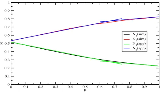
In the following figure we show the value of the expected length of the queue obtained by the formula

𝑁 =∑︁ 𝛼

𝜋𝛼(𝛼 + 𝐸𝛼(|𝐼|)) (5.12)

Note that 𝐸𝛼(|𝐼|) is 𝛼-dependent, because in its computation we neglect the terms with |𝐼| < −𝛼, since they do not contribute to the evolution of the process with that value of 𝛼. As it can be seen from the figure, the estimate of the average length of the queue is extremely near to the simulations, also for highly congested systems. In the figure we have shown for completeness also the (wrong, for high 𝜚) values of the length of the queue computed by means of formula (3.7), which neglects the autocorrelations.

0.85 0.86 0.87 0.88 0.89 0.9 0.91 0.92 0.93 0.94 0.95 0.96 0.97 0.98 0.99 1 1.01 ρ 0 1 2 3 4 5 6 7 8 9 N N(uncorr) N(sim) N(app)

Figure 2.5: The length of the queue for highly congested systems, computed by means of numerical simulations (red line) and our analytical approximation (blue line). It can be seen that the uncorrelated approximation (black line) obtained by formula (3.7) gives for these values of 𝜚 a gross overestimate. The simulations are run for a time sufficiently long to have fluctuations on the result negligible in the scale of the figure.

2.6 Conclusions and open problems

The main aim of this chapter is to study a stochastic process close to the Poisson process, but more suitable to describe the arrivals to a queueing systems when such arrivals are scheduled in advance, and some randomness is added to the schedule. We looked into this problem as an attempt to describe the congestion in air traffic systems, but the same construction can be used in different contexts.

We found some analytical results, in particular we showed that our process can be indistin-guishable from a Poisson process if one wants to study the distribution either of the number of arrivals or of the interarrival times in a time slot shorter than the standard deviation of the randomness imposed to the scheduled arrivals.

However we have shown that from the point of view of the resulting congestion, due to the autocorrelation of this stochastic process, the queueing properties of this model are quite