Analysis and mitigation of pupil discontinuities on adaptive optics performance

(1)

2018

Publication Year

2020-11-13T12:01:54Z

Acceptance in OA@INAF

Analysis and mitigation of pupil discontinuities on adaptive optics performance

Title

Schwartz, Noah; Sauvage, Jean-François; Correia, Carlos; Neichel, Benoit; Fusco,

Thierry; et al.

Authors

10.1117/12.2313129

DOI

http://hdl.handle.net/20.500.12386/28313

Handle

PROCEEDINGS OF SPIE

Series

10703

Number

(2)

PROCEEDINGS OF SPIE

SPIEDigitalLibrary.org/conference-proceedings-of-spie

Analysis and mitigation of pupil

discontinuities on adaptive optics

performance

Noah Schwartz, Jean-François Sauvage, Carlos

Correia, Benoit Neichel, Thierry Fusco, et al.

Noah Schwartz, Jean-François Sauvage, Carlos Correia, Benoit Neichel,

Thierry Fusco, Fernando Quiros-Pacheco, Kjetil Dohlen, Kacem El Hadi,

Guido Agapito, Niranjan Thatte, Fraser Clarke, "Analysis and mitigation of

pupil discontinuities on adaptive optics performance," Proc. SPIE 10703,

Adaptive Optics Systems VI, 1070322 (10 July 2018); doi:

10.1117/12.2313129

Event: SPIE Astronomical Telescopes + Instrumentation, 2018, Austin, Texas,

United States

(3)

Analysis and mitigation of pupil discontinuities on adaptive optics

performance

Noah Schwartz*

a

, Jean-François Sauvage

b

, Carlos Correia

c

, Benoit Neichel

c

, Thierry Fusco

b

,

Fernando Quiros-Pacheco

d

, Kjetil Dohlen

c

, Kacem El Hadi

c

, Guido Agapito

e

, Niranjan Thatte

f

,

Fraser Clarke

f

a

_{UK Astronomy Technology Centre, Blackford Hill, Edinburgh EH9 3HJ, United Kingdom;}

b

_{ONERA, 29 avenue de la Division Leclerc, 92322 Châtillon, France;}

c

_{LAM, Laboratoire}

d'Astrophysique de Marseille, Marseille, France;

d

GMTO Organization, 465 North Halstead St, Suite

250, Pasadena, CA 91107, USA;

e

INAF - Osservatorio Astrofisico di Arcetri, Largo E. Fermi 5,

50125 Firenze, Italy;

f

Dept. of Astrophysics, University of Oxford, Keble Road, Oxford, OX1 3RH,

United Kingdom;

ABSTRACT

As already noticed in other telescopes, the presence of large telescope spiders and of a segmented deformable mirror in an Adaptive Optics system leads to pupil fragmentation and may create phase discontinuities. On the ELT telescope, a typical effect is the differential piston, where all disconnected areas of the pupil create their own piston, unseen locally but drastically degrading the final image quality. The poor sensitivity of the Pyramid WFS to differential piston will lead to these modes been badly seen and therefore badly controlled by the adaptive optics (AO) loop. In close loop operation, differential pistons between segments will start to appear and settle around integer values of the average sensing wavelength. These additional differential pistons are artificially injected by the adaptive optics control loop but do not have any real physical origin, contrary to the Low Wind Effect.

In an attempt to reduce the impact of unwanted differential pistons that are injected by the AO loop, we propose a novel approach based on the pair-wise coupling of the actuators sitting on the edges of the deformable mirror segments. In this paper, we present the correction principle, its performance in nominal seeing condition, and its robustness relative to changing seeing conditions, wind speed and natural guide star magnitude. We show that the edge actuator coupling is a simple and robust solution and that the additional quadratic error relative to the reference case (i.e. no spiders) is of only 40 nm RMS, well within the requirements for HARMONI.

Keywords: Adaptive Optics, Optical Modelling, Pyramid Wavefront Sensing, Spiders, Differential Piston, ELT

1. INTRODUCTION

The secondary mirror unit of the European Extremely Large Telescope (ELT) is supported by six 50-cm wide spiders, providing the necessary stiffness to the structure while minimising the obstruction of the beam. The deformable quaternary mirror (M4) contains over 5000 actuators on a nearly hexagonal pattern. The reflective surface of M4 itself is composed of a segmented thin shell made of 6 discontinuous petals. This segmentation of the telescope pupil will create areas of phase isolated by the width of the spiders on the wavefront sensor (WFS) detector, breaking the spatial continuity of the wavefront data.

The poor sensitivity of the Pyramid WFS to differential piston will lead to badly seen and therefore nearly uncontrollable differential pistons between these areas. In close loop operation, differential pistons between segments will settle around integer values of the central sensing wavelength λWFS. The differential pistons typically range from one to tens of time the sensing wavelength and can vary rapidly over time depending on conditions.

*noah.schwartz@stfc.ac.uk; phone: +44 (0)131 668 8256

CCC code: 0277-786X/18/$18 · doi: 10.1117/12.2313129

Proc. of SPIE Vol. 10703 1070322-1 Downloaded From: https://www.spiedigitallibrary.org/conference-proceedings-of-spie on 8/9/2018

(4)

Even if the local piston (defined as the mean phase on a single segment of the pupil) does not impact the wavefront locally, the different pistons between each pupil segments will lead to extremely poor performance. In addition, aberrations created by atmospheric turbulence will naturally contain some differential piston between the segments. For badly seen modes with low associated energy (such as waffle), a typical approach is to put these modes in the null space of the direct modal and filter them out during the inversion process. Since the energy of these modes is negligible, the loss in performable is insignificant. However, the energy associated with differential piston is not negligible and these modes cannot be simply filtered out. This means that we cannot simply rely on the DM shape and remove the differential piston from each pupil segment because a large part of it is required to compensate for atmospheric turbulence. In an attempt to reduce the impact of unwanted differential pistons that are injected by the AO correction, we propose a novel approach based on the pair-wise coupling of the actuators sitting on the edges between the deformable mirror segments. In this paper, we first present the context of this study HARMONI, a visible and near-infrared integral field spectrograph providing the European Extremely Large Telescope. We then distinguish between two separate effects created by the pupil dislocation and the presence of spiders. The first one is the low wind effect and is out of the scope of this paper. The second is the island effect and will be the focus of the following sections. We first explain the principle of the edge actuator coupling and compare its performance to the reference case (i.e. no spiders). We then explore the robustness of this control strategy relative to changing atmospheric conditions, wind speed or natural guide star magnitude. We show that the edge actuator coupling is a simple and robust solution and that the additional quadratic error relative to the reference case (i.e. no spiders) is of only 40 nm RMS, well within the requirements for HARMONI.

2. CONTEXT AND NOMINAL PERFORMANCE 2.1 HARMONI and the ELT

HARMONI [1] is a visible and near-infrared integral field spectrograph providing the European Extremely Large Telescope (ELT) with its core spectroscopic capability. It will exploit the ELT’s scientific niche in its early years, starting at first light. To fully exploit the spatial resolution and collecting power gain of the ELT, HARMONI will rely on the telescope's adaptive M4 and M5 mirrors. Two different adaptive optics (AO) systems will be used enabling both high-performance combined with low sky coverage using bright natural guide stars (single-conjugate adaptive optics, SCAO) [2, 3] and medium performance combined with excellent sky coverage using 6 laser guide stars and faint natural guide stars for low-order correction (laser tomography adaptive optics, LTAO) [2, 4].

HARMONI will use ELT’s deformable quaternary mirror (M4) which contains over 5000 actuators positioned on a nearly hexagonal pattern. The average pitch between actuators is approximately 50 cm when projected onto the primary mirror (M1). M4 is composed of a segmented thin shell made of 6 discontinuous petals. The segments are discontinuous, but a common silicon carbide (SiC) reference body will ensure that actuators can be driven into position with a known absolute position. In addition, the secondary mirror unit of the ELT is supported by six 50-cm wide spiders, providing the necessary stiffness to the structure while minimising the obstruction of the beam. Such segmentation of the telescope pupil will create areas of phase isolated by the width of the spiders on the wavefront sensor (WFS) detector, breaking the spatial continuity of the wavefront data. HARMONI will be installed on the Nasmyth platform of the ELT. Its SCAO system will use a modulated Pyramid WFS (P-WFS). For more information on the SCAO system of HARMONI see related in this conference [5].

2.2 Nominal SCAO performance

The main requirement for the SCAO system of HARMONI is specified for median seeing conditions, at 30⁰ zenith angle, and for a bright natural reference star (magnitude 12 in R). The seeing conditions as per defined by ESO [6] are summarised in Table 1. It shows the equivalent Fried parameter (r0) for the nominal 30⁰ zenith angle, at 60⁰, and for different wavelengths. The wavefront sensing wavelength for HARMONI is defined in the I-band (i.e. centred on 750 nm). The Fried parameter in median seeing conditions, at this wavelength, and at 30⁰ zenith angle is 23.2 cm. It is important to note that r0 will be smaller than the spiders’ width for all seeing conditions, even for the most favourable quartile JQ1. To ensure larger r0, one would for example need to increase the wavelength. In the K-band (i.e. 2.2 μm) the Fried parameter is systematically larger than the spiders’ width even for the harshest turbulence conditions JQ4.

(5)

50 DO 50 D0 2 I f ...Reference Case l ir I I Ar

SCAO performance v_ spping

0

0 4 0.5 0.6 0.7 0.8 0.9

Seeing [arsec]

1.1 1 2

104 Reference Case: O.65aresec

Atmospheric Turbulence SCAO Correction

io2

0 1000 2000 3000 4000 5000

Iteration number

Table 1: Seeing conditions and Fried parameter (r0) at 30⁰ zenith angle for different wavelengths. The nominal case for the

HARMONI SCAO study is highlighted in bold.

λ Zenith Median JQ1 JQ2 JQ3 JQ4 Seeing [arcsec] 500 nm 0⁰ 0.65 0.44 0.57 0.73 1.04 r0 [cm] 750 nm 30⁰ 23.2 34.3 26.5 20.7 14.5 750 nm 60⁰ 10.3 15.2 11.7 9.1 6.4 1.6 μm 30⁰ 57.6 85.1 65.7 51.3 36.0 2.2 μm 30⁰ 84.4 124.7 96.3 75.2 52.8

The WFS for the SCAO system of HARMONI is a 100×100 pyramid WFS (P-WFS) running at 500 Hz. We use a classical integrator control with 2 frames delay:

𝑢𝑛+1= 𝑢𝑛− 𝑔𝑀𝑐𝑜𝑛𝑡𝑟𝑜𝑙𝑠𝑘

Where Mcontrol is the control matrix, g is the uniform scalar gain of the integrator, un is the DM control vector at time n, and sk is the slope vector. Mcontrol is calculated from the generalised pseudo-inverse of the interaction matrix. Instead of using a zonal approach (i.e. poke matrix) we use a modal approach using Karhunen-Loeve modes (re-orthonormalised over the ELT pupil and using the actual influence functions of M4). The number of modes we control in the AO loop is selected very coarsly to avoid any overshoot of the controlled modes while still minimising the fitting error. 4600 modes are controlled in weak seeing conditions (i.e. up to 0.85 arcsec) and 4000 modes are controlled above for stronger turbulence. Fine tunning of the number of modes and of the control law is out of the scope of this paper and will be done in a later stage of the project.

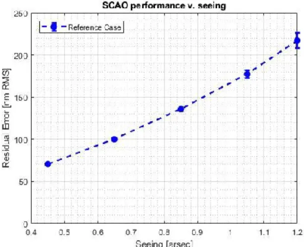
Figure 1: Reference SCAO performance: residual error as a function of seeing condition. The error bar represents the standard deviation of the results.

Figure 2: SCAO performance for the reference case as a function of loop iterations. Median seeing conditions,

modulation 3λ/D.

In the absence of spiders and using a continuous DM surface (the real M4 is composed of 6 optically disconnected segments that are physically connected through a common baseplate) we are able to evaluate the SCAO performance in an ideal scenario. This will serve as a reference case so that other more realistic scenarios can be benchmarked against this reference. Figure 1 shows the average pure SCAO residual error for the reference case. It only takes into account the fitting, servo-lag, aliasing, chromatic, and noise errors. No other errors (e.g. low-order optimisation loop, M1 co-phasing errors etc.) are taken into account. Using a very simple control strategy we are able to show good overall performance for the studied seeing conditions and very good stability of the residual error at convergence. For example, the pure-AO Strehl ratio in the K-band and at high flux is 92% (101 nm RMS residual error) for a seeing of 0.65 arcsec. Figure 2 shows the residual error as a function of iteration step for the reference case, a P-WFS modulation of 4λ/D, and a seeing of 0.65˝. The rapid convergence and the stability of the loop are clearly visible.

(6)

E

w

20

Turbulent phase [um] 5 10 15 m 25 30 35 40 0 0 20 Distance [m 30 40 o 5 4 T 3

3

2 c 1 ó v 0 m w-1 > < -2 -3 4

Atmospheric segment piston

2 3 4 5 Segment number 6 E

3 c

w E oi w ñ 0 c o w oi > Q 5 0

5 Segment piston: Atmosphere

Segment 1 Segment 2 Segment 3 Segment 4 Segment 5 Segment 6 1 2 3 Time [5]

Phase difference either side of spider

t

11,

1 2 3 Time [s] 5

2.3 Atmospheric differential piston

Figure 3: Example of atmospheric phase (in μm) with an average piston over the pupil set to 0. Segments are labelled from the far right and anti-clockwise.

Figure 4: Piston values integrated over each petal segment (in microns) corresponding to the phase in Figure 3. The total piston is set to zero.

Atmospheric turbulence will naturally produce differential piston between each of the six DM segments (often termed petals). Figure 3 shows an example of atmospheric phase in the pupil of the telescope in the presence of spiders (no AO correction). The global piston is set to zero. Figure 4 represents the average piston per segment for the phase presented Figure 3, and shows large natural variations ranging from ±4 μm in this particular example.

Differential piston between segments will evolve as the turbulence changes. Figure 5 shows an example of how the differential pistons of the turbulent atmosphere can evolve over time. It shows that the differential piston can be large (up to ±5 μm in this illustration) and that variations are slow with a typical evolution time over several seconds. The average wind speed in this particular example was set at 5.5 m/s.

Another important aspect to note is that the 50 cm spiders are larger than the coherence length of the atmosphere. This means that the phase on either side of the spiders will be decorrelated. From the phase spatial structure function:

𝐷𝜑(𝜌 ≪ 𝐿0) = 〈|𝜑𝑟− 𝜑𝑟+𝜌| 2

〉 = 6.88(𝑑 𝑟⁄ )₀ 5/3one can expect phase difference to be approximately 1 wave in median seeing conditions (for large distances the structure function will converge to 𝐷𝜑(𝜌 → ∞) = 2𝜎𝜑2) . Figure 6 shows the evolution of

the phase difference between 2 points in the pupil distant from 50 cm. It varies rapidly over time and can have large value (±1 μm in our example in median seeing conditions).

Figure 5: Evolution of atmospheric piston as a function

of time. Seeing of 1.05 arcsec at 30⁰ of zenith angle. Figure 6: Evolution of the different between phase points distant by the spider width (i.e. 50 cm).

3. IMPACT OF SUPPORT STRUCTURESAND PUPIL FRAGMENTATION

One of the major limiting factors to achieving the high performance presented in section 2.2 is imposed by the presence of discontinuities within the telescope pupil. The major source of these large gaps is created by the telescope’s spiders themselves, the second coming from the physical discontinuities created by the 6 unconnected M4 segments (i.e. the influence functions stop at the edge of the segments). The principle impact can be described as a combination of

(7)

p

differential piston, tip, and tilt between the wavefront in the different sections of the telescope’s pupil. In this paper we distinguish between two effects. The low wind effect [7, 8, and 9]: a combination of differential piston, tip, and tilt created by radiative cooling of the telescope spiders. The strength of the low wind effect will essentially depend on the height of the spiders. The second is the island effect [10]: a differential piston between the mirror segments created by the AO control loop (this is true for any badly seen modes (such as waffle) that will undergo amplification during the inversion/reconstruction). The strength of the island effect (IE) is mainly driven by the width of the telescope’s spiders, in our case 50 cm. They may in practice have similar impact on the point-spread function and correction quality, but arise from entirely different origins.

3.1 Low Wind Effect

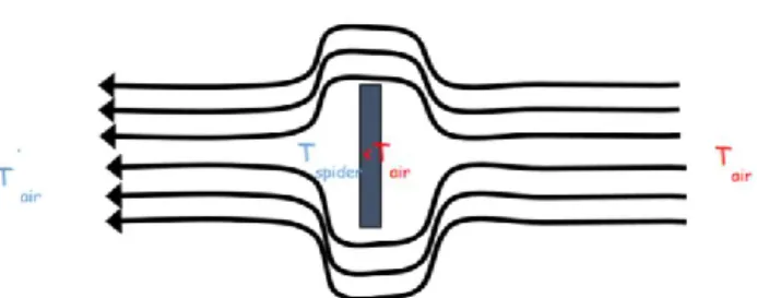
Low Wind Effect (LWE) aberrations are created by air temperature gradients at the level of the telescope spiders. The physical origin of the LWE is well explained [7, 11] by the radiative cooling of the telescope spiders, creating non-uniform air temperatures across the telescope pupil. The wavefront steps across the pupil are extremely sharp, defined by the spider arm. Figure 7 represent the wavefront map taken during on-sky measurements of commissioning number 4 [7] clearly showing piston, tip and tilt on each of the 4 quadrants. The LWE pattern (see Figure 8, right-hand side), is created by radiative transfer between the spider and the sky background, largely decreasing the temperature of the spider. The air coming on the spider has a higher temperature than the spider and therefore loses heat when crossing it (see Figure 8, right-hand side). The air after the spider has a decreased temperature. This temperature difference creates a temperature gradient between air on either side of the spider arm. As an example, a temperature difference of 1°C cumulated on a 1 m height is responsible for an optical path difference of 800 nm between each side of the spider. LWE generally appears in the absence or in very low wind conditions (hence the name) when convection is unable to produce an equal temperature throughout. The typical temporal evolution is greater than 1 s.

Figure 7: Wavefront aberration measured by ZELDA wavefront sensor of SPHERE, during on-sky measurement of commissioning 4 [7] showing piston,

tip and tilt on each of the 4 quadrants.

Figure 8: Scenario of the LWE: the radiative transfer decreases the temperature of the spider. Some heat exists between the air at temperature Tair and the spider

at Tspider, leading to a difference [7].

LWE was only recently successfully diagnosed on VLT/SPHERE [7] and a new mitigation strategy was recently proposed and implementer at the end of 2017, when a coating with low thermal (in the mid-infrared) emissivity was fixed to the spiders. This has been shown to dramatically reduce the LWE by a factor around 5 as a first approximation [11]. However this reduction needs to be quantified in the case of ELT instruments and in particular for HARMONI. In particular, on ELT the height of the spiders will be 5 times larger than on VLT. The solution proposed for VLT, applied on ELT will therefore leave a LWE residual on ELT of the order of magnitude of the uncorrected LWE on VLT which means around 1 micrometre.

3.2 Island Effect

The Island Effect (IE) on the other hand is a ‘non-physical’ effect in the sense that it is generated by the numerical AO control loop itself and not by any other real physical process. When the width of the spider is no longer negligible compared to the size of the sub-apertures (for HARMONI, the pixel size on the P-WFS detector is 37 cm), they will hide

(8)

3500 3000 2500 VI 2 i= C C w 1500 2000 1000 500 1000 2000 3000 Iteration number 4000 5000 Lona- exposure PSF -5 0 Angle [mas] 5

full rows of pixels. The spiders divide the measured wavefront slopes map into disconnected domains, with completely missing or corrupted measurements between them. In addition, since the segmented DM is matching the spider geometry, it is fully capable of creating discontinuous modes fitting the 6 petal geometry. Modes that are badly seen (and this is particularly true for differential pistons) or not sensed at all by the PWFS and that the DM is capable of producing will start to appear when the AO loop is closed. This differential piston between the mirror segments created by the AO control loop is often termed the Island Effect (IE). For SPHERE the IE is negligible since the VLT spiders are only 5 cm wide and the sub-apertures are 20 cm large. The sub-apertures are much greater than the gap and the spiders will only cause a slight reduction in flux.

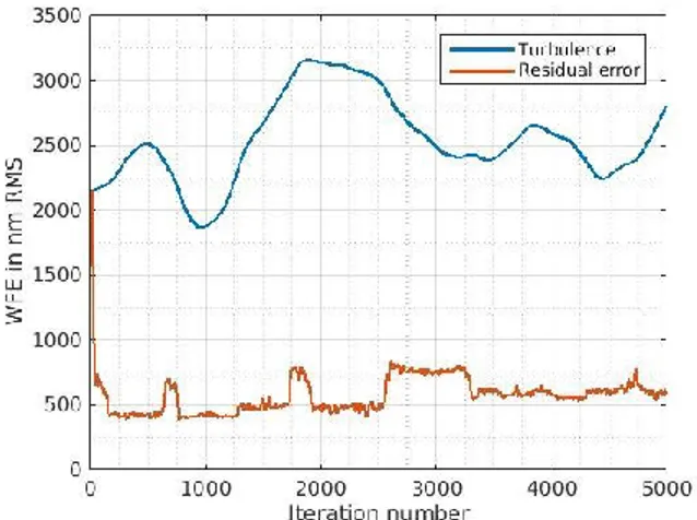
Figure 9 presents the evolution of the residual error as a function of time and shows the clear instability created by differential pistons. The modulation of the Pyramid WFS was set at 3λ/D. The SCAO performance is somewhat affected by the modulation diameter, but the main conclusions remain the same. The average performance after convergence is of the order of 570 nm RMS in median seeing (or a Strehl Ratio of 7% in the K-band) with instantaneous performance ranging between 400 and 800 nm RMS. An illustration of the obtained PSF is given in Figure 10. On top of the very poor average performance, the PSF appears to be split in two due to the IE.

Figure 9: SCAO performance in presence of spider - residual error as a function of time.

Figure 10: Example of PSF obtained in the presence of spiders in median seeing conditions.

3.3 Island Effect mitigation

Unlike the Shack-Hartmann, it has been shown [12] that the P-WFS is sensitive to the differential piston. From Vérinaud et al. [13] we know that the useful P-WFS signal that measures differential piston is contained in the diffracted light outside the pupil (i.e. the light that falls in between the pupil segments encodes differential piston). It is therefore important to include the regions under the spiders’ shadow when selecting the valid pixel map on the P-WFS. In addition, it has been shown that diffracted light outside the pupil footprint comes with small modulation. This means it is important to keep the P-WFS modulation as small as possible. The signal produced is proportional to the sinus of the phase step. However, because of this sinusoidal response the capture range is restricted by the 2π ambiguity, limiting the WFS capture range to half the central sensing wavelength: ±λWFS/2.

In order to extend the capture range, a possible solution is to implement a second WFS channel sensing at a different central wavelength. In short, to ensure that the segments are actually co-phased (and not phased modulo λWFS) both sensors need to provide a zero piston signal. This solution has been proposed for the Giant Magellan Telescope [14]; where the 2 sensor implementation has been coupled with a minimum mean square error estimator to add a penalty on the non-atmospheric differential pistons. This further improves performance when the sensing of the pure differential piston is poor. The adopted control strategy typically shows good performance improvements but is limited to seeing below 1.1˝ when the performance suddenly drops dramatically with the appearance of IEs.

Other approaches such phase closure and Fourier-based data extrapolation [10, 15] have also been tested. These methods provide some improvement over the no-IE correction case, but do not deliver a satisfactory level of correction for HARMONI. They are ultimately limited by the fact that the gaps are larger than r0. There is a loss of continuity because

(9)

spiders are larger than the atmospheric coherence length, and the phase on either side of the spider is decorrelated (see Table 1). Adding complementary information cannot be done easily and these solutions exhibit poor performance. Finally, to mitigate the effect of pupil fragmentation it is possible to rely on reconstruction methods [16, 17, and 18]. They show good performance in the ideal case where all the parameters are perfectly known (i.e. model, noise, turbulence…) and for a SPHERE-like AO system using a SH-WFS and a DM with a continuous facesheet. The minimum variance reconstructor exhibits the best performance but no complete recovery of performance (compared to the reference case) is possible without adding complementary data measurements. Finally, these reconstruction methods have not been fully demonstrated on an end-to-end simulation for an ELT-scale instrument using a P-WFS.

All these solutions provide some level of IE correction. However, for HARMONI we wish to have a simple (i.e. limited additional hardware and limited implication on instrument calibration and operations) and robust (i.e. good performance for various conditions and no sudden drop in performance) solution that is suitable to work with the segmented M4 and a P-WFS.

4. EDGE ACTUATOR COUPLING 4.1 Correction principle

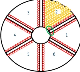
We have seen in section2.2 that performance obtained without any telescope spiders and with a continuous DM surface is very good, typically around 100nm RMS for median turbulence conditions. As the spider location and size are fixed by the telescope design there is very little we can change about their thicknesses or any other of their characteristics. M4 actuators are driven into position to a known and absolute distance from the reference body. In addition, all 6 DM segments will use a common SiC reference body and exact actuator extensions across the entire DM surface will be available. It is therefore possible to modify the behaviour of the DM by acting on the extension of the actuators. In particular, we can emulate the behaviour of a DM with a continuous surface. This is done by coupling edge actuators together in pairs as illustrated Figure 11 and Figure 12 for 2 actuators located respectively on segment 1 and segment 2. The coupling is done for all pairs of actuators directly opposite of each other. This method will naturally lead to a reduced number of degrees of freedom, but the reduction in the total fitting error is negligible [10]. On top from making it harder (but not impossible) for the DM to produce a segment piston, this method has the advantage of actually changing the data sensed by the P-WFS under the spiders and that is related to differential piston.

Figure 11: Illustration of M4 with 6 segments. The actuator locations are depicted by the coloured circles and the red circles represent the edge actuators. The coupled actuators seen Figure 12 are circled in green.

Figure 12: Illustration of the influence function created by the coupled actuators highlighted Figure 11. The gap created by the spider is clearly visible.

(10)

4 3 JO 50 300 E2 w` m 1 aNi 100 50 50

SCAO nerfermance v. seeing

Edge Coupling

f

Reference Case

i

f

50 0 0 4 0.5 0.6 0.7 0.8 0.9 1.1 1 2 Seeing [arsec]

Edae actuator coupling: 0.65 arcsec

3500 3000 2500 2 cc 2000 C 1501 1000 500 Turbulence Residual error 1000 2000 3000 4000 5000 Iteration number

4.2 Comparison to the nominal case

Figure 13 shows the SCAO performance as a function of seeing for the edge actuator coupling control strategy (red) and for the reference case (blue). For all cases, the P-WFS modulation is set to 4λ/D. The stability of the close loop is presented in terms of standard deviation and is shown to increase as the seeing degrades. We remind the reader that the median seeing condition for which the HARMONI requirements are defined is 0.65˝. The quadratic error between the reference case and the correction of the IE using EAC is reduced to 40 nm RMS for 0.65˝. Without any IE correction, the residual error is of the order of 550 nm RMS.

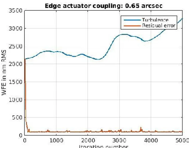
IE is created by the gap generated by the telescope spiders and the fact the differential piston is a very badly seen mode. Their appearance is triggered by residual errors in the AO correction that will create sufficient instabilities for the IE to appear. Eventually the differential piston signal will increase and the P-WFS will be able to sense it to finally bring it back to zero. For this reason, the IE will be stronger is bad seeing condition and the improvement brought by edge actuator coupling [EAC] will be more efficient for better seeing conditions. Figure 14 shows the residual error as a function of iteration time for edge actuator coupling, a P-WFS modulation of 3λ/D, and a seeing of 0.65˝. The occasional loss in performance can be clearly seen around iteration numbers 750 and 1300 for example where the performance drops slightly.

Figure 13: SCAO performance as a function of seeing. Comparison between the nominal case and the edge couple case. Modulation 4λ/D. Error bars represent the standard deviation from these results.

Figure 14: SCAO performance with edge actuator coupling as a function of loop iterations. Median seeing conditions, modulation 3λ/D.

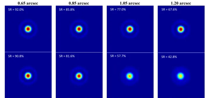
Figure 15 shows an illustration of the long-exposure PSFs for 4 different seeing conditions. The reference case shows very good correction as presented section 2.2 with residual errors of 177 nm RMS and 217 nm RMS for seeings of 1.05˝ and 1.20˝ respectively. The correction of the IE using EAC also presents good correction quality with some residual differential piston nonetheless present, especially for bad seeing conditions. The nominal seeing condition measured by ESO is 0.65 arcsec, meaning that for the vast majority of time the seeing will be below 0.85 arcsec and the correction brought by the EAC will be extremely good.

(11)

500 450 400 g350 E 300 250 W 200 M 150 100 50

SCAO performance v. modulation

-14 -f - Reference Case -f - Edge Coupling 0.65" -f - Edge Coupling 0.85" - Edge Coupling 1.05" Edge Coupling 1.20"

-0 0 2 4 6 8 10 12 Modulation [MD]

0.65 arcsec 0.85 arcsec 1.05 arcsec 1.20 arcsec

Ref er ence Co up lin g

Figure 15: Long exposure Point-Spread Function (PFS). Top: reference case. Bottom: control of the island effect (IE) using edge actuator coupling (EAC). Four seeing cases are shown. Strehl ratios are shows in the K-band. Colour LUTs are identically for a given seeing, but different between each seeing conditions.

4.3 Impact of modulation

Figure 16 presents SCAO performance as a function of P-WFS modulation both for the reference case at 0.65˝ and the EAC for varying seeing conditions. For the reference case, this shows that for a modulation of 1λ/D the performance is rather poor. As soon as the modulation is increased – between 2λ/D and 12λ/D for the range studied here - the residual error drops down to 102 nm RMS.

Figure 16: Residual error as a function of PYR modulation and seeing conditions.

Equally for the EAC case, performance changes as a function of modulation. For median seeing 0.65˝ conditions, increasing the modulation decreases performance favouring modulation of 4λ/D or below. As the turbulence is increased, the optimal modulation is also increased. In order to reach the best possible performance, it is possible to change the modulation diameter as a function of seeing. However this is likely to overcomplicate calibration/operation and forces the system to closely monitor atmospheric conditions. An alternative solution consists in keeping the modulation constant, allowing for a slight degradation in performance while keeping the AO control strategy as simple as possible. Figure 16 shows that 4λ/D is a good compromise for all seeing conditions; only rising the residual error to 110 nm RMS at 0.65˝.

SR = 92.0% SR = 85.8% SR = 67.6%

SR = 90.8% SR = 81.6%

SR = 77.0%

SR = 57.7% _{SR = 42.8%}

(12)

30 90 80 70 60 50 40 30 20 10

SCAO performance 0.65"v.NGSmagnitude

R====t,

- - Edge Coupling 0.65' - - Reference case

-6

-SR Difference

o--O`\

o-r---o-,-o

-0-8 10 12 14 16 18 GS Magnitude 600 5 50 500 rfi'a E ao0 3 Ill 300 m 2 200 50 50 50 150

SCAO nprformancp 0.65" v-tau0 dge Coupling reference Case SO deflnkion 100 -0 5 10 15 20 25 30 [ms]

4.1 Impact of NG star magnitude

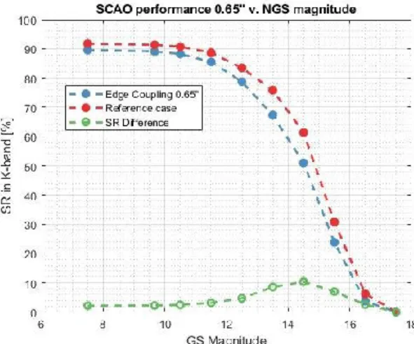
Figure 17 show the SCAO performance as a function of natural guide star magnitude for the reference case (red) and the correction of the IE using edge actuator coupling (blue). It also presents the difference in Strehl ratio between the two, with a drop in performance around 2-3% for bright stars and rising to 10% maximum at the knee of the curve when the SCAO performance starts to drop. The mean drop in performance, calculated as the difference in Strehl ratio, presented in Figure 17 is 4% throughout the NGS magnitude range studied here.

Figure 17: SCAO performance as a function of the guide star R-band magnitude.

4.2 Impact of wind

In the case of HARMONI, the final SCAO performance is limited by the DM fitting error which dominates the total error budget. That means that temporal errors shouldn’t impact performance significantly. In our case, we are in fact interested to know whether the edge actuator coupling strategy introduces any addition error on top of the performance given by the reference case. Figure 18 give the performance of the SCAO in terms of residual error as a function of atmospheric coherence time τ0 (i.e. increased wind speed in the turbulence layers). It shows clearly that there is a very limited drop in performance between the two curves (approx. an average of 10% additional error throughout). This validate the choice of edge actuator coupling to correct IE as robust for changing turbulence condition, in particular changing wind conditions.

Figure 18: Residual error as a function of τ0. The blue curve represents the edge actuator coupling, the red curve the

reference case and the orange dots reference points given by ESO’s 35-layer reference zenith profiles.

(13)

2 50

DO

50

SCAO performance 0.65" v. ACensing -f - Edge -f -Refe - - Quai Coupling ence Case Iratique Difference DO 0 600 800 1000 1200 1400 1600 1800 2000 2200 Sensing Wavelength sensing[nm] -1-OS 03

SCAO performance 0.65' v. _nsing

a-_

No Edge Coupling

102

600 800 1000 1200 1400 1600 1800 2000 2200

Sensing Wavelength Asensing [nm]

4.3 Impact of sensing wavelength

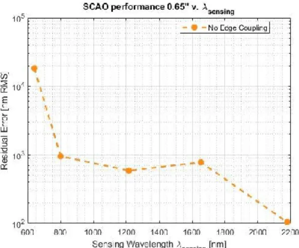
The choice of the sensing wavelength λWFS will clearly impact the AO performance, especially when the Fried parameter becomes larger than the gap between the mirror segments. The choice of λWFS for HARMONI was set during the preliminary design to be in the I-band centred on approx. 800 nm. Figure 19 presents the residual error as a function of λWFS. The modulation is set at 4λ/D for all cases, the ground-layer wind at 10 m/s (higher than the 5.5 m/s previously shown), and the seeing is 0.65 arcsec. It shows that the quadratic error between the reference case and the correction of the IE using EAC is reduced as the sensing wavelength is increased. This greatly favours the longer sensing wavelengths, as would be expected. However, when the seeing conditions degrade, the improvement brought by the edge actuator couple will also slightly degrade.

Figure 19: Residual error as a function of wavefront sensing wavelength for the reference case and the IE correction using edge actuator coupling.

Figure 20: Residual error as a function of wavefront sensing wavelength for no correction of the island effect (IE).

Figure 20 presents the residual error as a function of λWFS when no correction of the IE is performed. As in Figure 19 the correction quality improves as the sensing wavelength is increased. It is important to notice that for very long wavelengths very little error is introduced by the IE. As a matter of fact, in the K-band for 2.2 μm the quadratic error between the reference case and no IE correction is of only 18 nm and the correction appears to be stable over time. For shorter wavelengths - this is particularly the case for sensing in the H and J bands - the correction can be stable with only a few segments having an additional but constant differential piston of ±λWFS (i.e. presence of IE, but no fluctuations of the IE over time). This differential piston is stable over time, indicating that a perfect correction may still be possible by for example monitoring the shape of the PSF. For even shorter wavelengths (i.e. I-band), the correction is unstable and the differential pistons have a tendencies to slightly change over time. This can be somewhat mitigated by lowering the modulation, especially in good seeing conditions. In the R-band, the correction is unstable and large differential pistons that vary over time start to appear.

5. CONCLUSIONS

We have provided a detailed analysis in this paper a detailed analysis of the differential piston that is introduced by the adaptive optics control loop (often called the island effect). The island effect (IE) appears when the phase discontinuities in the pupil are created by large gap; these gaps are usually created by the telescope spiders. We proposed a simple solution to mitigate the island effect using edge actuator coupling. This solution consists in pairing actuators on either side of the spider 2 by 2 ensuring that they act as a single actuator with a combined and much larger influence function. We have shown that this solution performance well in the nominal case and is robust to changing conditions (turbulence, wind, natural guide star magnitude…). Edge actuator coupling is currently the baseline for correcting the island effect on HARMONI.

The perspectives of this work are to investigate ways to improve correction quality when the seeing conditions are poor, in particular by adding a penalty on the non-atmospheric differential pistons. In addition to the island effect, a currently

(14)

unknown amount of low wind effect will be present. The second step will be to investigate a correction strategy for the low wind effect and ensure it can made compatible with the IE correction.

REFERENCES

[1] Thatte, N., Clarke, F., Bryson, I., et al., "The E-ELT first light spectrograph HARMONI: capabilities and modes," Proc. of SPIE, 9908, 99081X-99081X-11 (2016)

[2] Neichel, B., Fusco, T., Sauvage, J.-F., Correia, C., et al., "The adaptive optics modes for HARMONI: from Classical to Laser Assisted Tomographic AO," Proc. of SPIE, 9909, 9909-9 (2016)

[3] Schwartz, N., Sauvage, J.F., Correia, C., Neichel, B., Blanco, L., Fusco, T., Pécontal-Rousset, A., Jarno, A., Piqueras, L., Dohlen, K. and El Hadi, K., "Preparation of AO-related observations and post-processing recipes for E-ELT HARMONI-SCAO," Proc. of SPIE, 9909, 990978-990978-10 (2016)

[4] Neichel, B., Fusco, T., Sauvage, J.-F., Correia, C., Dohlen, K., El-Hadi, K., Blanco, L., Schwartz, N., et al., "The adaptive optics modes for HARMONI: from Classical to Laser Assisted Tomographic AO," Proc. of SPIE 9909, Adaptive Optics Systems V, 990909 (2016).

[5] B. Neichel, T. Fusco, J.-F. Sauvage, C. Correia, K. Dohlen, L. Blanco, et al., "HARMONI at the diffraction limit: from single conjugate to laser tomography adaptive optics," Proc. of SPIE 10703, Adaptive Optics Systems IV (2018).

[6] Kolb, J., Gonzalez, H., Juan, C. and Tamai, R., "Relevant Atmospheric Parameters for E-ELT AO Analysis and Simulations, ESO-258292 Issue," Technical report ESO (2015).

[7] Sauvage, J.-F., Fusco, T., Lamb, M., Girard, J., et al., "Tackling down the low wind effect on SPHERE instrument," Proc. of SPIE 9909, Adaptive Optics Systems V, 990916 (2016).

[8] N’Diaye, M., Martinache, F., Jovanovic, N., Lozi, J., Guyon, O., Norris, B., Ceau, A. and Mary, D., "Calibration of the island effect: Experimental validation of closed-loop focal plane wavefront control on Subaru/SCExAO," A&A, 610, A18 (2018)

[9] Wilby, M. J., Keller, C. U., Sauvage, J. F., Fusco, T., Mouillet, D., Beuzit, J. L. and Dohlen, K, "A 'Fast and Furious' solution to the low-wind effect for SPHERE at the VLT," Proc. of SPIE 9909, Adaptive Optics Systems V, 99096C (2016).

[10] Schwartz, N., Sauvage, J.-F., Correia, C., Petit, C., Quiros-Pacheco, F., Fusco, T., Dohlen, K., El Hadi, K., Thatte, N., Clarke, F., Paufique, J., Vernet, J., "Sensing and control of segmented mirrors with a pyramid wavefront sensor in the presence of spiders," Proc. of AO4ELT5, (2016).

[11] Milli, J., Kasper, M., Mouillet, D., Sauvage, J.F., et al, "Low wind effect on VLT/SPHERE: impact, mitigation strategy with a low-emissivity coating applied to the spiders of UT3, and results," Proc. of SPIE 10703, Adaptive Optics Systems IV (2018).

[12] Esposito, S. et al., “Pyramid sensor for segmented mirror alignment,” OPTICS LETTERS, Vol. 30, No. 19, p. 2572, (2005).

[13] Verinaud, C. and Esposito, S., "Adaptive-optics correction of a stellar interferometer with a single pyramid wave-front sensor," Opt. Lett. 27, 470-472 (2002).

[14] Quirós-Pacheco, F., Conan, R., Bouchez, A., McLeod, B., "Performance of the Giant Magellan Telescope phasing system," Proc. of SPIE 9906, 99066D (2016)

[15] Bond, C.Z., Correia, C.M., Sauvage, J.F., Neichel, B. and Fusco, T., "Iterative wave-front reconstruction in the Fourier domain," Optics Express, 25(10), 11452-11465 (2017).

[16] Le Louarn, M., Béchet, C., Tallon, M., "Of Spiders and Elongated Spots," Proc. of the Third AO4ELT Conference, (2013).

[17] Bonnefond, S., Tallon, M., Le Louarn, M. and Madec, P.Y., "Wavefront reconstruction with pupil fragmentation: study of a simple case," Proc. of SPIE 9909, Adaptive Optics Systems V, 990972 (2016).

[18] Tallon, M., Le Louarn, M., "Effect of pupil fragmentation and truncation of elongated spots on wavefront reconstruction," Wavefront Sensing in the VLT/ELT era, Marseille (2016).