U
NIVERSITY OF
N
APLES
F
EDERICO
II
School of Polytechnic and Basic Sciences
Department of Chemical, Materials and Industrial Production Engineering
XXXI PhD Programme in
Industrial Products and Processes Engineering
Smart Sensor Monitoring in
Machining of Difficult-to-Cut Materials
PhD COURSE COORDINATOR
PhD CANDIDATE
Ch.mo Prof. Ing. Giuseppe Mensitieri
Ing. Francesco Napolitano
PhD SUPERVISOR
Ch.mo Prof. Ing. Roberto Teti
PhD CO-SUPERVISOR
Dr. Ing. Alessandra Caggiano
Index
Index
LIST OF FIGURES ... III
LIST OF TABLES ... VI
1. INTRODUCTION ... 1
2. SENSOR MONITORING OF MACHINING PROCESSES ... 3
2.1SENSOR MONITORING APPLICATIONS ... 3
2.1.1 Tool conditions ... 3
2.1.2 Surface integrity ... 4
2.1.3 Process conditions ... 4
2.1.4 Chip form ... 5
2.1.5 Machine tool state ... 5
2.1.6 Other applications ... 6
2.2SENSORS FOR MACHINING PROCESS MONITORING ... 6
2.2.1 Motor Power and Current ... 6
2.2.2 Force and torque ... 7
2.2.3 Acoustic emission ... 8
2.2.4 Vibration ... 8
2.2.5 Other sensors ... 9
2.3ADVANCED SENSOR SIGNAL PROCESSING METHODS ... 9
2.3.1 Signal conditioning and pre-processing ... 10
2.3.2 Signal feature extraction ... 11
2.3.2.1 Time domain ... 11
2.3.2.2 Frequency domain ... 11
2.3.3 Signal feature selection ... 12
2.4DECISION MAKING SYSTEMS ... 13
2.4.1 Neural networks ... 15
2.4.2 Fuzzy logic ... 16
2.4.3 Other decision making systems ... 17
2.5SENSOR FUSION TECHNOLOGY ... 18
2.6CLOUD MANUFACTURING FOR MACHINING PROCESS MONITORING ... 19
2.7RESEARCH GAP ... 20
2.7.1 Gap identification ... 20
2.7.2 Objectives ... 21
3. SMART SENSOR MONITORING OF TITANIUM ALLOY DRY TURNING
... 22
3.1THE FRAMEWORK ... 22
3.1.1 CAPRI project on “Landing Gear with Intelligent Actuation” ... 23
3.2EXPERIMENTAL TESTING CAMPAIGN ... 23
3.2.1 Multiple sensor system setup ... 24
Index
3.2.3 Cutting tool specifications and process parameters ... 33
3.3TOOL WEAR MEASUREMENT AND WEAR CURVE CONSTRUCTION ... 34
3.4SIGNAL PROCESSING AND FEATURE EXTRACTION ... 37
3.4.1 Signal segmentation and resampling ... 39
3.4.2 Signal feature extraction ... 41
3.4.3 Signal feature selection ... 42
3.5TOOL WEAR CURVE RECONSTRUCTION AND GENERATION THROUGH INTELLIGENT METHODS ... 43
3.5.1 Tool wear curve reconstruction ... 43
3.5.2 Tool wear curve generation... 44
3.6RESULTS AND DISCUSSION ... 46
4. SMART SENSOR MONITORING OF CFRP/CFRP AND AL/CFRP STACK
DRILLING ... 48
4.1THE FRAMEWORK ... 48
4.1.1 Applications ... 50
4.2EXPERIMENTAL TESTING CAMPAIGN ... 51
4.2.1 Multiple sensor system setup ... 51
4.2.2 Workpiece material ... 54
4.2.3 Cutting tool specifications and process parameters ... 57
4.3TOOL WEAR MEASUREMENT AND WEAR CURVE CONSTRUCTION ... 58
4.4SIGNAL PROCESSING AND FEATURE EXTRACTION ... 64
4.4.1 Signal segmentation ... 65
4.4.2 Signal features extraction ... 68
4.4.2.1 Time domain features ... 69
4.4.2.2 Frequency domain features ... 71
4.4.3 Signal features selection ... 76
4.4.3.1 Feature dimensionality reduction ... 77
4.5TOOL WEAR CURVE RECONSTRUCTION THROUGH INTELLIGENT METHODS ... 79
4.6RESULTS AND DISCUSSION ... 81
4.6.1 Tool wear forecast in drilling ... 81
4.6.2 Feature dimensionality reduction ... 84
5. SUMMARY AND FUTURE DEVELOPMENTS ... 86
5.1CLOUD MANUFACTURING APPROACH ... 87
List of Figures
List of Figures
Figure 1. Spindle motor with integrated sensor ring (G. Byrne and O’ Donnell 2007) ... 7
Figure 2. Advanced signal processing procedure (Teti et al. 2010) ... 10
Figure 3. Frequency of usage of AI approaches in intelligent machining systems according to the references found in the research platform ISI-Web of knowledge from 2002 to 2007 (Abellan-Nebot and Romero Subirón 2010). ... 14
Figure 4. Fuzzy inference system implementation steps (Teti et al. 2010). ... 17
Figure 5. Doosan PUMA400LM CNC lathe. ... 24
Figure 6. Multiple sensor system mounted on the tool holder (Alessandra Caggiano, Napolitano, and Teti 2017). ... 25
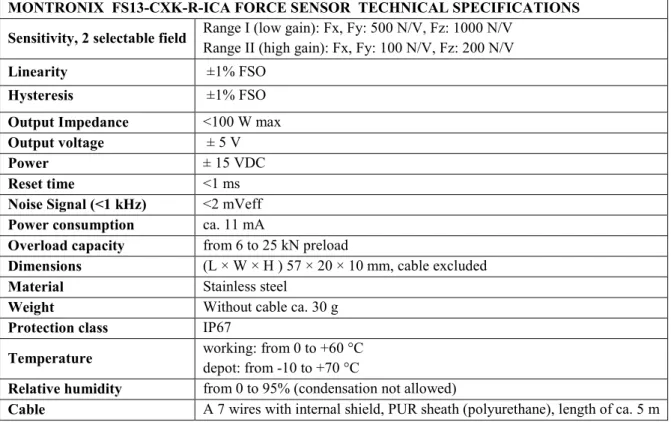
Figure 7. 3D Force sensor Montronix FS13-CXK-R-ICA. ... 25
Figure 8. Set-up of the Montronix TSFA3-ICA 3D force sensor amplifier. ... 26
Figure 9. Acoustic emission sensor Montronix BV-100. ... 27
Figure 10. Acoustic Emission sensor amplifier Montronix TSVA2-DGM-BV. ... 28
Figure 11. Vibration sensor Montronix Spectra TM Pulse. ... 29
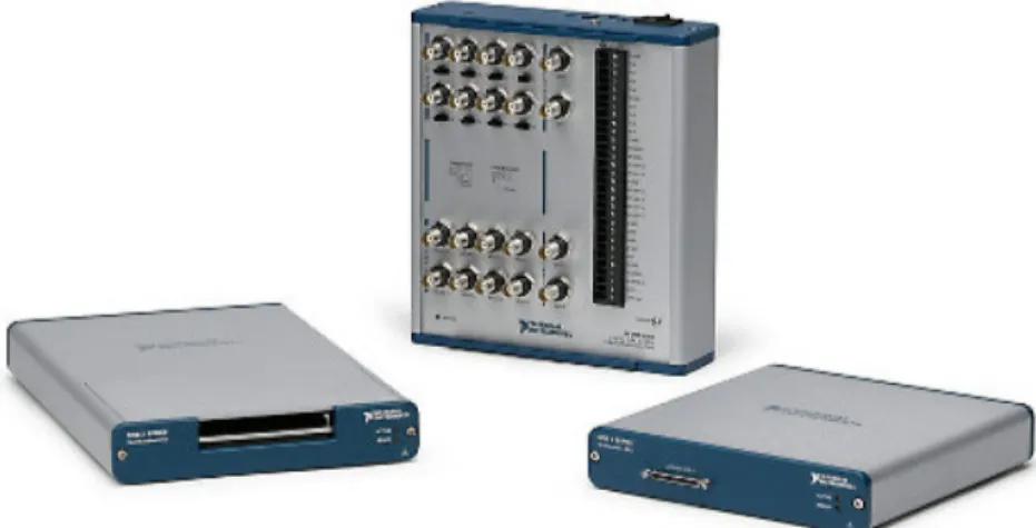
Figure 12. National Instrument NI USB-6361 digitizing board. ... 31
Figure 13. Cutting insert CNMG120404-MS MT9015. ... 33
Figure 14. Wear zone of the cutting edge(ISO 3685:1993). ... 34
Figure 15. Tool wear measurement on the acquired image. ... 35
Figure 16. Dino Lite Microscope. ... 35
Figure 17. Dino Lite Microscope mounted on its magnetic support. ... 36
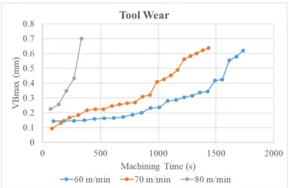
Figure 18. Measured tool flank wear values vs machining time for v1 = 60 m/min, v2 = 70 m/min, v3 = 80 m/min (f = 0.2 mm/rev, d = 0.5mm). ... 36
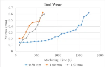
Figure 19. Measured tool flank wear values vs machining time for d1 = 0.5 mm, d2 = 1 mm, d3 = 1.5 mm (v = 60 m/min, f = 0.2 mm/rev). ... 37
Figure 20. Measured tool flank wear values vs machining time for f1 = 0.2 mm/rev, f2 = 0.25 mm/rev, f3 = 0.3 mm/rev (v = 60 m/min, d = 0.5 mm). ... 37
Figure 21. Acquired Force signals. ... 38
Figure 22. Acquired Acoustic Emission RMS and Vibration Acceleration signals. ... 38
Figure 23. Acquired Acceleration signals. ... 39
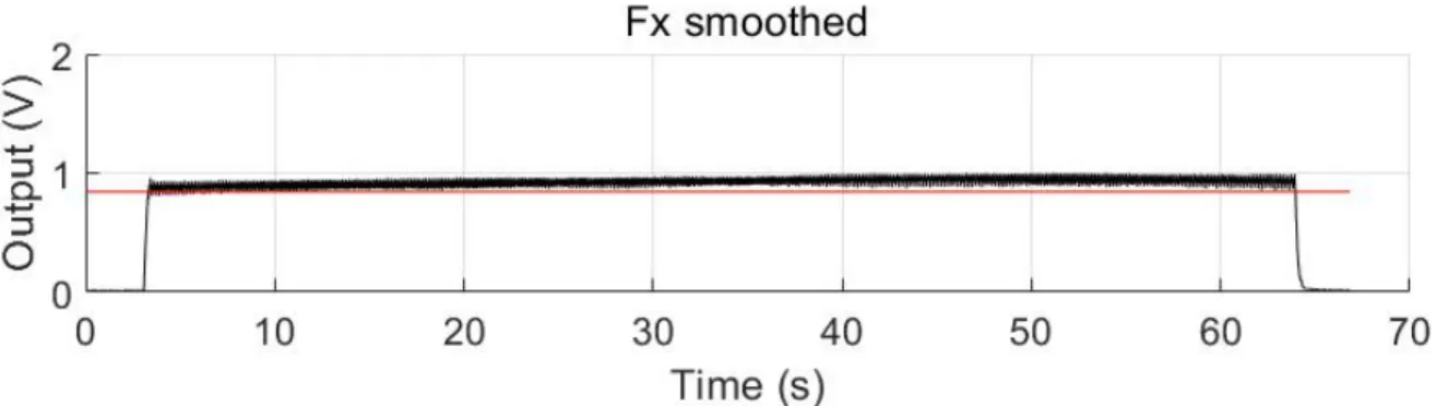
Figure 24. Moving average of Fx cutting force component signal and set threshold (red line). ... 39
Figure 25. Segmented Fx, Fy, Fz cutting force components signals. ... 40
Figure 26. Segmented acoustic emission RMS and vibration acceleration RMS signals. ... 40
Figure 27. Segmented Ax, Ay and Az vibration acceleration signals... 41
Figure 28. Extracted statistical sensor signal features in time domain. ... 42
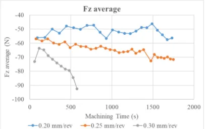
Figure 29. Average of Fz cutting force component signal, Fzav, vs machining time for f1 = 0.2 mm/rev, f2 = 0.25 mm/rev, f3 = 0.3 mm/rev (v = 60 m/min, d = 0.5 mm). ... 43
Figure 30. Artificial Neural Network architecture. ... 43
Figure 31. ANN output vs measured VBmax for turning test at v = 60 m/min, f = 0.25 mm/rev, d = 0.5 mm. ANN configuration: 9-18-1. MSE = 0.000639. ... 46
List of Figures
Figure 32. ANN entire tool wear curve generation. The tool wear curve for v1 = 60 m/min, f1 = 0.25 mm/rev, d1 = 1.5 mm is obtained using a training set comprising sensor signal
features and corresponding tool wear values for v2 = 60 m/min, f2 = 0.20 mm/rev, d2 = 1.5 mm and v3 = 60 m/min, f3 = 0.30 mm/rev, d3 = 1.5 mm. ANN configuration: 12-24-1. MSE =
0.01373. ... 47
Figure 33. Drilling basic motions. ... 49
Figure 34. Multiple sensors system for drilling process monitoring setup. ... 52
Figure 35. (a) Kistler 9257 piezoelectric dynamometer; (b) Kistler 9277A25 piezoelectric dynamometer. ... 53
Figure 36. Kistler 5007 amplifiers. ... 53
Figure 37. Acoustic Emission and Vibration Acceleration amplifier settings. ... 54
Figure 38. (a) Vacuum bag moulding; (b) Autoclave. ... 55
Figure 39. Laminates profiles and their surface textures. ... 56
Figure 40. Standard geometry of a twist drill (Mikell P. Groover 2014). ... 57
Figure 41. (a) Innovative step drill bit. (b) Traditional twist drill bit. ... 58
Figure 42. Schematic representation of twist drill (Stephenson and Agapiou 2006). ... 59
Figure 43. Tool wear as a function of cutting time (Marinov 2004). ... 60
Figure 44. Effect of cutting speed on tool wear and tool life for three cutting speeds. ... 60
Figure 45. (a) Tesa Visio V-200 optical microscope, (b) clamping system. ... 61
Figure 46. VB max and VB tool wear measurement on innovative drill bit... 61
Figure 47. VB max and VB tool wear measurement on traditional drill bit. ... 62
Figure 48. Tool wear measurement scheme for drill bits (Dolinšek, Šuštaršič, and Kopač 2001). ... 62
Figure 49. Tool wear values and interpolated curves. Traditional drill bits. ... 63
Figure 50. Tool wear values and interpolated curves. Innovative drill bits. ... 63
Figure 51. Acquired Thrust Force signal. ... 64
Figure 52. Acquired Torque signal. ... 64
Figure 53. Acquired Acoustic emission RMS signal. ... 65
Figure 54. Acquired Vibration Acceleration signal. ... 65
Figure 55. Filtered Thrust Force signal. ... 66
Figure 56. Start point and end point on the acquired Thrust Force signal. ... 66
Figure 57. Segmented Thrust Force signal. ... 67
Figure 58. Segmented Torque signal. ... 67
Figure 59. Segmented Acoustic Emission RMS signal. ... 68
Figure 60. Segmented Vibration Acceleration RMS signal. ... 68
Figure 61. Sensor signal extracted features in the case study A. ... 69
Figure 62. Sensor signal extracted features in the case study C. ... 69
Figure 63. Thrust Force Average for traditional twist drill bit d = 4.85 mm. ... 70
Figure 64. Thrust Force Variance for traditional twist drill bit d = 4.85 mm. ... 70
Figure 65. Thrust Force Skewness for traditional twist drill bit d = 4.85 mm. ... 71
Figure 66. Thrust Force Kurtosis for traditional twist drill bit d = 4.85 mm. ... 71
Figure 67. Fibre cutting angle variations during CFRP drilling. ... 72
List of Figures
Figure 69. Single-Sided Amplitude Spectrum of the Thrust Force signals acquired in drilling tests at 3000 rpm, 0.15 mm/rev. ... 73 Figure 70. Evolution of peaks detected in frequency domain using discrete Fourier Transform ... 73 Figure 71. Segmented and filtered thrust force signal with separation line for Aluminium drilling portion and CFRP drilling portion. ... 74 Figure 72. Sensor signal extracted features in the case study B. ... 75 Figure 73. Scree plot reporting the variance explained as a function of the principal
components for all the drilling tests. ... 78 Figure 74. Scores of the first principal component, PC1, and measured tool wear values, VB, vs hole no. for test T3 (v = 6000 rpm, f = 0.15 mm/rev). ... 79 Figure 75. ANN architecture proposed in the case study A. ... 80 Figure 76. ANN architecture proposed in the case study C. ... 81 Figure 77. RMSE prediction performance of the ANN trained with diverse numbers, m, of SFPVs for the tests with traditional drill bits. ... 81 Figure 78. RMSE prediction performance of the ANN trained with diverse numbers, m, of SFPVs for the tests with innovative drill bits. ... 82 Figure 79. Worst case ANN forecast: experimental tests at 2700 rpm – 0.11 mm/rev with innovative drill bit. ... 83 Figure 80. Best case ANN forecast: experimental tests at 6000 rpm – 0.20 mm/rev with innovative drill bit. ... 83 Figure 81. Regression plot between ANN predicted and measured VB for test v = 6000 rpm, f = 0.15 mm/rev. ANN configuration: 3-3-1. RMSE = 4.09E-04. ... 85
List of Tables
List of Tables
Table 1. Comparison between main properties of Ti6Al4V and steel (Donachie 1983). ... 22
Table 2. Characteristics of the force sensor (Teti et al. 2006). ... 26
Table 3. Technical characteristic of 3D force sensor amplifier. ... 27
Table 4. Technical specifications of Acoustic Emission sensor Montronix BV-100. ... 28
Table 5. Technical specifications of AE amplifier Montronix TSVA2-DGM-BV. ... 29
Table 6.Technical specifications of transmission unit. ... 30
Table 7.Technical specifications of Spectra Pulse Vibration Sensor. ... 31
Table 8. Technical characteristic of digitizing board NI USB-6361. ... 32
Table 9. Cutting conditions employed in the experimental campaign. ... 33
Table 10. Verification of correlations based on Pearson correlation coefficient. ... 45
Table 11. Overall Mean Square Error (MSE) obtained by ANN tool wear reconstruction for all the turning tests carried out at v = 60 m/min. ... 46
Table 12. Summary of the experimental setup for drilling case studies. ... 51
Table 13. Chemical composition of the Aluminium 2024 alloy. ... 56
Table 14. Physical, mechanical and thermal properties of the Aluminium 2024 alloy. ... 57
Table 15. Experimental testing conditions for case studies A and C. ... 58
Table 16. Experimental testing conditions for case study B. ... 58
Table 17. List of most correlated features (case study B). ... 77
Table 18. Overall Root Mean Square Error (RMSE) obtained by ANN tool wear estimation for all the drilling tests. ... 84
1. Introduction
1. Introduction
The research activities presented in this thesis are focused on the development of smart sensor monitoring procedures applied to diverse machining processes with particular reference to the machining of difficult-to-cut materials. This work will describe the whole smart sensor monitoring procedure starting from the configuration of the multiple sensor monitoring system for each specific application and proceeding with the methodologies for sensor signal detection and analysis aimed at the extraction of signal features to feed to intelligent decision-making systems based on artificial neural networks. The final aim is to perform tool condition monitoring in advanced machining processes in terms of tool wear diagnosis and forecast, in the perspective of zero defect manufacturing and green technologies.
The work has been addressed within the framework of the national MIUR PON research project CAPRI, acronym for “Carrello per atterraggio con attuazione intelligente” (Landing Gear with Intelligent Actuation), and the research project STEP FAR, acronym for “Sviluppo di materiali e Tecnologie Ecocompatibili, di Processi di Foratura, taglio e di Assemblaggio Robotizzato” (Development of eco-compatible materials and technologies for robotised drilling and assembly processes). Both projects are sponsored by DAC, the Campania Technological Aerospace District, and involve two aerospace industries, Magnaghi Aeronautica S.p.A. and Leonardo S.p.A., respectively. Due to the industrial framework in which the projects were developed and taking advantage of the support from the industrial partners, the project activities have been carried out with the aim to contribute to the scientific research in the field of machining process monitoring as well as to promote the industrial applicability of the results.
The thesis was structured in order to illustrate all the methodologies, the experimental tests and the results obtained from the research activities. It begins with an introduction to “Sensor monitoring of machining processes” (Chapter 2) with particular attention to the main sensor monitoring applications and the types of sensors which are employed in machining. The key methods for advanced sensor signal processing, including the implementation of sensor fusion technology, are discussed in details as they represent the basic input for cognitive decision-making systems construction. The chapter finally presents a brief discussion on cloud-based manufacturing which will represent one of the future developments of this research work.
Chapters 3 and 4 illustrate the case studies of machining process sensor monitoring investigated in the research work. Within the CAPRI project, the feasibility of the dry turning process of Ti6Al4V alloy (Chapter 3) was studied with particular attention to the optimization of the machining parameters avoiding the use of coolant fluids. Since very rapid tool wear is experienced during dry machining of Titanium alloys, the multiple sensor monitoring system was used in order to develop a methodology based on a smart system for on line tool wear detection in terms of maximum flank wear land. Within the STEP FAR project, the drilling process of carbon fibre reinforced (CFRP) composite materials was studied using diverse experimental set-ups. Regarding the tools, three different types of drill bit were employed, including traditional as well as innovative geometry ones. Concerning the investigated materials, two different types of stack configurations were employed, namely CFRP/CFRP stacks and hybrid Al/CFRP stacks. Consequently, the machining parameters for each experimental campaign were varied, and also the methods for signal analysis were changed to verify the performance of the different methodologies. Finally, for each case different neural network configurations were investigated for cognitive-based decision making. First of all, the applicability of the system was tested in order to perform tool wear diagnosis and forecast. Then, the discussion proceeds with a further aim of the research work, which is the reduction of the number of selected sensor signal features, in order to improve the performance of the cognitive decision-making system, simplify modelling and facilitate the implementation of these methodologies in a cloud manufacturing approach to tool condition monitoring.
Sensor fusion methodologies were applied to the extracted and selected sensor signal features in the perspective of feature reduction with the purpose to implement these procedures for big data
1. Introduction
condition monitoring methodologies based on multiple sensor signal acquisition and processing is illustrated, with particular reference to the reliable assessment of tool state in order to avoid too early or too late cutting tool substitution that negatively affect machining time and cost.
2. Sensor monitoring of machining processes
2. Sensor monitoring of machining
processes
In the last years many studies showed that the availability of real-time data regarding the process operating conditions is the base of the success of modern flexible manufacturing systems. Due to the difficulties to find reliable models of production systems performance prediction it is necessary to assemble improved multiple sensors systems and to develop more sophisticated techniques for processing the sensor data output, in order to increase the efficiency of the actual monitoring systems employed for process monitoring and control of production.
Several authors of recent research studies have shown the effectiveness of sensor monitoring techniques based on the signal analysis (Teti et al. 2010). The aim of sensor monitoring is to increase the machining information reliability in order to make proper diagnosis about the status of the process through the selection of the appropriate features.
2.1 Sensor Monitoring Applications
Advanced monitoring of machining operations may have several objectives such as tool condition monitoring (TCM), surface integrity, process conditions monitoring, chip form classification and monitoring of the machine tool state (Teti et al. 2010).
2.1.1 Tool conditions
The following list summarizes some of the most important and notable applications in tool condition monitoring:
Analysis of acoustic emission (AE) using the wavelet packet decomposition method (WPD) for automatic classification of tool wear in milling (S. Wu et al. 2014).
Development of correlations in broaching between tool conditions and output signals of multiple sensors, i.e. AE, vibration, cutting force, hydraulic pressure and spindle power of the broaching machine, mounted on the machine tool (Dragos A Axinte and Gindy 2003). The spindle power signal was used for tool condition monitoring in milling, drilling and turning, it turned out to be successful in continuous turning and drilling but not efficient in discontinuous milling.
Application to identify real-time tool breakage in milling operations based on the analysis of indirect measurements of cutting force through feed drive AC motor current (JM Lee et al. 1995).
Development of a laser displacement meter for online tool geometry (Ryabov, Mori, and Kasashima 1996).
Development of an online tool condition monitoring system based on vibrations and cutting forces monitoring (D. Dimla and Lister 2000).
Online estimation of drill wear during drilling operations based on spindle motor power signal (H. Y. Kim et al. 2002).
Use of micro-scale thermal imaging to identify effects of steel machinability on cutting zone temperature and related tool wear mechanisms (Arrazola et al. 2008).
Analysis and comparison of cost effective methods for tool breakage detection by performing trials on ultra-precision micro-milling machine (Gandarias et al. 2006).
2. Sensor monitoring of machining processes
2.1.2 Surface integrity
Concerning monitoring and control of surface integrity in manufacturing processes, a number of applications and studies have been developed. The most remarkable are illustrated below:
Online estimation of surface roughness (Ra) and dimensional deviation (DD) in turning using neural network. Cutting feed, depth of cut and two components of the cutting force (the feed and radial force components) appears to be the most significant features to be monitored (Azouzi and Guillot 1997).
Correlation of surface and cutting force in end milling processes based on a statistical approach (Huang and Chen 2003).
Prediction of surface roughness in turning based on cutting vibration parameters and FFT analysis (Abouelatta and Màdl 2001).
Decomposition of the vibration signals for in-process prediction of surface roughness in turning based on singular spectrum analysis (Salgado et al. 2009).
Real-time surface roughness prediction and machining trouble during cutting operation through time series analysis of vibration acceleration signals measured (Song et al. 2005).
Assessment of machined surface quality after broaching, in terms of geometrical accuracy, burr formation, chatter marks and surface anomalies, based on the monitoring of multiple sensors signals, i.e. acoustic emission, vibration and cutting force. Cutting force in broaching proved to be efficient in detecting of small surface anomalies (Dragos Axinte et al. 2004).
Development of a real-time monitoring system in hard machining to correlate AE parameters and white layer, surface finish and tool wear. The results showed that AERMS, frequency and count rate seems to be correlated with white layer formation and therefore suitable to monitor surface integrity factors (Guo and Ammula 2005).
Recognition of grinding burns in cylindrical plunge grinding processes through AE signal analysis (Kwak and Song 2001).
Real-time surface roughness prediction method based on a simple linear regression model using the displacement signal of spindle motion (Chang et al. 2007).
Process monitoring in abusive broaching and milling of difficult-to-machine aerospace materials for surface anomalies detection based on AE signals and cutting force data (D Axinte et al. 2005; Marinescu and Axinte 2009).
Analysis of the dynamics of broaching of complex part features. Inclined chatter surface marks, because of cutting edges specific geometry were linked through force and acceleration signal analysis revealed (D A Axinte 2007).
Detection of workpiece surface discontinuities during multiple cutting edge machining through an array of three AE sensors (A. Axinte, Natarajan, and Gindy 2005; Marinescu and Axinte 2008).
Determination of the cutting speed and feed rate effect on the quality of drilled holes in carbon fibre composites through cutting forces and temperature analysis (Rawat and Attia 2009).
2.1.3 Process conditions
The monitoring of process conditions represents another relevant aspect concerning the machining process analysis. Below are reported important applications and developments:
Classification of drilling operations in normal and abnormal, e.g. tool breakage or missing tool, based on spindle power signals (Brophy, Kelly, and Byrne 2002).
Fault detection method in tapping under different fault conditions based on torque and radial force (Mezentsev et al. 2002).
2. Sensor monitoring of machining processes
Development of an online machining monitoring system for machining operations of aero engine materials experimentally validated on PXI and LabVIEW platforms (Shy, Axinte, and Gindy 2007).
Development of a process monitoring system in Al alloy milling based on sound energy sensors, frequency analysis and cognitive processing of audible sound signal features to identify variable process conditions (Rubio and Teti 2009).
Implementation of a generalised internet-based process monitoring facility for process optimisation and simulation forming a Remote Machine Monitoring System (RMMS) (Chen et al. 2002).
Development of an online polishing expert system based on AE signals integrated with a multiple sensor system which can detect in real time polishing status and subsequently adjust the polishing parameters initially set (Ahn et al. 2001).
Assessment of cutting variables, such as shear angle, chip thickness, tool vibration amplitude, strain, strain rate, and chip type in orthogonal turning tests using high speed photography combined with laser printed square grid (Pujana, Arrazola, and Villar 2008).
Development of an innovative non-stationary process condition monitoring method based on time-frequency distribution analysis and a singular value decomposition approach (Gu, Ni, and Yuan 2002).
2.1.4 Chip form
As regards the applications developed for chip conditions, the following papers illustrates effective applications:
Filtered AE spectrum employ components for chip form classification (Govekar, Gradisek, and Grabec 2000).
Monitoring method based on neural network and spindle motor power to detect the state of chip disposal in drilling (H. Y. Kim et al. 2002).
Chip form recognition based on wavelet packet transform (WPT) and spectral estimation of cutting force signals (Teti et al. 2006).
Chip form characterization (chip entanglements, chip size, and chip shape) under different dry cutting conditions using geometric transformations of the control variables (Venuvinod and Djordjevich 1996).
Development and testing of a system for the automatic chip breaking detection using frequency analysis of cutting forces (Andreasen and De Chiffre 1998).
2.1.5 Machine tool state
Finally, as far as machine tool state monitoring, the main applications studied and developed are the followings:
Detection and comparison between characteristic parameters of signals available in controlled drives (position, speed and motor current) and the current ones (Verl et al. 2009).
Design and implementation of an integrated intelligent monitoring system, with modular and reconfigurable structure. This system monitors a total of 72 diagnostic features (power, vibration, temperature and pressure of the drives and spindles) (Zhou et al. 2000).
Condition monitoring technique based on vibration, acoustic emission, Shock Pulse Method (SPM) and surface roughness for fault detection of critical subsystems identified by a failure frequency analysis (Saravanan, Yadava, and Rao 2006).
2. Sensor monitoring of machining processes
2.1.6 Other applications
The sensor monitoring could be also used for other objectives. One of these further applications is the monitoring of energy consumption, especially in the green technology perspective several models were developed in order to evaluate the energy efficiency through the monitoring of energy consumption with the aim to avoid excessive waste of energy resources (Herrmann and Thiede 2009; Hu et al. 2012; Diaz et al. 2009; Vijayaraghavan and Dornfeld 2010).
Another application of the sensor monitoring systems concerns the machine maintenance. One study is focused on the implementation of monitoring system in order to perform a proactive maintenance instead of the traditional reactive sensor-based maintenance (Jay Lee 1995). Moreover, a review of methods and systems for diagnostic and prognostic of mechanical systems through condition-based maintenance paradigm allows to compare the different models, algorithms and technologies for data processing and maintenance decision-making (Jardine, Lin, and Banjevic 2006).
2.2 Sensors for machining process monitoring
The optimization of the machining process performance is the purpose of the application of sensors in machining processes to continuously monitor the manufacturing operations. This monitoring is done through diverse measuring techniques that can be distinguished as direct and indirect approaches.
Referring the techniques to the measurement of the actual quantity of a given variable, e.g. tool wear, is has the direct techniques. Other examples of direct measurement techniques applicable to monitoring of machining processes are the use of cameras for visual inspection, radioactive isotopes, laser beams, and electrical resistance. These type of technique may be limited by the access problems during machining, illumination and the use of cutting fluid so they remain confined only to laboratory environments. However, the direct measurement techniques are highly accurate and for this reason are extensively employed in research laboratories to monitor fundamental measurable variables during the machining processes.
Concerning the indirect measurement techniques, the actual quantity of a measured variable is correlated to an auxiliary quantity through an existing correlation. For this reason they are less accurate compared to direct method but give the advantage of being less complex to apply in the machining process and more appropriate to use in the industrial environments.
2.2.1 Motor Power and Current
Electric drives and spindles provide the mechanical force for material removal from the workpiece. The measurement of motor power or current or other motor related parameters can give some information about process and tool conditions. It is important that the embedded devices employed to monitor the motor related parameter do not influence negatively the machining process, it is possible to measure power through the drive control loop, particularly interesting in production environment (G. Byrne et al. 1995).
A cheap and economical monitoring solution in machining operations is retrofit power measurements. Nowadays the direct access to motor power and motor current signals using numerical controller is ensured by the most recent control systems (Oliveira et al. 2008). Recently there is the development of software integrated in the CNC control with the aim to improve the use of Human Machine Interface (HMI). The internal control signals and the additional sensors, now implemented in the machines, are based on the extension of Adaptive Control Optimise (ACO) and Adaptive Control Constraint (ACC) algorithms (Klocke, Wirtz, and Veselovac 2009). Power
2. Sensor monitoring of machining processes
measurement is already enabled in the drive controller and is adequate for use in the machining environments (G. Byrne et al. 1995). The power measurement technology leads to the application of another technique in order to demonstrate high quality signal information for process condition monitoring (Pritschow and Kramer 2005)
2.2.2 Force and torque
The mechanical machining processes require the application of mechanical forces in order to separate and remove the material from the raw workpiece. So the monitoring of cutting forces is essential for the process condition identification, cutting tool failure detection and workpiece quality assessment (G. I. Byrne, Dornfeld, and Denkena 2003). Similarly to the cutting force, also the measurement of the torsional applied load, measured by torque sensors, could be useful for the process characterization. Even though the measurement technology is the same, the application and the method of signal transmission of torque and force sensors are quite different. Force and torque sensors are generally used to measure the deformation of an elastic element and convert it into the applied force element or torsional load. The types of sensors employed for these acquisitions can be divided into two basic groups: piezoelectric and strain based sensors.
For direct force measurement, piezoelectric sensors should be mounted in line with the force path, multicomponent force transducers are employed where flexibility requirements exist such as experimental laboratory environments. Other types include rotating cutting force dynamometers that are able to acquire torque and the three components of the force. These devices have been used in monitoring of high speed milling where the speed is up to 20,000 rpm. Nowadays the integration of force and torque sensors in the CNC structure is increasing especially in drilling (G. Byrne and O’ Donnell 2007) and milling (Qiao and Zhu 2012) machine tools. Figure 1 shows an integrated force sensor ring in the motor spindle, for the integration is required the isolation of the process phenomena from spindle and machine dynamics (Jun et al. 2002; Korkut 2003).
Figure 1. Spindle motor with integrated sensor ring (G. Byrne and O’ Donnell 2007)
The strain gauges are considered stable and offer reasonably high frequency response, they are force sensors which deform when a force is applied. An application for the acquisition of static and dynamic forces is developed by combining strain gauges and piezoelectric sensor into a single instrument (J. Kim and Kim 1997). Another application provides the detection and measurement of the three cutting components of the force during milling, this is ensured by the development of a
2. Sensor monitoring of machining processes
strain based force sensor (Korkut 2003). Also on the development of a strain based sensor is based another application in which this sensor is placed between the cutting tool and the tool holder for conventional milling monitoring (Smith, Smith, and Tlusty 1998).
2.2.3 Acoustic emission
The acoustic emission (AE) is also measured and acquired during the machining processes, in order to do this measurement the piezoelectric sensor is one of the most adequate technology (Rogers 1979). Wide bandwidth is required in order to detect a big part of the phenomena in machining (100 to 900 kHz), it could be also used as root mean square (RMS) signal in order to reduce the dimension of the data to manage (X. Li 2002).
The principles to detect and monitor AE signals are based on capacitance or piezoelectric. In the first case the capacitance in the sensor changes as the distance between two parallel plate changes. This technique is considered highly accurate especially for the calibration of other AE sensors but these sensors are highly sensitive and are highly affected by position and mounting so they are inadequate in monitoring machining processes where the operating environment is harsh (Hundt et al. 1994). In the second case the piezoelectric thin film sensor is placed between the cutting insert and the tool holder, this makes the sensor more sensitive to changes due to the fact that is very closely located to the cutting process and it is also characterized by a very large frequency bandwidth.
The use of fibre optics allows to develop alternative and innovative approach (Carolan et al. 1997a, 1997b), the main advantage of this method is constituted by the fact that is a no contact method and it allows the transmission of the signal between the source and the sensor, this technology has other several strengths such as flat frequency, absolute calibration and the broader bandwidth compared to the other conventional methods. However the piezoelectric thin film sensor and fibre optics based AE sensor types have been extensively employed in laboratory environments but not yet in industrial contexts.
Regarding the AE signals, they are characterized by high frequency and low amplitude and this makes these signals suitable for transmission through a coupling fluid. As a matter of fact if the sensor is placed on the coolant supply nozzle, the coolant represents the transmission mechanism (Inasaki 1998). This application is also used with a nonintrusive coupling fluid to link the AE sensor to the spindle drive shaft (Hutton and Hu 1999; X. Li, Dong, and Yuan 1999). The method of coupling fluid is suitable in milling, drilling and other machining processes with rotating cutting tools.
It reports slip rings, inductive coupling and radio frequency transmission between the other available techniques for signal transmission and coupling between the AE sensor and the AE signal processor (Karpuschewski, Wehmeier, and Inasaki 2000; Inasaki 1998). Another research study proposed that the AE signal should be continuously reflected by the inner surfaces of the structure where the AE sensor is mounted (Krzysztof Jemielniak 2001).
2.2.4 Vibration
In the wide variety of devices to detect vibrations, the piezoelectric transduction is the most commonly employed in the machining operations. The vibrations generated during metal cutting can be considered dependent or independent from the cutting process. For example the vibration generated by other machines or by machine components are considered independent from the machining process. Instead the interrupted cutting can be considered as vibrations derived from metal cutting. As mentioned before the conditions of the cutting tool determine the aspect of the signals acquired so they have a significant impact also on the vibrations produced; chatter, which
2. Sensor monitoring of machining processes
is defined as self-excited vibration, is one of the common known types of vibration in machining, it is very destructive and negatively affects surface finish and tool life.
2.2.5 Other sensors
Beyond the most employed sensors in the machining process monitoring there are several other types which have been studied and used by the researchers in the same field of applications:
micro sensors for temperature measurements in the cutting tool insert (Biermann et al. 2013; Yang et al. 2014).
Other devices for temperature monitoring and measurement (Davies et al. 2007)
Vision systems for tool condition monitoring based on temperature measurement (Kurada and Bradley 1997; Pittalà and Monno 2011)
Lasers for cutting edge profile measuring of cutting tool in milling (Ryabov, Mori, and Kasashima 1996).
Strain and temperature sensors (Shinno and Hashizume 1997). Sound and image analysis (Mannan, Kassim, and Jing 2000). Ultrasound techniques (Abu-zahra and Yu 2000).
Laser light with reflected light intensity measurement (Wong et al. 1997).
Bifurcated optic fibre with reflected light intensity measurement (Choudhury, Jain, and Rama Rao 1999).
2.3 Advanced sensor signal processing methods
The sensor signals properly acquired can be used to extract a proper number of sensor signal features (SFs) which are indicative of the machining process state. The features extracted can be correlated to the monitoring output, e.g. tool wear and process conditions (D. S. Dimla 2000; Sick 2002; X. Li 2002).
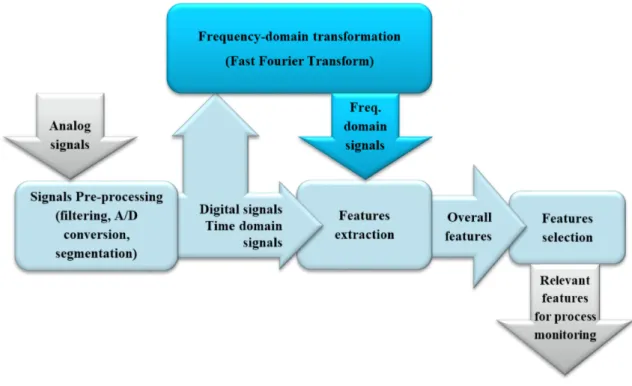
In Figure 2 is illustrated the sequence of the actions which can be done in order to apply the advanced signal processing methodology. In the first stage there are the signal pre-processing operations (filtering, amplification, A/D conversion, and segmentation), if it is necessary in this stage the signal transformation into frequency or time-frequency domain happens (Fourier Transform, wavelet transform, etc.). In the next stage the features are extracted and in the last stage the features selection takes place because there are many diverse descriptors from different sensor signals so it is important to identify the most relevant for process description. Finally they will be integrated into the tool or process condition diagnosis system.
2. Sensor monitoring of machining processes
Figure 2. Advanced signal processing procedure (Teti et al. 2010)
2.3.1 Signal conditioning and pre-processing
Analogue signals require pre-processing operations in order to be converted into digital signals. The conditioning procedure is applied at each sensor (e.g. charge amplifier, piezotron coupler, etc.). The piezoelectric AE sensor, the dynamometers and the accelerometers which are located close to the cutting zone have high impedance and they should be connected to an amplifier. The buffer amplifier transforms the raw voltage signal derived from the sensor in a proportional voltage signal. The filtering is necessary in order to avoid high frequency noise on the analogue signal.
The proper sampling frequency of the raw AE signals could reach 1MHz, so high sampling frequency is required (>1 MS/s) or could be necessary to perform a Root Mean Square operation on the raw signal in order to acquire the AERMS signal which require cheaper devices.
All signals are amplified before the A/D conversion in order to achieve the best possible accuracy. Moreover with the aim to reduce the frequency bands that are not related to the analysed process, digital filtering could be necessary. The digital filters could be also interesting in order to extract some features, for example was proposed an application to investigate the signal features characterizing the tool wear in interrupted turning through the application of digital filters to divide cutting force signals into two frequency ranges (Scheffer and Heyns 2004). Another application using a low-pass filter of cutting force signals was proposed in order to detect the catastrophic tool failure in turning (Jemielniak & Szafarczyk, 1992). In several applications, a digital signal filtering is necessary to avoid signal oscillations and high frequency noise (Ghosh et al. 2007; X. Li, Ouyang, and Liang 2008).
The pre-processing methods comprehend also the segmentation which is the operation that allows to remove the transient portion of the signal in order to preserve only the steady portion in which the machining is in progress. This is the only part of the signal on which will be performed the feature extraction because the tool is removing the material from the workpiece and the signal reports important information on the tool and process conditions (Bhattacharyya, Sengupta, and Mukhopadhyay 2007; Marinescu and Axinte 2008).
2. Sensor monitoring of machining processes
2.3.2 Signal feature extraction
2.3.2.1 Time domain
In the time domain a certain number of SFs can be extracted that will be selected based on their ability to describe the signal and preserve the information related to the process and tool conditions. The most common features extracted in the time domain are:
arithmetic mean, average value, magnitude (Dong et al. 2006; Salgado and Alonso 2006; Sick 2002; Ghosh et al. 2007);
effective value (root mean square) (Sick 2002; Ghosh et al. 2007); conventional statistical features:
variance (or standard deviation) (Scheffer and Heyns 2001; Guo and Ammula 2005; Dong et al. 2006; Ghosh et al. 2007);
skewness (Al-Habaibeh and Gindy 2000; Zhu, Wong, and Hong 2009; Dong et al. 2006; Salgado and Alonso 2006);
kurtosis (Binsaeid et al. 2009; Al-Habaibeh and Gindy 2000; Zhu, Wong, and Hong 2009);
signal power (Al-Habaibeh and Gindy 2000; Bhattacharyya, Sengupta, and Mukhopadhyay 2007; Binsaeid et al. 2009);
peak-to-peak range, or peak-to-valley amplitude (Sick 2002; Scheffer and Heyns 2004; Al-Habaibeh and Gindy 2000; Ghosh et al. 2007);
crest factor (Sun et al. 2004; Scheffer and Heyns 2001; Sick 2002; Dong et al. 2006); ratios of the signals, signal increments (René de Jesùs et al. 2004; Sick 2002).
There are some signal features relevant only for vibration and acoustic emission signals:
ring down count or pulse rate, i.e. the number of times the AEraw signal exceeds the threshold level (Krzysztof Jemielniak 2000; Kwak and Song 2001; Sick 2002; Guo and Ammula 2005); pulse width, i.e. the percentage of time during which AEraw remains above the threshold
level(Krzysztof Jemielniak, Kwiatkowski, and Wrzosek 1998; Krzysztof Jemielniak 2000); burst rate, i.e. number of times AERMS signal exceeds pre-set thresholds per second
(Krzysztof Jemielniak 2000; X. Li 2002; Binsaeid et al. 2009);
burst width, i.e. percentage of time AERMS signal remains above each threshold (Krzysztof Jemielniak, Kwiatkowski, and Wrzosek 1998; Krzysztof Jemielniak 2000).
The reported features are very useful for the detection of the catastrophic tool failure (K Jemielniak 1998) and for the monitoring of the cutting tool flank wear (Kannatey-Asibu Jr and Dornfeld 1982).
2.3.2.2 Frequency domain
Usually the discrete Fast Fourier Transform method (FFT) is used to perform the signal features extraction in the frequency domain. This method needs the conversion of the signals from their original domain (time or samples domain) to the frequency domain and this is performed using the Discrete Fourier Transform (DFT). The main aim behind FFT is to give an inside view of the process. An example would be its use for tool wear influences (Prakash, Kanthababu, and Rajurkar 2015).
The signal features usually taken into consideration are:
amplitude of dominant spectral peaks (Kwak and Song 2001; Sick 2002; Marinescu and Axinte 2008; Binsaeid et al. 2009);
signal power in particular frequency ranges (Govekar, Gradisek, and Grabec 2000; Krzysztof Jemielniak 2000; Sick 2002; Sun et al. 2004; Binsaeid et al. 2009);
energy in given frequency bands (Altintas and Park 2004; Scheffer and Heyns 2001; Marinescu and Axinte 2008);
2. Sensor monitoring of machining processes
statistical characteristics of band power spectrum: mean frequency, variance, skewness, kurtosis (Binsaeid et al. 2009);
frequency of the spectrum highest peak (Abouelatta and Màdl 2001; Sick 2002; Guo and Ammula 2005).
The FFT provides all the frequency components over the entire signal duration, but due to the dynamic rather than static behaviour of the signals this is not completely suitable. The Short Time Fourier Transform can be usefully adopted to make a time-frequency analysis and to analyse the frequency components in different time intervals using a sliding window. For this sample of data, spectral coefficients are calculated and the window is moved to a new position where the calculation procedure is repeated. This method allows to obtain information along different consecutive short time intervals and, consecutively, put them together. The Short Time Fourier Transform was applied in milling operations to acoustic emission signals to identify tool and workpiece failures (Marinescu and Axinte 2008, 2009).
Using the Short Time Fourier Transform is not possible to obtain high time and frequency resolution at the same time so with the aim to overcome the problem of the window width was introduced the wavelet transform (Mallat 1989; Daubechies 1990). According to the frequency values to be investigated, the authors use different windows, wide windows are used for low frequencies analysis while narrow windows are used for high frequencies.
Nowadays there are several cases in literature that report the use of wavelet transform for the machine condition monitoring (Liu, Li, and Shen 2014; Kunpeng, San, and Soon 2012), flank wear estimation (Kamarthi and Pittner 1997; Kamarthi, Kumara, and Cohen 2000), tool failure and breakage (Hong, Rahman, and Zhou 1996; Tarng and Lee 1999; Kwak 2006) very often in combination with neural network (Tansel, Mekdeci, and McLaughlin 1995).
Through discrete wavelet transform (DWT), the original signal may be decomposed into scaling coefficients and wavelet coefficients representing the signal convolution and its impulse response to the filters applied.
The coefficients obtained using wavelet transform method are considered and treated as signals from which, it is possible to extract significant features:
average (Y. Wu and Du 1996; Hong, Rahman, and Zhou 1996); crest factor (Y. Wu and Du 1996; Scheffer and Heyns 2001);
kurtosis (Teti et al. 2006; Y. Wu and Du 1996; Scheffer and Heyns 2001); peak-to-peak and peak-to-valley values (Y. Wu and Du 1996; Teti et al. 2006); Root Mean Square (Teti et al. 2006);
standard deviation and variance (Grzesik and Bernat 1998; Y. Wu and Du 1996; Teti et al. 2006).
2.3.3 Signal feature selection
As mentioned before not all the extracted SFs will be used to describe the process conditions but it is necessary to apply a proper selection methodology in order to obtain only the most relevant features. The number of the selected features should be appropriate in order to avoid possible disturbances caused by any single SF. Some decision making systems, such as neural networks, require large number of training samples when faced with a bigger number of features (Hong, Rahman, and Zhou 1996). If the system should work after the first training session, a large number of SF inputs might not be adequate due to the fact that the amount of training samples is not big enough (Krzysztof Jemielniak 2000). Therefore, the SFs selection procedure may be able to maintain the relevant system information by eliminating repeated or irrelevant SFs, the application
2. Sensor monitoring of machining processes
of this methodology in the industrial contexts leads to a minimum operator intervention, i.e. the selection of the relevant SFs should be automatic.
As concern tool wear condition monitoring, the Pearson correlation coefficient r and the Spearman correlation coefficient rS have been used to find the features that can best identify the measured
values (Quan, Zhou, and Luo 1998; Hauke and Kossowski 2011). The correlation coefficient (r) represents the correlation between a selected feature (x) and a tool wear value (y), where 𝑥𝑥̅ and 𝑦𝑦� represent the average values:
𝑟𝑟2 = (∑ (𝑥𝑥𝑖𝑖 𝑖𝑖− 𝑥𝑥̅)(𝑦𝑦𝑖𝑖− 𝑦𝑦�))2
∑ (𝑥𝑥𝑖𝑖 𝑖𝑖− 𝑥𝑥̅)2∑ (𝑦𝑦𝑖𝑖 𝑖𝑖− 𝑦𝑦�)2
The Spearman correlation coefficient is defined as the Pearson correlation coefficient between the ranked variables. For a sample of size n, the n raw scores 𝑋𝑋𝑖𝑖, 𝑌𝑌𝑖𝑖 are converted to ranks 𝑟𝑟𝑟𝑟𝑋𝑋𝑖𝑖, 𝑟𝑟𝑟𝑟𝑌𝑌𝑖𝑖
and 𝑟𝑟𝑆𝑆 is computed from:
𝑟𝑟𝑆𝑆=𝑐𝑐𝑐𝑐𝑐𝑐(𝑟𝑟𝑟𝑟𝜎𝜎 𝑋𝑋, 𝑟𝑟𝑟𝑟𝑌𝑌) 𝑟𝑟𝑟𝑟𝑋𝑋𝜎𝜎𝑟𝑟𝑟𝑟𝑌𝑌
Where 𝑐𝑐𝑐𝑐𝑐𝑐(𝑟𝑟𝑟𝑟𝑋𝑋, 𝑟𝑟𝑟𝑟𝑌𝑌) is the covariance of the rank variables and 𝜎𝜎𝑟𝑟𝑟𝑟𝑋𝑋, 𝜎𝜎𝑟𝑟𝑟𝑟𝑌𝑌 are the standard
deviations of the rank variables.
The correlation coefficient represents the measure of the linear correlation between two variables and it ranges from -1 to +1. Usually, a lower value of r means that that SF is not correlated with the phenomenon, so the probability to select it is low (Scheffer and Heyns 2001, 2004). The tendency is to consider the absolute value of correlation coefficients > 0.7 as good correlated, the values greater than 0.3 and lower than 0.7 as moderate correlated and the values lower than 0.3 as weak correlated.
Automated feature selection methods have a major drawback. The selection of very similar SFs, which are dependent on each other, using these methods is one of the undesired characteristics so the sensor fusion through automated feature selection methods cannot be completed. In such cases, manual intervention of engineers and scientists would be required for feature selection instead of automated methods. Nevertheless the manual procedures or interventions are not appropriate in the industrial applications and they remain confined in the laboratory experimental environments. A method to remove the undesired additional SFs would be calculating the Root Mean Square Error (RMSE), set a threshold and then select the best SFs (Krzysztof Jemielniak and Bombinski 2006; K Jemielniak, Bombin, and Aristimuno 2008; K Jemielniak and Arrazola 2008). Any SFs having an RMSE higher than the set threshold was rejected. Following the most adequate signal features are selected and the ones correlated to them are rejected.
2.4 Decision making systems
The multiple sensor monitoring systems have to be paired with a cognitive decision making systems based on a proper cognitive computing method in order to constitute the complete system to be employed for modern manufacturing systems (Teti and Kumara 1997; Abellan-Nebot and Romero Subirón 2010; Teti et al. 2010). Several paradigms, schemes, and techniques have been developed during the last years with the aim construct decision making support systems based on sensor monitoring and signal features extraction and processing. These cognitive paradigms include, neural
2. Sensor monitoring of machining processes
Figure 3 shows the AI approaches applied in machining monitoring systems according to the references found in the research platform ISI-Web of knowledge from 2002 to 2007.
Figure 3. Frequency of usage of AI approaches in intelligent machining systems according to the references found in the research platform ISI-Web of knowledge from 2002 to 2007 (Abellan-Nebot and Romero Subirón
2010).
Machine learning methods can be classified in supervised learning and unsupervised learning methods. Every instance in any dataset used by machine learning algorithms is represented using the same set of features. If instances are given with known labels (the corresponding correct outputs) then the learning is called supervised, in contrast to unsupervised learning, where instances are unlabelled.
Supervised learning is where there are input variables (x) and an output variable (Y) and an algorithm is used to learn the mapping function from the input to the output: Y = f (X).
The goal is to approximate the mapping function so well that, when there is new input data (x), the system can predict the output variable (Y) for that data.
It is called supervised learning because the process of an algorithm learning from the training dataset can be thought of as a teacher supervising the learning process. The correct answers are known, the algorithm iteratively makes predictions on the training data and is corrected by the teacher. Learning stops when the algorithm achieves an acceptable level of performance.
Supervised learning problems can be further grouped into regression and classification problems. A classification problem occurs when the output variable is a category, such as “red” or “blue” or “disease” and “no disease”; a regression problem occurs when the output variable is a real value, such as “dollars” or “weight”.
Some popular examples of supervised machine learning algorithms are: Linear regression for regression problems.
Random forest for classification and regression problems. Support vector machines for classification problems.
Supervised learning is typically performed in the context of classification, when it wants to map input to output labels, or regression, when it wants to map input to a continuous output. In both regression and classification, the goal is to find specific relationships or structure in the input data that allow to effectively produce correct output data. Note that “correct” output is determined entirely from the training data, so while it doesn’t have a ground truth that our model will assume is true, it is not to say that data labels are always correct in real-world situations. Noisy, or incorrect, data labels will clearly reduce the effectiveness of the model.
Unsupervised learning is when the algorithm has only input data (X) and no corresponding output variables.
2. Sensor monitoring of machining processes
The goal of unsupervised learning is to model the underlying structure or distribution in the data in order to learn more about the data.
This is called unsupervised learning because unlike supervised learning above there are no correct answers and there is no teacher. Algorithms are left to their own devises to discover and present the interesting structure in the data.
The most common tasks within unsupervised learning are clustering, representation learning, and density estimation. In all of these cases, it aims at learning the inherent structure of the data without using explicitly-provided labels. Some common algorithms include k-means clustering, principal component analysis, and autoencoders. Since no labels are provided, there is no specific way to compare model performance in most unsupervised learning methods.
Two common use-cases for unsupervised learning are exploratory analysis and dimensionality reduction. Dimensionality reduction, which refers to the methods used to represent data using less columns or features, can be accomplished through unsupervised methods.
Unsupervised learning problems can be further grouped into clustering and association problems. A clustering problem occurs when it wants to discover the inherent groupings in the data, such as grouping customers by purchasing behaviour. An association rule learning problem occurs when it wants to discover rules that describe large portions of your data, such as people that buy X also tend to buy Y.
Some popular examples of unsupervised learning algorithms are: k-means for clustering problems.
Apriori algorithm for association rule learning problems.
2.4.1 Neural networks
Within machine learning, artificial neural networks (ANNs) are a family of models based on the functioning of the central nervous system such as the brain. The developing and the adjusting of the connections between the neurons (or nodes), which operate in parallel is the base for the computation capability. Neural Network (NN) looks like a map in which input points are associated with their corresponding output points. This correlation between input and output nodes is based on given values, e.g. class membership.
NNs have several positive aspects and they can be summarized in the following list: the knowledge domain is based on known examples
they are able to handle continuous and discrete data they have a good generalisation capability
The construction of the NN knowledge is made in the training phase. A typical NN training method is the supervised training, which consist in providing both input and the corresponding output patterns. The error between the output values predicted and the expected ones is used to adjust the weights of the links between the neurons of the network. Feeding the NN only with the input pattern vectors it obtains the unsupervised training, the NN learns and divides these input pattern vectors in groups depending on similarities between them.
There are several supervised learning paradigms. One of those is Backpropagation Neural Network (BPNN), it has been very popular for their performance and is based on the calculation of a loss function according to the descent gradient so it requires a pattern of output values. With the aim to obtain satisfactory results, random distortions to the weight system may be introduced in order to lead the NN performance function in local minima. Considering other supervised NN paradigms there are artificial cellular neural network (ACNN) (Daisuke and Tomoharu 2001), fuzzy logic neural network (FLNN) or neuro-fuzzy inference systems (NFS) which combines the benefits of
2. Sensor monitoring of machining processes
both paradigms (Halgamuge and Glesner 1994), probabilistic neural network (PNN) (Specht 1990), recurrent neural network (RNN) (Schmidhuber et al. 2007).
Contrary to supervised leaning, in the unsupervised learning methods only inputs are fed to the NN. The NN tends to organise and sort the given data in such a way that the hidden processing nodes respond equally or similarly to closely related group of stimuli which represent distinct real concepts. Several unsupervised learning paradigms exist, between these, the self-organising map (SOM) NN is known for its high performance (Kohonen 1997, 1988). This paradigm uses the input data to create a 2D feature map, keeping the order of the data, if two or more of these input vectors are similar, they will be mapped to close processing elements in the 2D layer representing the features of the input data.
A probabilistic neural network was used for the detection and classification of tool malfunctions in broaching monitoring the cutting force acquired data (Dragos A Axinte 2006). The simulation of the roughing industrial broaching stage was performed using short broaching tools. These trials were carried out to produce square profile slots while detecting cutting force signals.
Simple NN architecture was repeatedly used in turning operation for tool wear evaluation (Bukkapatnam, Kumara, and Lakhtakia 2000; Bukkapatnam et al. 2002; Kamarthi, Kumara, and Cohen 2000). Another applications requires the use of two accelerometers and a monoaxial force sensor to develop an intelligent multi-sensor detection system for milling (Kuljanic, Totis, and Sortino 2009). A combined approach was employed for decision making using artificial cellular neural network for acceleration signals (Daisuke and Tomoharu 2001) and a fuzzy neural network for axial force signals. The NN gave good results for each sensor signal monitoring, the NN outputs were then combined in order to realise the concept of multi-sensor chatter detection. A decision making system was developed for milling process and is based on the spindle motor power monitoring and neural networks paradigm to evaluate the state of chip disposal (H. Kim and Ahn 2002). From the acquired data, selected features were extracted and combined into input vectors to be fed to a feed-forward back-propagation neural network system.
The operators of the machining processes are able to evaluate the process state and the presence of the machining problems thanks to their experience. Audible sound energy appears to be a good sensing technique that could adequately replace operator’s experience based knowledge. The techniques based on the audible sound energy are not widely investigated in literature within the process condition monitoring of machining operations but one application was developed in milling analysing the sound energy deriving from band sawing of Al alloy and C steel with the aim to realize an automatic process monitoring system with cheap sensors (Rubio and Teti 2009). A NN approach was then realized and applied; it showed successful results to monitor tool conditions.
2.4.2 Fuzzy logic
Nowadays, fuzzy logic (FL) is used in two different contexts. In the first context, it used as an extension of the many-valued logic (or multi-valued logic), i.e. the infinite-valued logic, but most widely it is associated with the fuzzy set theory (Klir and Folger 1988). A fuzzy set is considered a set without clear boundary. They are an extension of the classical notion of set in which the membership of the elements in a set is assessed in binary terms (1 if the element belongs to the set, 0 otherwise). Instead, the fuzzy set theory introduces the concept of (membership function” as the gradual assessment of the membership of elements in a set. The shape of membership functions may be, most commonly, triangular or trapezoidal, and also rectangular, Gaussian, sigmoidal, etc. In the Figure 4 is illustrated the implementation, step by step, of the most common fuzzy inference system.
2. Sensor monitoring of machining processes
Figure 4. Fuzzy inference system implementation steps (Teti et al. 2010).
In order to monitor the cutting force components during turning process a decision making support system based on fuzzy logic was design and it has the objective to estimate the tool wear (Balazinski and Jemielniak 1998; Ren et al. 2015; Roy 2015). The three components the FDSS are: a knowledge base consisting of if-then rules, an inference engine and a user interface. The system consists of the linguistic term set, fuzzy rules and inference engine, and user interface. The decision support system described above allows to accurately assess the tool wear monitoring.
During the quasi orthogonal cutting of metal alloys were extracted features from acoustic emission signals and was performed a frequency analysis, the selected features have been used in a fuzzy logic system for tool wear and workpiece heat treatment monitoring (Teti 1995; Teti and Manzoni 1998). With a success rate higher than 75%, the system results adequate for monitoring scopes. A fuzzy logic knowledge based system for tool wear monitoring using a genetic algorithm was developed (Achiche et al. 2002), then this system was compared to the classical tool wear estimation approaches (fuzzy logic and neural networks). Finally it can be said that the construction of a fuzzy logic knowledge base system requires appropriate skills and expertise, therefore FL systems are rather difficult and complicated to implement manually. The fuzzy logic knowledge based system may be built using a genetic algorithm to overcome this problem. Furthermore, the system complexity can be set according to the accuracy to be achieved.
2.4.3 Other decision making systems
Genetic algorithms (GA) were considered between the other methods for pattern recognition and decision making. It is a search heuristic inspired by biological phenomena and particularly useful to solve complex problems. To adopt this method, the first step is the development of the computer model able to represent the problem under investigation. Each element of the population was then convert in numerical representation and this is known as chromosome, a binary string. The population was ranked according to the fitness function. For the reproduction and the creation of the new population using genetic operators (e.g. crossover and mutation) the strings that perform the best solutions are selected. Thus, the evolution of the population was performed according to both exploration, i.e. explore the workspace solution, and exploitation, i.e. search in the best solution area already identified. These algorithms are considered to be simple in biology perspective, they are also considered sufficiently complex to catch the complexity of real world problems and provide good solutions.
Between the other decision making systems there are neuro-fuzzy systems and Bayesian networks. Adaptive neuro-fuzzy inference systems are applications where the aim is to add previous knowledge and also to extract hidden knowledge from experimental data in rule-form. In these systems the data set is composed of a medium number of samples and inverse problem has to be solved. Since neuro-fuzzy systems are a hybridisation of ANN and fuzzy systems, the recommended applications are similar to both ANN and fuzzy applications.
Adaptive neuro fuzzy inference system (ANFIS) to predict the effect of the machining variables on the surface finish of Alumic-79 was employed with effective results (Dweiri, Jarrah, and