COVID-19: TRADE-OFF BETWEEN HEALTH AND ECONOMICS

(1)

UNIVERSITY OF MACERATA Department of Economics and Law

PhD Programme in

QUANTITATIVE METHODS FOR ECONOMIC POLICY

Curriculum

MULTISECTORAL AND COMPUTATIONAL METHODS OF ANALYSIS FOR ECONOMIC POLICY

XXXIII Cycle

PhD Thesis

COVID-19: TRADE-OFF BETWEEN HEALTH AND ECONOMICS

Supervisor PhD Candidate

Prof. Claudio Socci Stefano Deriu

Coordinator

Prof. Luca De Benedictis

(2)

(3)

3

I dedicate this space of my work to the people who have contributed, with their tireless support, to its realization.

First of all, a special thanks to my Supervisor, Prof. Claudio Socci, for his great support, his great patience, for his indispensable advice, and for the knowledge he passed on to me throughout my studies path.

Thanks also to all the research staff of Prof. Socci, and in particular to Prof. Rosita Pretaroli and Prof. Francesca Severini, for the technical and emotional support they gave me.

Finally, I would like to thank my colleague Silvia D'Andrea, with whom I shared the whole PhD path. It is also thanks to her that I have overcome the most difficult moments.

(4)

4

The 2020 can be considered a year of great importance for present and future generations marked by the global pandemic known as COVID-19. The impact of this phenomenon is far-reaching and can be traced back to two main aspects concering health and economics. As for the first, the pandemic strongly affected the core of life and everything about it, leading, on the one hand, to the widespread diffusion of the contagion and the consequent increase in the mortality rate. On the other hand, it induced undesired psychological and physical consequences on people life. Indeed, factors such as social isolation, imprisonment at home, the weight of general uncertainty and the obsessive fear of being infected can severely affect the balance of each individual. The health aspect is undoubtedly the heart of the social system functioning and development and policy makers all over the world immediately introduced policy measures to combat the pandemic by prioritizing the health target.

However, closely linked to the health aspects, the economic consequences of the pandemic exacerbated the state of uncertainty of the economic systems as well as the economic and social conditions. The alteration of the production processes, investment capacity, consumption behaviour and labour market functioning forced the policy maker authorities to re-considerate the economic policy plans and change the priority set. Moreover, the rapid spread of the epidemic has also dramatically reduced international trade and led to a global economic crisis.

All countries are suffering severe economic losses, mainly because of the falling production due to the measures of COVID-19 infections containment, but some were harmed more than others. This difference depends on various factors such as the temporal and spatial dimension of the lock down. This isolation is generally established by the policy maker on the number of deaths per million of inhabitants and the rate of virus

(7)

7

infection, which serve as parameters for measuring the severity of the phenomenon. But it also depends on the structure of the economy, which is increasingly intertwined between production activities and between institutional sectors. In this context, a further element added to the components exacerbating the economic impact of the pandemic and it is represented by the weight of tourism in the economy (Sapir 2020). For most countries, a relevant component of final demand is linked to tourism flows in very specific time periods, and whether these people and income flows are interrupted, it will be necessary to wait for the following years before a recovery can be observed.

In this pandemic scenario, governments’ ability to avoid the collapse of the economic activities through expansionary policies plays a key role. Indeed, the spread of the virus has triggered important changes in the policies implemented by governments and central banks. Economists agree that governments in Europe and in the United States — the current epicentre of the pandemic — will need to take extraordinary measures to address the disruptive economic consequences of the COVID-19 crisis. Heavy pressure on health systems and the forced cessation of economic activities require massive and urgent emergency action to address the immediate consequences of the crisis. In the aftermath of the emergency phase, governments will need to take further action to prevent the recession from turning into a prolonged depression. Therefore, understanding what is the economic functioning of a Country and understanding how the productive activities and institutional sectors interact each other represents the crucial point in designing the optimal policy measure intervention.

In this perspective, the aim of this work is developing a set of instruments able to describe the national and regional characteristics of the economic system and analyse the impact in a general equilibrium framework of the policy measures. In particular, the selection of the analysis approach is related to the features of the observed County and

(8)

8

the target of the policy examined. Since the multisectoral aspects are relevant when analysing policy measures that are selective and differentiated by production processes and institutional sectors, the present study develops an Inoperability Extended Multisectoral Model for Italy, a Static CGE Model for Sardinia Region and a Dynamic CGE Model for USA to evaluate the Covid-19 pandemic in these economic systems.

More precisely, the first chapter analyses the impact of the lockdown in Italy as stated by the Prime Ministerial Decree of 22 March 2020, through an Inoperabiliy Extended Multisectoral Model (IEMM) based on the Social Accountability Matrix (SAM). Italy was the first European country to experience an outbreak of Covid-19,but it was also the first to activate the lockdown policy on the entire national population, with the aim of limiting the contagions.On the basis of the Italian experience, other European and non-European countries have implemented containment policy more or less rapidly, leading Italy to be considered as a model to follow and to the point of being praised by the New York Times in the article“How Italy turned around its Coronavirus calamity1”. The aim of the study is therefore to analyse the effects of the lockdown on the Italian economic system, and in particular the trade-off effect between health and economy. To this aim, the IEMM was developed since it is considered one of the proper models able to capture the effects of a calamity or a disaster that interrupt drastically the production processes. The IEMM is a linear model, derived from Leontief's model and corrected for the market shares of each productive sector. The block of production, in disaggregated terms, affects the economic system not only through to the productive structure but also according to the relationship in the market among the industries. Moreover, since the model is based on the SAM, it provides for the endogenization of the demand components, through the construction of a matrix of the coefficients of the primary and

(9)

9

secondary distribution of income. The model allows estimating the impact of the interruption of production processes on the main macroeconomic components. At the same time it provides a disaggregated impact analysis on value added components, final demand and distribution of income by Institutional Sector.

The second chapter proposes the impact analysis of the lockdown on the territory of the Sardinia Region through a Static Computable General Equilibrium model (GGE). This analysis emerges from the exigency to analyse the economic impact of the pandemic at not only national level, but also focusing on the peculiarities of singular Regions that are characterised by different interconnections among production processes, value added generation and Institutional sectors. Moreover, the pandemic triggered interventions also by Regional Governments that are involved in the process of avoiding the economic collapses of the systems. In this perspective, it becomes crucial to estimate the impact that local and national policy measures will have on territorial economic systems, with the aim of assessing the regulatory mechanisms necessary for the restart of the economic system. The construction of a CGE model for the Sardinia economy allows to relax the linearity and the fixed prices hypotheses, typical of multisectoral analysis. Moreover, the purpose of the analysis is making a precise assessment of the effects of the production interruption on a particular Region, such as Sardinia, whose economic structure is mostly dependent on tourism activities and tourists’ flows. Since the lockdown occurred at the beginning of the tourist season, a dedicated analysis of the economic impact becomes crucial, especially because of the massive cancellation of stays for tourism even after the conclusion of the lockdown. The CGE model is calibrated on the specially constructed SAM for Sardinia. It allows quantifying the direct, indirect and induced impact of the pandemic on the main macroeconomic components in aggregate and disaggregate terms and in real and nominal terms.

(10)

10

The third chapter proposes an analysis of the impact of the lockdown on the United States of America through a dynamic computable general economic equilibrium model (DCGE). This is because a further fundamental theme of the economic debate is related to the impact that lockdown can have on the major economic powers and the transmission effects that could be generated on other economies. These economies has the capacity to transfer the effect of the internal crisis on the entire world economic system, and the analysis of the impact in disaggregated terms helps to provide a useful framework to define targeted and not generalized intervention measures. An analysis was therefore carried out to quantify the effect of the production block in the USA, through the elaboration of a dynamic CGE based on the SAM built ad hoc for the USA for the year 2017. Unlike the static CGE model, dynamism makes it possible to capture the dragging effect of the economic shock in subsequent years. A period not exceeding 5 years is considered because this represents the time laps where the same dynamism is plausible and the accumulation of capital can be modelled using constant parameters as for the growth rate of the economic system and interest rate.

The joint analysis conducted demonstrated the relevance of using a multisectoral approach especially for the construction of the simulation scenarios that are characterised by the introduction of shocks for selected production processes. Moreover, the different approach used for each case study allowed evaluating the impact of the lockdown policy, both at national and regional level, considering the damages form the interruption of production processes, the fall in final demand, the reduction in disposable incomes and the possible recovery paths for different economic system dimensions.

(11)

11

Chapter 1

Covid-19 Pandemic and the supply side shock in Italy

1. Mega events, catastrophes and pandemics: the economic approach

In wartime a nation’s economic performance is functional to the military strategy and policy makers must adequate their policy decisions in order to adapt to the emergency and recreate the conditions for the economic recovery. A pandemic or a natural disaster can be interpreted for certain aspects as a wartime for a nation. The economic analysis of pandemics indeed, could lead to the emergence of a trade-off between the containment of the infection (public health) and the support to economic growth. A strong pandemic for its intensity and duration, as COVID-19, generates effects both on the health-care system and on the economic system, on a par with the natural catastrophes: the quantification of these effects is a priority for all Nations stricken by the pandemic.

The magnitude of the economic damage must however be measured only in the moment in which pandemics is downgraded to epidemics. The economic performance of the countries affected by pandemics is conditioned by impositions that people have to undergo in terms of limits of personal freedoms and limits to the capacity of enduring the production processes. In the first case, a great contraction of final demand could take place, generating consequences on labour supply that might reduce because of the interruption of several working tasks. On the other hand, limiting the possibility to carry out production processes generates a predictable contraction in the supply of good and services. In addition, the negative economic effects could be non-negligible also for countries only marginally affected by the pandemic. The production activities that undergo a partial or total stop are part of the set of those that can be postponed.

(12)

12

The main target of Governments, and more generally of the political economy authorities, should be the public health protection. The short-term economic growth should be downgraded to a secondary goal, a topic that continues to be monitored but does not prejudice the attention devoted to the emergency health services. Therefore, fiscal and monetary policies that are usually directed to economic cycle stabilization should support the health target, during the event itself and the post pandemic. All types of constraints, included the budget constraints, should be at least alleviated if not disabled.

The present COVID-19 pandemic imposes a health emergency derived from the relevance of the pathology but also from the high degree of mortality that it implies. The present health situation puts under stress the provision of health services to patients with relevant consequences also with respect to the ordinary and planned activities. The pressure on the National Health Service SSN, with its relevant regional peculiarities, spread its negative effects on all pathologies, even the non-pandemic ones, widening the probability to have further loss of human lives classified as “induced”.

The global macroeconomic framework that is taking shape, leads with great probability towards the worsening of the forecasted scenario of growth trend with a downgrading of the performances of the principal developed countries.

Given the global character of the pandemic, the global economy will most probably suffer a new technical recession, associated with the actual one, in the current year if, realistically, an extension of the health emergency will become unavoidable. The COVID-19 pandemic, from a strictly economic viewpoint, shows the fundamental characters of a natural catastrophe. The fight against the virus diffusion through the reduction of contagions, outside a pharmacological strategy, demands the total block of individual transfers. This compromises the availability of the work force for all those

(13)

13

processes in which a substitution of work in presence with more flexible forms of labour cannot be realized.

Then, the non-agile production processes undergoan inevitable and sudden output break due to scarce labour mobility, either voluntary or forced, of individuals. In other words, all activities, deferrable or non-agile, will be forced to an immediate closure, with undesired and relevant extra costs. At the end of the health emergency the reopening phase not always will occur with the same dynamics and intensity it had in the pre pandemic phase. Moreover, those activities not directly involved in the shutdown, because involved in the production of non-stock-able commodities and services, as essential goods, after a light acceleration in the initial phase, due prevalently to a panic effect, might experiment a trend inversion towards a significant slowdown.

The output production and the resulting sales revenues create asynchronies in the cash flows and firms are not always able to face the considerable demand fluctuations using the conventional tools as financial loans.

At the end of the health emergency, whose time-duration remains highly uncertain, the economic impact evaluation will be centred on GDP in its sectoral disaggregation, both in the production and final demand contexts. Many activities will classify the economic loss as deadweight loss, evaluating the possibility of moving towards an innovation of process, aiming to augment the economic resilience of the single production process and of the whole production system. Other producing activities, among which those that do not operate at full capacity and those that produce for the warehouse, will have the occasion of recovering in the short term a relevant share of the loss incurred.

In the aim of attempting a tentative evaluation of the economic consequences of pandemic, with the uncertainty on the duration of the health emergency, it is necessary to

(14)

14

design potential simulation scenarios where time and intensity of the shutdown of activities are combined together.

The shutdown of the single process can be conveniently represented with reference to a multisectoral approach preferably in the general equilibrium framework. However not all activities can shut the entire line of production so that it is necessary to design shocks with substantial sectoral differences both on the demand and the supply side. Simulations are concentrated on the single activities in partial or complete shut down and on those for which a decline of domestic demand is reported. Moreover, given the global relevance of pandemic, the drop of foreign demand will reinforce most likely the fall of domestic demand.

Potential shocks in deferrable production due to voluntary or forced blocks with different intensity and duration can be easily treated in multisectoral models, either short or extended. Inoperability of production processes is not tied to cyclical factors or to structural breaks. The resulting innovation process represents a consequence of pandemic rather than a result of a conventional economic policy plan in peacetime.

COVID-19 pandemic requires immediately an estimation of the magnitude of the economic damages, excluding in this preliminary phase the human capital loss. The interruption of selected commodities’ supply with the associated reduction of final demand, will induce in the private sector a sharp decline in output. This contraction will be reflected on value added (labour and property incomes) generation and on the allocation of incomes. The resulting drop of disposable income can be reduced probably by partial measures acting through the traditional channels, such as social safety nets supported by continuous intervention operated by government.

The extension of the set of workers and firm categories that can access the traditional assistance programs is only a form of partial claw-back. Moreover, the

(15)

15

temporary suspension of the fiscal obligations and the programs of liquidity injection on the behalf of ECB are aimed to limit the possible liquidity criticalities that could affect the economy. The limited relevance of the refinancing and of the extension of the assistance programs aimed to the containment of GDP decline in various Institutional Sectors is strictly linked to the duration of the health emergency.

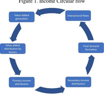
The interest in a country's economic problems and the need to solve questions about the effects of policies on the economic system are the basis for the development of research on Input-Output models. From this point of view, multisectoral models, disaggregated in terms of production typology and Institutional Sectors, represent a tool for economic policy analysis, as they are able to capture the disaggregated effect of the policies themselves and to simulate the effects of targeted interventions at sector level.In their extended form, the models are calibrated on the social accounting matrix (SAM), and are therefore able to capture the circularity of income, from its formation, to its primary allocation and secondary distribution, up to its use as final demand, as shown in the Figure 1

(16)

16

Under particular assumptions, which will be presented during the discussion of this chapter, the extended multisectoral model can be restructured in the form of "inoperability", which allows a specific analysis of anomal functioning production economic system, expressed as a percentage of its planned production capacity (Santos and & Haimes, 2004).

2. Framework of the Italian economy

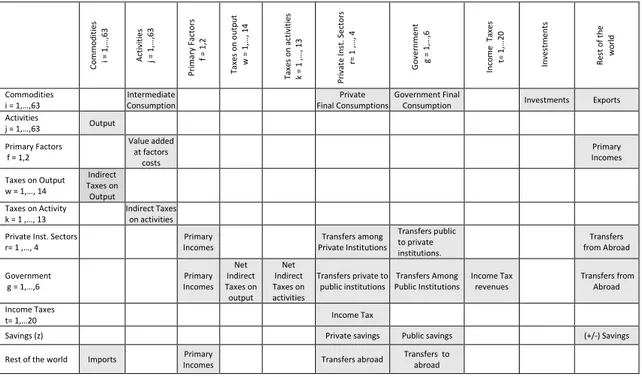
The application of the extended multisectoral models is referred to a benchmark given by the quantitative representation of the complete circular flow at a given time. The introduction of the policy measures for the containment of the contagion will determine deviations from the benchmark, providing results of the impacts on the macroeconomic variables. The Social Accounting Matrix, SAM, provides a most flexible accounting scheme especially suitable for representing the social and economic situation in its complexities. All the economic flows, among the various types of operators, are allocated according to their several origins and destinations, quantitatively corroborating the major logical links within the economy. Then, the SAM records the flows acting among operators in the various stages of the circular flow of income: production, value added generation, primary allocation of incomes, secondary distribution of incomes, income uses and accumulation, putting in evidence the multisectoral flow circularity. Its specific characteristics emphasise the general quantitative picture of the stages through which economic values originate and close to restart: production, among industries, value added according industries and value added components, income distribution, according value added components and institutions, income redistribution among institutions, and final demand by institutions and commodities. The scheme of the SAM for the year 2016 is shown in Figure 2.

(17)

17

Figure 2. Social Accounting Matrix and interactions among Institutional Sectors

The SAM for 2016 is characterized by 63 industries and 63 commodities ((complete list is available in Appendix 1); 2 primary factors, Labour and Capital; 4 private Institutional Sectors (Non-financial corporations, Financial corporations, Households, Non-profit institutions). Public administration is divided into 6 institutions (Central Government, Social Security Administration, Regional, Provincial and Communal governments, Other central administrations). The Rest of the World completes the set of Institutional Sectors.

SAM includes 20 different income taxes, 14 taxes on production and 13 taxes on activities included VAT, IRAP and Social Benefits.

The construction of the SAM started from the structure of the Input-Output table for the year 2016 produced by the National Institute of Statistics (ISTAT)2, and the ISTAT data for what concerns the primary distribution of income3.

2_{https://www.istat.it/it/archivio/238228} 3_{http://dati.istat.it/} C o mmo d it ies i = 1 ,… ,6 3 Act iv it ies j = 1 ,… ,6 3 Pr ima ry Fact o rs f = 1 ,2 T ax es o n o u tp u t w = 1 ,… , 1 4 Tax es o n act iv it ies k = 1 ,… , 1 3 Pr iv at e In st . Se ct o rs r= 1 ,… , 4 G o ver n ment g = 1 ,… ,6 In co me T ax es t= 1 ,… 2 0 In ves tm en ts Res t o f th e w o rl d Commodities i = 1,…,63 Intermediate Consumption Private Final Consumptions Government Final

Consumption Investments Exports Activities j = 1,…,63 Output Primary Factors f = 1,2 Value added at factors costs Primary Incomes Taxes on Output w = 1,…, 14 Indirect Taxes on Output Taxes on Activity k = 1 ,…, 13 Indirect Taxes on activities Private Inst. Sectors

r= 1 ,…, 4 Primary Incomes Transfers among Private Institutions Transfers public to private institutions. Transfers from Abroad Government g = 1,…,6 Primary Incomes Net Indirect Taxes on output Net Indirect Taxes on activities Transfers private to public institutions Transfers Among Public Institutions Income Tax revenues Transfers from Abroad Income Taxes t= 1,…20 Income Tax

Savings (z) Private savings Public savings (+/-) Savings

(18)

18

For taxes on commodities and industries, data published by ISTAT with details of taxes by item and by type of administration (central or peripheral) were used.The total was then distributed on the basis of the tax type, where a particular activity is identified, or on the basis of Value Added shares, where there is no specific and univocal reference. To strengthen the imputation methodology, data on tax returns have also been downloaded from the Department of Finance's website4, providing details by macro-sector of economic activity. Data on total taxes were also checked for those obtained from the RGS-ISTAT SIOPE database on public administrations' home flows, which provides details on the type and location of PA. With regard to income taxes, the detail produced by ISTAT was used. The transfers were estimated on the basis of the SIOPE data previously called up and checked for the RGS Statistical Yearbook data Table 2.2.5: Final allocations and results of State budget management by title and economic category. Finally, ISTAT's 2016 Institutional Accounts were used to check the consistency of the overall framework, especially with reference to gross savings.

3. Disaggregated income circular flow approach

Economic analysis of pandemics, in particular on the forecasted effects of policies aimed at its containment, find space in the literature, especially on the topics of the method of estimation proposed. The availability of contributions on evaluation tools has significantly expanded in recent years. The models used for impact analysis rely on sophisticated techniques of parametrization and validation; some of them incorporate elements that refer to the behaviour of individuals. In a recent work performed through a meta-analysis of the contributions in this field (Carrasco et al., 2013), emerge how the most commonly used models are the Agent-Based, the CGE and Network models. Further

(19)

19

contribution have been provided by the utilization of cost-benefit analysis where, given a predetermined project all costs and benefits directly or indirectly attributable to the project are taken into consideration.

In this work, an extended multisectoral model of inoperability is developed with the aim of providing an evaluation of the macroeconomic components’ impact of COVID-19 pandemic, living aside, for the moment, the policy activated for its containment.

Multi-sectoral models represent a valid tool for the analysis of direct and indirect effects on the economic system of policy measures, or spontaneous variations of a selective nature, i.e. phenomena that do not affect demand or supply as a whole. This type of policy includes the containment of contagions implemented by the Italian Government through the lockdown in which only the activities considered non-essential suffered the interruption of production, while the production of necessities remained unchanged. However, through sectoral interdependencies, among productive activities and among Institutional Sectors, the policy impacts on the entire economic system, affecting in the case of lockdown also the sectors not targeted by the policy.

This chapter aims to assess the effects of the lockdown policy through the application of an Extended Multisectoral model, highlighting the importance of the impact multipliers and Linkages, with the aim of identifying the productive activities with the greatest transfer effect to the economic system and the most important Institutional Sectors.

The Extended Multisectoral models represent an expansion of the Miyazawa model (Miyazawa, 1970), since final demand is completely endogenized5. Rather than concentrating only on consumption expenditures, also income transfers are taken into explicit consideration. This operation is performed through an extension of the model that

(20)

20

comprehends the behaviours of the institutions that determine primary and secondary distribution of incomes. All the relations between income generation, primary income allocation, secondary income distribution and the related formation of final demand are modelled through a linear system.This type of model also considers fixed prices, which implies that policy simulations do not allow evaluating the inflationary effect. These assumptions will be relaxed in the following chapters.

The accounting identity that shows, for each “i” commodity6, the available output and its destinations is written as:

𝐦 + 𝐪 ≡ 𝐫 + 𝐟 (1)

where m(i×1) is the imports vector, q(i×1) the domestic total output vector, r(i×1) the vector of domestic absorption of intermediate materials and f(i×1) the final demand vector. Final demand is given by the sum of its domestic components i.e. final consumptions, public expenditures, investments and exports. According their role in the model, however, final demand components are either endogenous 𝐟_𝐄 or exogenous 𝐟_𝐗

𝐟 = 𝐟𝐄+ 𝐟𝐗 (2)

Substituting eq. (2) into eq. (1) we get:

𝐦 + 𝐪 ≡ 𝐫 + 𝐟_𝐄+ 𝐟_𝐗 (3)

Total final output then results as the sum of intermediate endogenous and exogenous demands, which in the usual case consists of exports, minus imports:

𝐪 = 𝐫 + 𝐟_𝐄+ 𝐟_𝐗− 𝐦 (4)

Considering an open economy characterized by “i” types of commodities and by “j” activities producing them vector r of intermediate commodity consumptions can be written as:

𝐫 = 𝐀 𝐪 (5)

(21)

21

Matrix of technical coefficients A(i×i) is built as the product of matrix 𝐁 = 𝐔 𝐱̂−𝟏_,

sometimes called the Use matrix, that provides the amount of use of the ith commodity exhibited by the jth industry with the Make, or supply, matrix 𝐃 = 𝐕 𝐪̂−𝟏_{, that gives the}

shares of fabrication of commodity “i” provided by industry “j”.

Putting

𝐟𝐃 = 𝐟𝐄− 𝐦 (6)

which gives net endogenous demand and substituting eq. (5) and (6) in eq. (4), we get:

𝐪 = 𝐀 𝐪 + 𝐟_𝐃+ 𝐟_𝐗 (7)

In an economy characterized by s Institutional Sectors final demand represents the utilization of income and is tied to total output q through disposable income y of the same Institutional Sectors. Consequently, we need to design the entire process of distribution and redistribution of incomes. Starting from the vector of value added generated by each commodity vi we can write:

𝐯_𝐢 = 𝐋𝐪 (8)

where L(i×i) is a diagonal matrix whose diagonal element is determined as column sum of matrix (I-A). This allows for the determination of the vector of value added by commodity, vi (i×1). The vector of value added according the industry origin can be transformed into the vector of value added by destination, vc(c×1), i.e. by VA components, c, though the use of matrix W(c×i) from the IO table. We get:

𝐯_𝐜= 𝐖 𝐯_𝐢 (9)

where matrix W(c×i) gives the share of value added generated in each commodity that has been attributed to each VA component. The generation and primary distribution of income concludes with the attribution of the VA categories to the Institutional Sectors, i.e those sectors that are entitled to decide on the destination of income. Value added components are then attributed the institutions owner. Compensation of employees,

(22)

22

capital incomes, taxes on activities and indirect taxation contribute to the formation of the vector of primary balances:

𝐯_𝐬 = 𝐏 𝐯_𝐜 (10)

where matrix P(s×c) is the matrix of the primary distributive shares of Value Added by Institutional Sector and 𝐯𝐬(s×1).

The secondary distribution of incomes leads to the determination of the disposable incomes by institutions, 𝐲s(s×1), through the analysis of all interrelation among

Institutional Sectors and refers to unilateral income transfers both voluntary or required.

𝐲_𝐬 = (𝐈 + 𝐓) 𝐯_𝐬 (11)

where 𝐈(s×s) is a unit matrix and 𝐓(s×s) the transfer income shares among Institutional Sectors by each institution. Substituting eq. (8) (9) and (10) in eq. (11) we get the disposable income vector of Institutional Sectors, ys (s×1) expressed as a function of the total output vector:

𝐲𝐬 = [(𝐈 + 𝐓) 𝐏 𝐖 𝐋] 𝐪 (12)

Matrix C(s×s) is a diagonal matrix of the average consumption propensity of each Institutional Sector, so that matrix (I-C) represents the savings propensity of the Institutional Sectors. Matrix 𝐒(s×s) represents the active saving, the ratio between savings of Institutional Sectors, with exclusion of the rest of the world, and investment expenditures of Institutional Sectors as they emerge from the Social Accounting Matrix. Matrix M(s×s) is a diagonal matrix of the average import propensity, equal for each Institutional Sector; it is obtained through the ratio between total imports and the total disposable income of Institutional Sectors.

We define matrix G(i×s) as the product of matrices F and C plus the matrix obtained as 𝐊 𝐒(𝐈 − 𝐂) less matrix ZM. The matrix F(i×s) gives the shares of final consumption by commodity with respect to the total consumption expenditure of Institutional Sectors;

(23)

23

matrix K(i×s) transforms investment by Institutional Sectors into investment by commodity; finally, matrix Z(i×s) represents the shares of imports by commodity

𝐆 = 𝐅 𝐂 + 𝐊 𝐒 (𝐈 − 𝐂) − 𝐙𝐌 (13)

Endogenous final demand can be then determined as:

𝐟𝐃 = 𝐆 [(𝐈 + 𝐓) 𝐏 𝐖 𝐋]𝐪 (14)

Substituting eq, 14 in eq. 7 we get:

𝐪 = 𝐀 𝐪 + 𝐆 [(𝐈 + 𝐓) 𝐏 𝐖 𝐋] 𝐪 + 𝐟𝐗 (15)

Putting 𝐄 = 𝐆 [(𝐈 + 𝐓)𝐏 𝐖 𝐋] 𝐪 gives:

𝐪 = 𝐀 𝐪 + 𝐄 𝐪 + 𝐟_𝐗 (16)

The resulting reduced form of the extended I-O, which includes the income distribution process and final demand formation will be given by:

𝐪 = [𝐈 − 𝐀 − 𝐄]−𝟏 𝐟𝐗 (17)

or alternatively

𝐪 = 𝐑 𝐟_𝐗

where total-output vector q represents the expected results to be attained. Of course, results for all the other variables can be determined using the convenient set of matrices. In the case of expected results on value-added we can easily substitute eq. (17) in eq. (8) and get:

𝐑_𝐕𝐀 = 𝐋 𝐪 = 𝐋𝐑 (18)

Through the R matrix it is therefore possible to calculate the impact multipliers considering the column or row sum; the R matrix is a square matrix commodity by commodity with size (i×i), and therefore a transformation of the second subscript is necessary in order to differentiate row totals from column totals; for this reason it is assumed that:

(24)

24

𝐑(𝒊 × 𝒊) = 𝐑(𝒊 × 𝒌) with k = i The impact multipliers are therefore obtained as follows:

Ok= ∑ rik n

i=1

(19)

where, for example, the multipliers 𝑂1 corresponds to the effect on total production as a

result of a unitary increase in exogenous final demand of the production activity 1; on the contrary:

Oi = ∑ rik n

k=1

(20)

detects the increase in output of product 1 necessary to meet an increase in exogenous final demand for all products.Through a standardisation process on the average of impact multipliers it is also possible to construct two types of indexes, Backward and Forward, which respectively highlight the products that register a greater increase in output and input, with respect to the others7, following a unitary increase in demand for a product. Indicating with: µ_𝑘 =∑ 𝑟𝑖𝑘 𝑛 𝑖=1 𝑛 µ_𝑖 =∑ 𝑟𝑖𝑘 𝑛 𝑘=1 𝑛 μ =∑ ∑ rik n k=1 n i=1 N Backward and Forward linkages are calculated as:

Back_k= µk

μ (21)

7_{When an Backward or Forward linkage for commodity “i” assumes a value greater than 1, it means that}

the increase in output of the “i” commodity is greater than all the others, and vice versa when it assumes a value less then 1.

(25)

25

For_i =µi

μ (22)

Since these indices are based on the average, it is necessary to calculate a dispersion index that allows to analyse the distribution of multipliers within the vector of each commodity. In this way, low variability corresponds to a homogeneous distribution of the multiplicative effect between all products, and vice versa. The index used is the coefficient of variation because, since it is a non-dimensional index, it allows comparing measurements of different sizes. The coefficient of variation for backwards and forward linkages are calculated as follows

σ_k= √∑ (rij− µk) 2 n i=1 n − 1 µ_k (23) σ_i = √∑ (rij− µi) 2 n k=1 n − 1 µ_k (24)

4. Supply shock and the Extended Multisectoral Inoperability Model

The Inoperability Input Output Model (IIM) is used for evaluating the impacts that events of great magnitude, as pandemic, can create in the economic system, as in (Santos and Haimes, 2004; Leugh et al., 2007) where the authors evaluate the economic impact of a terrorist attack. IIM is based on the results of Input-Output Leontief model, as the expected results of the physiological performance of the interindustry interactions and the actual results of unexpected locks in the delivery-flows of intermediate interactions. As seen above, when analysing highly interconnected components in an input-output (I-O) framework, an important concept is that of the key sector describing the influence of a product or an industry on the expansion of the whole economic system

(26)

26

(Lahr and Dietzenbacher, 2001). Clearly this assumption becomes more relevant in a SAM context, where the concept of the key production sector is extended also to the Institutional Sectors. From this point of view, production interruptions in key sectors deriving from a large-scale exogenous event, such as natural disasters and pandemics, can generate amplified effects that the extended multisectoral model in its classical formulation is unable to capture. Consequently, through the application of the concept of inoperability to extended multisectoral models (EIIM) (Ciaschini et al, 2018) it is possible to carry out an analysis of the effects that a major exogenous event can have both on the production system and on the formation, distribution and redistribution of income. Under physiological conditions, the economy attains the expected results. In this case, where no interruptions in the deliveries are observed we can determine a matrix of the corresponding market shares well-matched with the given set of technical coefficients. The structure of intermediate deliveries of the output of each industry jth to the ith industry is represented by set of ratios (𝑞𝑗

𝑞𝑖) for i=1…,n and j=1…,n. Multiplying these ratios by

the corresponding constant technical coefficient, 𝑎𝑖𝑗, we obtain the market share, 𝑎𝑖𝑗∗, of

all industry-outputs with respect to the industry that produces commodity i, i.e.: 𝑎_𝑖𝑗∗ = 𝑎_𝑖𝑗(𝑞𝑗

𝑞_𝑖)

The matrix of the market shares will be then given by:

A∗ = [ 𝑎11( 𝑞₁ 𝑞₁) 𝑎12( 𝑞₂ 𝑞₁) ⋯ 𝑎1𝑛( 𝑞_𝑛 𝑞₁) ⋮ ⋮ ⋮ 𝑎_𝑛1(𝑞1 𝑞_𝑛) 𝑎𝑛2( 𝑞₂ 𝑞_𝑛) ⋯ 𝑎𝑛𝑛( 𝑞_𝑛 𝑞_𝑛)] (25)

In fact, since the technical coefficient is defined as the intermediate flow Mij divided by

the output of industry of destination:

𝑎_𝑖𝑗 =𝑀𝑖𝑗 𝑞_𝑗

(27)

27 It is possible to obtain: A∗ = [ 𝑀₁₁(1 𝑞₁) 𝑀12( 1 𝑞₁) ⋯ 𝑀1𝑛( 1 𝑞₁) ⋮ ⋮ ⋮ 𝑀_𝑛1(1 𝑞_𝑛) 𝑀𝑛2( 1 𝑞_𝑛) ⋯ 𝑀𝑛𝑛( 1 𝑞_𝑛)] (26)

where each element is the intermediate flow, Mij, weighted according the output level of

the industry of origin, which is indeed the definition of intermediate market share of commodity i.

Under exceptional events some industries or all the industries in the economy undergoes a loss in output that will prevent the expected deliveries to industries take place. Then, it is possible to write 𝐀∗ matrix (25) as a transformation of the technical coefficient matrix A. Operator ‘^’ (e.g. q̂ ) gives an (n×n) diagonal matrix where the elements of vector q appear on the main diagonal and zeros are elsewhere. The logical link between matrix 𝐀∗ of the market shares and the Leontief coefficients matrix, A, then, is as follows:

𝐀∗ _{= 𝐪}_̂−𝟏_{𝐀 𝐪}_̂ ₍₂₇₎

Let’s denote with q̃I the actual total output deliveries of industry i, after the

lockdown, in a context where the capability of commodity i to comply with the demands of the industries is weakened. The difference between the expected value and the actual value will determine the inoperability of the ith industry:

z_i = qi− q̃i

q_i (28)

In matrix form:

(28)

28

On the other hand, the obstruction of final demand can be expressed by vector 𝐟∗_,

whose elements are a function of the difference between the levels of expected demand and the levels actually attained by final demand in the inoperability situation. The economy can experience an unexpected reduction in demand following an interruption for various reasons as the result of diminished supply and or because of the persistent consumer concern on future events as well as safety apprehensions.

The normalized losses of exogenous final demand for each commodity are represented by scalars f_i∗, determined as the ratio between the expected final demand net of actual demand and expected total output. The contraction due to the catastrophic event, and the potential total output:

f_i∗ = fi− f̃ i qi

i = 1,..,n (30)

or in matrix form:

𝐟∗ = 𝐪̂−𝟏_(𝐟 _{− 𝐟̃}₎ ₍₃₁₎

The inoperability model can be written as:

𝐳 = 𝐀∗ 𝐳 + 𝐟∗ (32)

The Inoperability Extended Multisectoral Model, IEMM, is designed on the basis of the demand-oriented IIM, integrating in the inoperability process endogenous demand and income transfers among institutions (Ciaschini et al., 2018). We design an 𝐄∗ matrix of the loop income distribution/final demand formation, similar to matrix E. This matrix however is obtained substituting diagonal matrix L, that determines the Value Added vector given total output, with matrix L*_{whose diagonal elements are taken as}

column-sums of matrix 𝐀∗_{of the market shares. Then, putting 𝐄}∗ _{= 𝐆 [(𝐈 + 𝐓)𝐏 𝐖 𝐋}∗_{] and:}

𝐟_𝐗∗ = 𝐪̂−𝟏_(𝐟

𝐗− 𝐟̃ ) 𝐗 (33)

(29)

29

𝐳 = 𝐀∗_{𝐳 + 𝐄}∗_{𝐳 + 𝐟}

𝐗∗ (34)

or in the reduced form:

𝐳 = [𝐈 − 𝐀∗− 𝐄∗]−𝟏_𝐟

𝐗∗ (35)

The effects on value added are determined through matrix L*: 𝐯_𝒊∗= 𝐋∗_{𝐳 = 𝐋}∗_{[𝐈 − 𝐀 − 𝐄}∗_]−𝟏_𝐟

𝐗∗ (36)

where v_𝑖∗ is the value added inoperability as share of total output.

5. Key industries in EMM

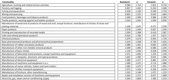
Table 1 shows the results of Backward and Forward linkages and the relative coefficients of variation calculated on the R matrix for the Italian SAM. It is possible to observe that the best combination between the two indices, i.e. the maximum distance between the linkages and the coefficient of variation, is associated with the products "Air transportation" and "Water transportation", followed by the products "Repair and installation services of machinery and equipment" and "Travel agency, tour operator reservation service and related activities". Figure 3 shows the products with the greatest multiplicative effect, regardless of the level of variation.

Table 1. Backward and Forward linkages

Commodity Backward σ Forward σ

Agriculture, hunting and related service activities 0.980 1.753 1.815 0.743

Forestry and logging 0.897 1.642 0.250 5.000

Fishing and aquaculture 0.938 1.520 0.240 4.793

Mining and quarrying 0.892 1.591 0.643 1.864

Food products, beverages and tobacco products 1.040 _1.999 3.986 0.383 Textile products, wearing apparel and leather products 1.024 1.942 1.694 0.995 Manufacture of wood and of products of wood and cork, except furniture; manufacture of articles of straw and

plaiting materials 1.048 1.625 0.472 3.209

Paper products 1.078 1.569 0.607 2.456

Printing and reproduction of recorded media 1.039 1.398 0.410 2.907 Coke and refined petroleum products 0.924 1.706 1.437 0.871

Chemical products 1.079 1.674 0.945 1.724

Basic pharmaceutical products and pharmaceutical preparations 1.010 1.568 0.730 1.816 Manufacture of rubber and plastic products 1.080 1.461 0.692 1.878 Manufacture of other non-metallic mineral products 1.049 1.485 0.586 2.245

Manufacture of basic metals 1.139 1.658 0.358 4.993

Manufacture of fabricated metal products, except machinery and equipment 1.071 1.606 1.255 1.193 Manufacture of computer, electronic and optical products 1.007 1.490 0.655 1.906 Manufacture of electrical equipment 1.089 1.477 0.485 2.876 Manufacture of machinery and equipment n.e.c. 1.089 1.475 0.714 1.886 Manufacture of motor vehicles, trailers and semi-trailers 1.085 1.475 0.735 1.855 Manufacture of other transport equipment 1.072 1.416 0.358 3.634 Manufacture of furniture, other manufacturing 1.032 1.548 1.071 1.225 Repair and installation services of machinery and equipment 1.050 1.371 0.677 1.684 Electricity, gas, steam and air conditioning supply 1.056 1.804 1.584 1.014

(30)

30

Water supply, sewerage, waste management and remediation activities 0.985 1.422 0.310 3.665 Sewerage, waste collection, treatment and disposal activities, materials recovery, remediation activities and other

waste management services 1.003 1.590 0.923 1.448

Construction 1.036 1.882 3.744 0.380

Wholesale and retail trade services, repair of vehicles and motorcycles 1.015 _1.410 0.619 1.832 Wholesale trade, except of motor vehicles and motorcycles 1.004 1.461 0.608 1.950 Retail trade, except of motor vehicles and motorcycles 0.967 1.465 0.143 7.937 Land transport and transport via pipelines 1.035 1.570 1.047 1.256

Water transport 1.049 1.346 0.200 5.675

Air transport 1.059 _1.321 0.225 5.038

Warehousing and support activities for transportation 1.014 1.661 1.133 1.238

Postal and courier activities 1.017 1.437 0.259 4.500

Accommodation and food service activities 0.980 1.729 2.594 0.441

Publishing activities 1.009 1.427 0.446 2.634

Motion picture, video and television programme production, sound recording and music publishing activities,

programming and broadcasting 1.021 1.516 0.431 3.044

Telecommunications 0.983 1.671 0.821 1.678

Computer programming, consultancy and related activities, information service activities 0.987 1.642 1.251 1.034 Financial service activities, except insurance and pension funding 0.925 1.701 1.518 0.804 Insurance, reinsurance and pension funding, except compulsory social security 0.956 1.605 0.747 1.612 Activities auxiliary to financial services and insurance activities 0.968 1.557 0.757 1.649

Real estate activities 0.887 1.995 4.663 0.239

Legal and accounting activities, activities of head offices, management consultancy activities 0.933 1.704 1.822 0.665 Architectural and engineering activities, technical testing and analysis 1.009 1.489 0.865 1.356 Scientific research and development 0.989 1.467 0.794 1.441

Advertising and market research 1.037 1.392 0.509 2.274

Other professional, scientific and technical activities, veterinary activities 0.969 1.486 0.530 2.173

Rental and leasing activities 1.008 1.440 0.679 1.734

Employment activities 0.907 1.563 0.302 3.745

Travel agency, tour operator reservation service and related activities 1.061 1.394 0.401 2.978 Security and investigation activities, services to buildings and landscape activities, office administrative, office

support and other business support activities 0.995 1.540 1.299 0.908 Public administration and defence, compulsory social security 0.910 1.748 2.650 0.422

Education 0.862 1.749 1.682 0.664

Human health activities 0.948 1.773 2.884 0.416

Social work activities 0.963 1.553 0.595 2.014

Creative, arts and entertainment activities, libraries, archives, museums and other cultural activities, gambling and

betting activities 0.960 1.690 0.929 1.437

Arts, entertainment and recreation 0.994 1.544 0.464 2.768 Activities of membership organisations 1.016 1.392 0.256 4.424 Repair of computers and personal and household goods 0.968 1.429 0.232 4.874 Other personal service activities 0.923 1.575 0.774 1.469 Activities of households as employers, undifferentiated goods- and services-producing activities of households for

own use 0.880 1.647 0.494 2.311

Figure 3. Backward linkages - 10 highest values

It should be noted that the greatest multiplier effect is associated with the commodities "Manufacture of basic metals" and "Manufacture of electrical equipment". To these

Manufacture of basic metals Manufacture of electrical equipment Manufacture of machinery and equipment n.e.c. Manufacture of motor vehicles, trailers and semi-trailers Manufacture of rubber and plastic products Chemical products Paper products Manufacture of other transport equipment Manufacture of fabricated metal products, except machinery and equipment Travel agency, tour operator reservation service and related activities Backward linkages 1,139 1,089 1,089 1,085 1,080 1,079 1,078 1,072 1,071 1,061 1,020 1,040 1,060 1,080 1,100 1,120 1,140 1,160

(31)

31

sectors are associated a higher level of the coefficient of variation, and this indicates, as mentioned above, that the multiplication effect of these commodities on all the others is not equally distributed. Therefore these are more related to some commodities than to others. Observing the composition of the impact multiplier vector associated with the "Manufacture of electrical equipment" product, it is possible to note that the distribution is not homogeneous, but the product is strongly connected with the "Real estate activities" (c44), "Food products, beverages and tobacco products" product. (c5) and "Construction" (c27).

Figure 4. Multiplier impact of “Manufacture of basic metals”

Figure 5 shows the commodities with the lowest multiplicative impact, particularly associated with the commodity “Education” e “Activities of households as employers, undifferentiated goods- and services-producing activities of households for own use”.

As regards to the Forward linkages, observing the Table 1, it is possible to note that the commodities with the greatest multiplicative effect and at the same time with less

0,000 0,050 0,100 0,150 0,200 0,250 0,300 0,350 0,400 0,450 0,500 c1 c3 c5 c7 c9 _c11 _c13 _c15 _c17 _c19 _c21 _c23 _c25 _c27 _c29 _c31 _c33 _c35 _c37 _c39 _c41 _c43 _c45 _c47 _c49 _c51 _c53 _c55 _c57 _c59 _c61 _c63

(32)

32

variability are "Real estate activities" and "Food products, beverages and tobacco products".

Figure 5. Backward linkages - 10 lowest values

Looking at Figure 6, these commodities, unlike what observed for Backward linkages, really have the greatest multiplicative effect compared to the others, and this implies that this type of product plays an important role as a supplier sector of the economic system.

Figure 6. Forward linkages - 10 highest values

Finally, in Figure 7 it is possible to observe the commodities with the lowest multiplicative impact in terms of forward linkages; in particular, there is a low

Education Activities of households as employers, undifferentia ted goods-and services-producing activities of households for own use

Real estate activities Mining and quarrying Forestry and logging Employment activities Public administrati on and defence, compulsory social security Other personal service activities Coke and refined petroleum products Financial service activities, except insurance and pension funding Backward linkages 0,862 0,880 0,887 0,892 0,897 0,907 0,910 0,923 0,924 0,925 0,830 0,840 0,850 0,860 0,870 0,880 0,890 0,900 0,910 0,920 0,930 Real estate activities Food products, beverages and tobacco products Construction Human health activities Public administrati on and defence, compulsory social security Accommodat ion and food service activities Legal and accounting activities, activities of head offices, management consultancy activities Agriculture, hunting and related service activities Textile products, wearing apparel and leather products Education Forward linkages 4,663 3,986 3,744 2,884 2,650 2,594 1,822 1,815 1,694 1,682 0,000 0,500 1,000 1,500 2,000 2,500 3,000 3,500 4,000 4,500 5,000

(33)

33

multiplication effect with regard to the commodities "Retail trade, except of motor vehicles and motorbikes" and "Water transport".

Figure 7. Forward linkages - 10 lowest values

6. Structural changes and optimal endogenous policy tools

As seen in the previous paragraphs, through the multipliers’ analysis it is possible to obtain information on the increase in sectoral production resulting from unitary shock of a single commodity demand. However, the hypothesis of a unitary shock does not apply in economic reality (Ciaschini, 1988a), but on the contrary, the increase or decrease in demand for commodities is due to a structure that is not necessarily uniformly distributed (Socci, 2004). Therefore, it is necessary to search for the optimal structure that generates the maximum multiplicative effect; this structure can be reconstructed by using the Single Value Decomposition applied to the matrix of multipliers.This methodology is based on the decomposition of the matrix of multipliers into 3 matrices made up respectively of the left eigenvectors, the singular values and the right eigenvectors:

𝐑 = 𝐔 𝐒 𝐕′ ₍₃₇₎ Retail trade, except of motor vehicles and motorcycles Water

transport Air transport Repair of computers and personal and household goods Fishing and aquaculture Forestry and logging Activities of membership organisation s Postal and courier activities Employment activities Water supply, sewerage, waste management and remediation activities Forward linkages 0,143 0,200 0,225 0,232 0,240 0,250 0,256 0,259 0,302 0,310 0,000 0,050 0,100 0,150 0,200 0,250 0,300 0,350

(34)

34

where U(i×k) is the left eigenvector matrix, S(i×k) is a diagonal matrix of singular values8, sorted in descending order, named macro multipliers, and V’(k×i) is the right eigenvectors matrix. The decreasing structure of the singular value matrix indicates the decreasing effect of the incoming structures dictated by the incoming (right eigenvectors) and outgoing (left eigenvectors). Therefore, the structure associated with the first vector of the right eigenvector matrix has the greatest multiplicative effect and returns the output structure dictated by the first vector of the left eigenvector matrix:

𝐑_𝟏= 𝐮_𝟏 𝐬_𝟏 𝐯_𝟏 (38)

Consequently, vector v1 can be considered as the multiplier optimal structure. The R1

matrix represents the matrix of multipliers associated with an exogenous final demand shock with v1 structure.It is clear that the sum of the single matrices calculated through

the incoming singular vector corresponds to the R matrix, that is to say R = ∑ R_i

i

(39)

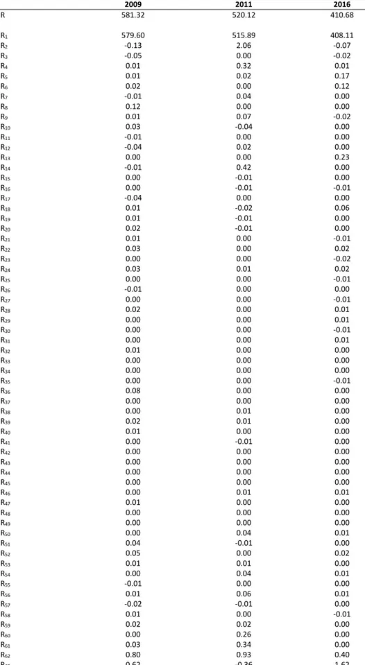
Applying the breakdown to the R matrices calculated on the Italian SAMs of 2009, 2011 and 20169, it is possible to obtain the multiplicative effect of the individual Ri matrices (see Table 2). From the table, it can be seen that the effect is reduced in the transition from SAM 2009 to SAM 2016; it is also evident how the first singular value, associated with the first incoming and the first outgoing car, captures almost the totality of the general multiplicative effect, making the multiplicative structures of the other vectors negligible.

8_{Singular values are calculate as the square root of eigenvalues, 𝑠}

𝑖= √𝜆𝑖

(35)

35

Table 2. Singular Value Decomposition on R matrix and multiplier effects

2009 2011 2016 R 581.32 520.12 410.68 R1 579.60 515.89 408.11 R2 -0.13 2.06 -0.07 R3 -0.05 0.00 -0.02 R4 0.01 0.32 0.01 R5 0.01 0.02 0.17 R6 0.02 0.00 0.12 R7 -0.01 0.04 0.00 R8 0.12 0.00 0.00 R9 0.01 0.07 -0.02 R10 0.03 -0.04 0.00 R11 -0.01 0.00 0.00 R12 -0.04 0.02 0.00 R13 0.00 0.00 0.23 R14 -0.01 0.42 0.00 R15 0.00 -0.01 0.00 R16 0.00 -0.01 -0.01 R17 -0.04 0.00 0.00 R18 0.01 -0.02 0.06 R19 0.01 -0.01 0.00 R20 0.02 -0.01 0.00 R21 0.01 0.00 -0.01 R22 0.03 0.00 0.02 R23 0.00 0.00 -0.02 R24 0.03 0.01 0.02 R25 0.00 0.00 -0.01 R26 -0.01 0.00 0.00 R27 0.00 0.00 -0.01 R28 0.02 0.00 0.01 R29 0.00 0.00 0.01 R30 0.00 0.00 -0.01 R31 0.00 0.00 0.01 R32 0.01 0.00 0.00 R33 0.00 0.00 0.00 R34 0.00 0.00 0.00 R35 0.00 0.00 -0.01 R36 0.08 0.00 0.00 R37 0.00 0.00 0.00 R38 0.00 0.01 0.00 R39 0.02 0.01 0.00 R40 0.01 0.00 0.00 R41 0.00 -0.01 0.00 R42 0.00 0.00 0.00 R43 0.00 0.00 0.00 R44 0.00 0.00 0.00 R45 0.00 0.00 0.00 R46 0.00 0.01 0.01 R47 0.01 0.00 0.00 R48 0.00 0.00 0.00 R49 0.00 0.00 0.00 R50 0.00 0.04 0.01 R51 0.04 -0.01 0.00 R52 0.05 0.00 0.02 R53 0.01 0.01 0.00 R54 0.00 0.04 0.01 R55 -0.01 0.00 0.00 R56 0.01 0.06 0.01 R57 -0.02 -0.01 0.00 R58 0.01 0.00 -0.01 R59 0.02 0.02 0.00 R60 0.00 0.26 0.00 R61 0.03 0.34 0.00 R62 0.80 0.93 0.40 R63 0.62 -0.36 1.62

(36)

36

7. Supply side shock and Covid-19

With the Prime Minister’s Decree DPCM 22th_{march 2020, regarding “Urgent}

measures for containment of infection by coronavirus on the whole national territory”, Government has determined the lockdown of all “non-essential” activities, listed in the attachment 1 of the same DPCM, further modified with the decree of the Ministry of economic development 25th march 2020.

With the decree, the shutdown of 57% of industrial activities has been decided. The remaining 43% of industries has continued to produce, albeit with less intensity with respect to the pre-COVID period, given the final demand fall, difficulties in logistics and the partial lock in the main foreign partners with some exceptions as for the pharmaceutical and food industries10. A policy action, then, of relevant magnitude actually limiting the supply side. Since the measure is tied to the containment of the contagion, the date of reopening the activities is not unique, but established from time to time, for the various industries, according the evolution of the pandemic.

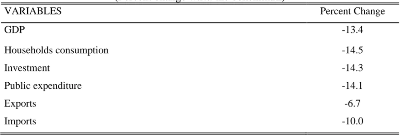
The shutdown of “non-essential” activities results in an actual reduction of yearly total output of around three months’ loss of actual total output on yearly basis. In addition, for transport sectors, Hotels, catering services and entertainment activities, the lockdown is extended to five months. This reveals as an output contraction of 14%.

The problem is then that of establishing the impact that the shutdown will generate directly and indirectly on the value added generation, on disposable income formation of institutions, and on the utilization of disposable income.

In the simulation have been deliberately neglected the measure by Government to households support, as suspension of tax payments, financial supports, deferring tax

10_{Il Sole 24 ore -}

(37)

37

debts; actions that act as economic impact dampener to the output lockout through supporting aggregate final demand and triggering a redistribution process.

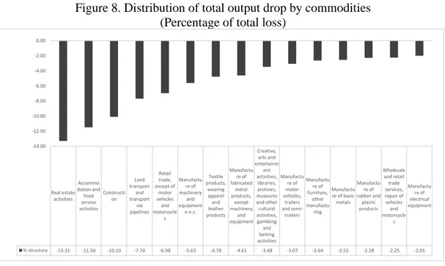
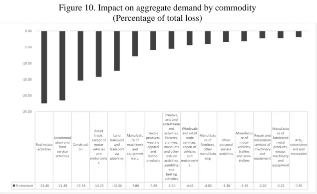
Figure 8 shows how the total output drop due to the shutdown policy results spread among commodity outputs.

Figure 8. Distribution of total output drop by commodities (Percentage of total loss)

The greatest contraction concentrates on Real estate activities and Accomodation

and food service activities, followed by Construction and Land transport and transport via pipelines. Real estate activities and Accomodation and food service activities

represent respectively 15.38% and 7.21% of total production, while Construction and

Land transport and transport via pipelines represent respectively 10.85% and 0.45%.

Therefore, the four industries represent 33.89% of total production, i.e. more than a third. Looking at the graph, 24.81% of the decrease in production is due to the drop in the Real

estate activities and Accommodation and food service activities sector and the 17.80% is

due to the drop in the Construction and Land transport and transport via pipelines, indicating that the 42.61% of the drop in production is due to these 4 sectors.

The total output contraction associated with the restriction measures preventing the COVID-19 spread, which impose the compulsory inactivity of a major part of the work

Real estate activities Accommo dation and food service activities Constructi on Land transport and transport via pipelines Retail trade, except of motor vehicles and motorcycle s Manufactu re of machinery and equipment n.e.c. Textile products, wearing apparel and leather products Manufactu re of fabricated metal products, except machinery and equipment Creative, arts and entertainm ent activities, libraries, archives, museums and other cultural activities, gambling and betting activities Manufactu re of motor vehicles, trailers and semi-trailers Manufactu re of furniture, other manufactu ring Manufactu re of basic metals Manufactu re of rubber and plastic products Wholesale and retail trade services, repair of vehicles and motorcycle s Manufactu re of electrical equipment % structure -13.31 -11.50 -10.10 -7.70 -6.98 -5.63 -4.78 -4.61 -3.48 -3.07 -2.64 -2.55 -2.28 -2.25 -2.01 -14.00 -12.00 -10.00 -8.00 -6.00 -4.00 -2.00 0.00

(38)

38

force, has a direct impact on factors’ demand by firms, causing a contraction in labour demand and a fall in investments.

As reported by the International Labour Organization (ILO) the policy affects immediately the quantity of labour, with a growth of unemployment and this implies a diminution of incomes of employees. In practice, these phenomena are damped by the operation of social safety nets and the extraordinary public policy measures planned. Since the aim of the research is that of isolating the actual economic damage of pandemic, the model operates without corrections.

In fact, concentrating on the impact that the health restrictions have at the level of disaggregated value added generation, in Table 1 is visible how the output contraction concentrates mainly the gross operating income and on employees incomes, as well as the drop in the government revenue.

Table 3. Impact on Value Added by components (Percent change w.r.t. the benchmark)

VALUE ADDED COMPONENTS %

Compensation of employees -11.7

Employer’s Social Contributions -10.8

Taxes on Output -16.0

Gross Operating Surplus -15.6

Indirect Taxes -10.5

Value Added Change -13.4

The selective shutdown of activities implies an aggregate contraction of employment income of 11.7%. Such a contraction can constitute the economic justification to the extension of the temporary lay-off scheme for employees by social security institutions to employees suspended by the work obligation, or with a reduced obligation. On the other hand, provisions concerning the contraction of capital remuneration should be utilized for activating the integration, at least partial, for the

(39)

39

remuneration of profit earners. In coherence with the reduction of total output, it is possible to observe the contraction of the tax revenue from taxes on activities, on outputs by the public Administration. Here are not considered provisions aimed to dampen the negative impacts on output and income given the aim to establish the economic impact of pandemic. With respect to disposable income of Institutional Sectors, given the value added reductions a reduction is also detected as reported in Table 3.

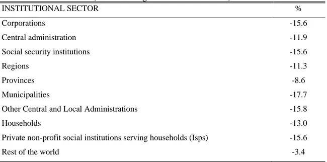
Total disposable income undergoes a decline of 13% consistent with the reduction of value added. A greater negative impact is registered in private Institutional Sectors, households and corporations, since they hold respectively 64.98% e 14.36% of disposable income. Such values as derived from the SAM, are displayed in Figure 9.

Figure 9. Impact on disposable income by Institutional Sector (Percentage of total loss)

The figure shows the negative impact of the health measures on disposable incomes of institutions. These incomes, in fact, do not only undergo the direct contraction, but also the negative effects of the contraction in transfers both to private and public institutions. The reduction of employees-incomes and capital-incomes, leads to a contraction of the tax base of private operators that generates i) a decline of indirect taxes paid to the public

Corporations _{administration}Central Social security_institutions Regions Provinces Municipalities

Other Central and Local Administrations Households Private non-profit social institutions serving households (Isps) Rest of the world % structure -14.36 -10.23 -0.17 1.56 -0.37 -2.08 -9.06 -64.98 -0.45 0.14 -70.00 -60.00 -50.00 -40.00 -30.00 -20.00 -10.00 0.00 10.00

COVID-19: TRADE-OFF BETWEEN HEALTH AND ECONOMICS

COVID-19: TRADE-OFF BETWEEN HEALTH AND ECONOMICS

Contents

Chapter 1

Covid-19 Pandemic and the supply side shock in Italy