A MODIFIED BESSEL DISTRIBUTION OF THE SECOND KIND Saralees Nadarajah
1. INTRODUCTION
Univariate Bessel function distributions are rapidly becoming distributions of first choice whenever “something” with heavier than Gaussian tails is observed in the data. They have been used to model: signal output processed by a radar re-ceiver under various sets of conditions (McNolty, 1967) and vibrational ampli-tude on the surfaces of ultrasonic transducers (Kielczynski and Pajewski, 1993; Kielczynski et al., 1993). They have also been used for modeling problems in ap-plied physics (Salingaros, 1991).
The two standard Bessel function distributions are the Bessel function distri-bution of the first kind and the Bessel function distridistri-bution of the second kind. The latter has the probability density function (pdf) given by
1 | | ( ) 2 ( 1/2) m m m m x x f x K b b m π +Γ ⎛ ⎞ = ⎜ ⎟ + ⎝ ⎠ (1)
for −∞<x<∞, b>0 and m>1, where
2 1/2 1 Γ ( ) ( 1) exp( ) 2 ( 1/2) m m m m π x K x t xt dt m ∞ − = − − +
∫
is the modified Bessel function of the second kind. Many generalizations of (1) have been proposed in the literature. See Harris and Soms (1974), Thabane and Kibria (1999), Anh et al. (2005), Gupta and Nadarajah (2006) and Srivastava and Nadarajah (2006). However, most of these generalizations are motivated by mathematical arguments, and not by statistical or physical needs. For example, the pdf of the distribution proposed in Srivastava and Nadarajah (2006) takes the form | |C x α K c x K d xm( | |) ( | |)n which has attractive mathematical properties.
The aim of this note is to introduce a modification of (1) that has real statistical motivation and to study its mathematical properties. Particularly, the new distri-bution is motivated by a Bayesian inference of an inverse Gaussian sample. An inverse Gaussian distribution is given by the pdf
2 2 3/2 ( ) ( ) exp 2 2 x -f x x x λ µ λ µ π ⎛ ⎞ = ⎜− ⎟ ⎝ ⎠ (2)
for x>0, λ>0 and µ>0, where λ is a reciprocal measure of dispersion and µ is a measure of location. Sometimes, it is more convenient to rewrite (2) as
2 3/2 exp( ) ( ) exp 2 2 2 x f x x x λ φ φ λ λ π ⎛ ⎞ = ⎜− − ⎟ ⎝ ⎠ (3)
where φ = λ/µ. The parameter φ determines the shape of the distribution and the pdf is highly skewed for moderate values of φ. As φ increases the inverse Gaus-sian tends towards the normal law.
The inverse Gaussian distribution is one of the most applied in the sciences. Areas of application include: actuarial science, analysis of reciprocals, demogra-phy, histomorphometry, electric networks, hydrology, life tests, management sci-ence, meteorology, mental health, physiology, remote sensing, traffic noise inten-sity, market research, regression, slug lengths in pipelines, ecology, entomology, small area estimation, CUSUM, and plutonium estimation. For details on the the-ory and applications of the distribution, we refer the reader to Chhikara and Folks (1989) and Seshadri (1998).
Suppose now we have a random sample x = (x1,...,xm) from (3) with
parame-ters (λ, φ). We wish to make inferences about the value of φ, e.g. H0 : φ =c versus
H1 : φ ≠c. The joint pdf of x is 2 /2 2 3/2 1 1 1 1 ( | , ) (2 ) exp( ) exp 2 2 m m m m m/ i i i i i i f m x x x φ λ λ φ π φ λ λ − − = = = ⎧ ⎫ ∝ Π ⎨− − ⎬ ⎩
∑
∑
⎭ x (4)Consider the prior pdf
1 2
( , ) exp( m n )
π λ φ ∝λ− − φ− φ , (5)
a diffuse prior in terms of λ and a normal in terms of φ. We obtain the joint pos-terior pdf as 2 /2 /2 1 3/2 2 1 1 1 1 ( , | ) (2 ) exp 2 2 m m m m m i i i i i i x n x x λ φ λ π λ φ π φ λ − − − = = = ⎧ ⎫ ∝ Π ⎨− − − ⎬ ⎩
∑
∑
⎭ x .Integrating out λ using equation (2.3.16.1) in Prudnikov et al. (1986, volume 1), we obtain the marginal posterior pdf of φas
/2 2 /2 1 1 1 ( | ) m exp( ) m m m i i j j n K x x π φ φ φ φ = = ⎛ ⎞ ∝ − ⎜⎜ ⎟⎟ ⎝
∑ ∑
⎠ x . (6)Thus, given the joint density (4) and the prior (5), the marginal posterior density of φ takes the form of
2 | | ( ) | | exp( ) b m m f φ =C φ −pφ K ⎛⎜ φ ⎞⎟ ⎝ ⎠ (7)
for −∞<φ<∞, b>0, p>0 and m>1, where C denotes the normalizing constant. Application of equation (2.16.8.5) in Prudnikov et al. (1986, volume 2) shows that one can determine C as
2 1 2 2 ( 1) 1 1 1 exp , 2 4 4 m m m m m C b + p + pb pb Γ Γ ⎛ ⎞⎛ ⎞ + = ⎜ ⎟⎜− ⎟ ⎝ ⎠⎝ ⎠
where Γ(⋅,⋅) denotes the complementary incomplete gamma function defined by 1 ( , ) a exp( ) x a x t t dt ∞ − Γ =
∫
−Hence, by studying the mathematical properties of (7) one can make Bayesian in-ferences about φ.
The rest of this note is organized as follows: various expressions for particular forms of (7) and its moments are derived in Sections 2 and 3, respectively; estima-tion procedures are considered in Secestima-tion 4; and, an applicaestima-tion is discussed in Section 5.
2. PARTICULAR CASES
When m takes half-integer values one can reduce (7) to elementary forms. Us-ing the results in Appendix A, several particular forms of (7) can be obtained for half-integer values of m. For example, if m = 3/2 then (7) reduces to
3/2 2 ( ) exp( )exp 1 2 x x f x Cb px b b π ⎛ ⎞⎛ ⎞ = − ⎜− ⎟⎜ + ⎟ ⎝ ⎠⎝ ⎠ with C given by 2 2 3/2 1 2 (1 2 )exp 1 erfc 1 4 2 2 b p x b p 2 C b p b p b p π ⎧⎪ ⎛ ⎞ ⎛ ⎞⎫⎪ = ⎨ − − ⎜ ⎟ ⎜⎜ ⎟⎟⎬ ⎝ ⎠ ⎪ ⎝ ⎠⎪ ⎩ ⎭,
2 2 erfc( )= exp( ) x x t dt π ∞ −
∫
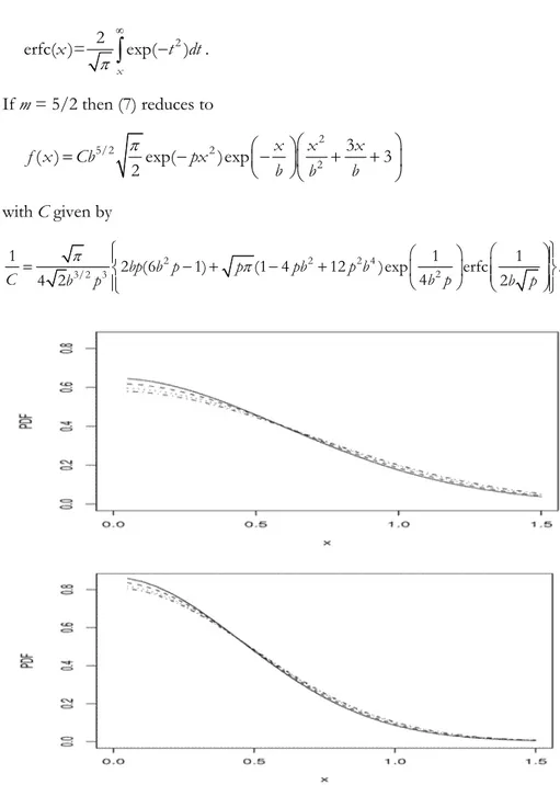
. If m = 5/2 then (7) reduces to 2 5/2 2 2 3 ( ) exp( )exp 3 2 x x x f x Cb px b b b π ⎛ ⎞⎛ ⎞ = − ⎜− ⎟⎜ + + ⎟ ⎝ ⎠⎝ ⎠ with C given by 2 2 2 4 2 3/2 3 1 2 (6 1) (1 4 12 )exp 1 erfc 1 . 4 4 2 bp b p p pb p b 2 C b p b p b p π π ⎧ ⎛ ⎞ ⎛ ⎞⎫ ⎪ ⎪ = ⎨ − + − + ⎜ ⎟ ⎜⎜ ⎟⎟⎬ ⎝ ⎠ ⎪ ⎝ ⎠⎪ ⎩ ⎭Figure 1 – Plots of the pdf (7) for b = 1, p = 1 and m = 1.5, 2, 3, 5 (top); and, b = 1, p = 2 and m = 1.5, 2, 3, 5 (bottom). The four curves in each plot are: the solid curve (m = 1.5), the curve of
lines (m = 2), the curve of dots (m = 3), and the curve of lines and dots (m = 5).
Figure 1 illustrates possible shapes of the pdf (7) for selected values of m and p. The four curves in each plot correspond to selected values of m. The effect of the parameters is evident.
3. MOMENTS
Suppose X is a random variable with pdf (7). If n is odd then it is obvious that ( n) 0
E X = . If n is even then one can write
2 0 ( n) 2 m nexp( ) m x E X C x px K dx b ∞ + ⎛ ⎞ = − ⎜ ⎟ ⎝ ⎠
∫
.By application of equation (2.16.8.4) in Prudnikov et al. (1986, volume 2), the above can be calculated as
( )/2, /2 ( )/2 2 2 1 1 1 1 ( ) exp 2 2 8 4 n m n m m n Cb n n E X m W p + Γ Γ b p − + b p ⎛ ⎞ ⎛ ⎞ + + ⎛ ⎞ ⎛ ⎞ = ⎜ + ⎟ ⎜ ⎟ ⎜ ⎟ ⎜ ⎟ ⎝ ⎠ ⎝ ⎠ ⎝ ⎠ ⎝ ⎠ (8)
where W denotes the Whittaker function defined by ( ) 1/2 1/2 1/2 , 0 exp( /2) exp( ) (1 ) ) ( 1/2) x x x Wλ ν xt t t dt µ µ λ µ λ µ λ ∞ + − − + − − = − + Γ − +
∫
.Using special properties of the Whittaker function, one can obtain the simpler form ( 1)/2 ( 1)/2 (( 1)/2) ( ( 1)/2) ( ) 2 (2 1)(1 ) n m m n m m n C n m n E X p + + b m n m + − Γ + Γ + + = + − − =1/(42) ( 1)/2 ( 1)/2 ) { exp( ( , )}z b p m n n d z z m z dz + − − Γ ⎛ ⎞ ×⎜ ⎟ ⎝ ⎠ , (9)
for half integer values of m. The expressions in (8) and (9) can be used to obtain Bayes estimators of the parameters of (6).
4. MAXIMUM LIKELIHOOD ESTIMATION
The highest posterior density set corresponding to (6) cannot be obtained in closed form. However, an approximation method is possible via a normal ap-proximation of the posterior density. The normal apap-proximation requires finding the maximum likelihood estimates of the parameters (b, p, m) in (7).
Suppose X1, X2,,..., Xn is a random sample from (7). Then the log likelihood
function for (b, p, m) is
2
1 1 1
log ( , , ) log n log| | n n log i
i i m i i i X L b p m n C m X p X K b = = = ⎛ ⎞ = + − + ⎜ ⎟ ⎝ ⎠
∑
∑
∑
.The derivatives with respect to the three parameters are: / 1 2 / 1 ( ) log ( ) b n i m i b i m i i X K X L n C mb b C b b K X X + = ∂ ∂ ∂ ∂ ⎧ ⎫ ⎪ ⎪ = + ⎨ − ⎬ ⎪ ⎪ ⎩ ⎭
∑
, (10) 2 1 log n i i L n C X p C p = ∂ ∂ ∂ = ∂ −∑
(11) and / / / 1 1 ( ) log log ( ) b m n n m i i b i i m i K X L n C X m C m K X ∂ = = ∂ ∂ ∂ ∂ = ∂ +∑
+∑
. (12)The partial derivatives in (10)-(12) can be computed by using the facts that 1 ( , )a z za exp( z) z − ∂Γ ∂ = − − , 2 2 2 ( ) ( ) , ( ) a ( , ; 1, 1;-z) , log ( ) ( ) a z a z F a a a a a z z a a a γ ψ ∂Γ Γ Γ ∂ = + + − + , and ( ) csc( ) [ 2cos( ) ( ) log { ( ) ( )} 2 2 K z z K z I z I z ν ν ν ν π πν πν ν − ∂ ∂ ⎛ ⎞ = − − ⎜ ⎟ + ⎝ ⎠ 2 2 0 ( 1) ( 1) ] ! ( 1) 2 ! ( 1) 2 k k K k z k z k k k k ν ν ψ ν ψ ν ν ν − + ∞ = Γ Γ ⎧ − + + + ⎫ ⎪ ⎛ ⎞ ⎛ ⎞ ⎪ + ⎨ − + ⎜ ⎟⎝ ⎠ + + + ⎜ ⎟⎝ ⎠ ⎬ ⎪ ⎪ ⎩ ⎭
∑
,where ψ(z)=∂logΓ(z)/∂z is the digamma function,
1 0 ( , ) exp( ) x a a x t t dt γ =
∫
− −is the incomplete gamma function, 1 2 1/2 1 ( ) (1 ) exp( ) 2 ( 1/2) m m m m x I x t xt dt m π − − Γ = − ± +
∫
( , ; , ; ) 0 ( ) ( ) 2 2F a b c d x ( ) ( ) k a k bk c k d k ∞ = =
∑
is the hypergeometric function, where (e)k = e(e + 1)" (e + k – 1) denotes the ascending factorial. The maximum likelihood estimators of (b,p,m) are the simultaneous solutions of the equations log /∂ L ∂b=0, log /∂ L ∂p= and 0
log /L m 0
∂ ∂ = .
5. APPLICATION
We use the data given by Section 5.7 of Chhikara and Folks (1989), reproduced in Table 1 below.
TABLE 1 Failure data of 23 ball bearings
17.88 28.92 33.00 41.52 42.12 45.60 48.48 51.84 51.96 54.12 55.56 67.80 68.64 68.64 68.88 84.12 93.12 98.64 105.12 105.84 127.92
128.04 173.40
The data consist of the number of million revolutions before failure for each of 23 ball bearings used in a life test. The background details about the data can be found in Lieblein and Zelen (1956). Chhikara and Folks (1989) showed by means of the Kolmogorov-Smirnov test that the inverse Gaussian distribution in (3) provides a good fit to the data in Table 1. If we assume that the parameters (λ,φ) have the prior given by (5) with n = 1/2, corresponding to unit standard de-viation, then the posterior for φ, the shape parameter, is
2 23 23 23/2 23/2 1 1 1 ( | ) exp 2 i i j j K x x φ π φ φ φ = = ⎛ ⎞ ⎛ ⎞ ∝ ⎜− ⎟ ⎜⎜ ⎟⎟ ⎝ ⎠ ⎝
∑ ∑
⎠ x .Using the results in Section 3, we obtain the Bayes estimate of φ as
2 23 23 25/2 23/2 1 1 0 2 23 23 23/2 23/2 1 1 0 1 exp 2 0.005788836 1 exp 2 i i j j i i j j K x d x K x d x φ φ φ φ φ φ φ φ ∞ = = ∞ = = ⎛ ⎞ ⎛ ⎞ − ⎜ ⎟ ⎜ ⎟ ⎜ ⎟ ⎝ ⎠ ⎝ ⎠ = ⎛ ⎞ ⎛ ⎞ − ⎜ ⎟ ⎜ ⎟ ⎜ ⎟ ⎝ ⎠ ⎝ ⎠
∑ ∑
∫
∑ ∑
∫
.This estimate suggests that the data are highly skewed. The earliest and the most popular model used to describe failure data is the exponential distribution. So, it is of interest to see whether the exponential model provides an adequate fit
for the data. Since the exponential and inverse Gaussian distributions are not nested, we test the adequacy by comparing the skewness values. It is known that the skewness for the two distributions are 2 and 3/ φ , respectively. So, testing for adequacy of the exponential model amounts to testing H0:φ=2.25 versus
1: 2.25
H φ≠ . Using the likelihood ratio, we obtain: 2{log (2.25| ) - log (0.006| }= 1505.880L L
− x x .
Since 2
1,0.95
1505.880 > 3.841=χ (we have assumed 2 1
χ distribution to be con-sistent with the classical likelihood inference although it may not hold exactly in the case of Bayesian inference), there is overwhelming evidence that the exponen-tial model cannot provide an adequate fit for the data. This is consistent with findings in Lieblein and Zelen (1956).
School of Mathematics SARALEES NADARAJAH
University of Manchester, UK
APPENDIX A: PARTICULAR FORMS OF Kν (x)
Note that 2 5/2 5/2 exp( )( 3 3) ( ) , 2 x x x K x x π − + + = 3/2 3/2 3 2 7/2 7/2 4 3 2 9/2 9/2 exp( )( 1) ( ) , 2 exp( )( 6 15 15) ( ) and 2 exp( )( 10 45 105 105) ( ) . 2 x x K x x x x x x K x x x x x x x K x x π π π − + = − + + + = − + + + + =
More generally, if ν − 1/2≥1 is an integer then
1/2 0 ( 1/2)!(2 ) ( ) exp( ) 2 . !( 1/2)! j j j x K x x x j j ν ν ν π ν − − ⎡ ⎤ ⎣ ⎦ = + − = − − −
∑
ACKNOWLEDGMENTSThe author would like to thank the Editor-in-Chief and the referee for carefully read-ing the paper and for their comments which greatly improved the paper.
REFERENCES
V. V. ANH, R. MCVINISH, C. PESEE, (2005), Estimation and simulation of the Riesz-Bessel distribution, “Communications in Statistics-Theory and Methods”, 34, pp. 1881-1897.
R. CHHIKARA, L. FOLKS, (1989), The Inverse Gaussian distribution: theory, methodology, and
applica-tions, Marcel Dekker, New York.
A.K. GUPTA, S. NADARAJAH, (2006), Beta Bessel distributions, “International Journal of Mathe-matics and Mathematical Sciences”, Article ID 16156.
B. HARRIS, A.P. SOMS, (1974), Properties of the generalized incomplete modified Bessel distributions with
applications to reliability theory, “Journal of the American Statistical Association”, 69, pp.
259-263.
P. KIELCZYNSKI, W. PAJEWSKI, (1993), Acoustic field of gaussian and Bessel transducers, “Journal of the Acoustical Society of America”, 94, pp. 1719-1721.
P. KIELCZYNSKI, W. PAJEWSKI, M. SZALEWSKI, (1993), Ultrasonic transducers with Bessel–function
dis-tribution of vibrational amplitude on their surfaces, “IEEE Transactions on Robotics and
Au-tomation”, 9, pp. 732-739.
J. LIEBLEIN, M. ZELEN, (1956), Statistical investigation of the fatigue life of deep-groove ball bearings, “Journal Research of the National Bureau of Standards”, 57, pp. 273-316.
F. MCNOLTY, (1967), Applications of Bessel function distributions, “Sankhyā”, B, 29, pp. 235-248. A.P. PRUDNIKOV, Y.A. BRYCHKOV, O.I. MARICHEV, (1986), Integrals and series, volumes 1, 2 and 3,
Gordon and Breach Science Publishers, Amsterdam.
N.A. SALINGAROS, (1991), Optimal current distribution for energy-storage in superconducting magnets, “Journal of Applied Physics”, 69, pp. 531-533.
V. SESHADRI, (1986), The Inverse Gaussian distribution: statistical theory and applications, Springer Verlag, New York.
H.M. SRIVASTAVA, S. NADARAJAH, (2006), Some families of Bessel distributions and their applications, “Integral Transforms and Special Functions”, 17, pp. 65-73.
L. THABANE, B.M.G. KIBRIA, (1999), On the generalized modified power Bessel distribution. “Journal of Statistical Research”, 33, pp. 9-22.
SUMMARY
A modified Bessel distribution of the second kind
Motivated by a Bayesian inference problem, a modification of the Bessel function dis-tribution is introduced. Various particular cases, expressions for its moments and estima-tion procedures are derived. An applicaestima-tion is illustrated to failure data.