UNIVERSITY
OF TRENTO
DIPARTIMENTO DI INGEGNERIA E SCIENZA DELL’INFORMAZIONE
38050 Povo – Trento (Italy), Via Sommarive 14 http://www.disi.unitn.it
OPERATORS FOR TRANSFORMING KERNELS
INTO QUASI-LOCAL KERNELS THAT IMPROVE SVM
ACCURACY
Nicola Segata and Enrico Blanzieri
July 2009
Technical Report # DISI-09-042
Operators for transforming kernels
into quasi-local kernels
that improve SVM accuracy
Nicola Segata and Enrico Blanzieri∗
June 24, 2009
Abstract
Motivated by the crucial role that locality plays in various learning approaches, we present, in the framework of kernel machines for classification, a novel family of operators on kernels able to integrate local information into any kernel obtaining quasi-local kernels. The quasi-local kernels maintain the possibly global properties of the input kernel and they increase the kernel value as the points get closer in the feature space of the input kernel, mixing the effect of the input kernel with a kernel which is local in the feature space of the input one. If applied on a local kernel the operators introduce an additional level of locality equivalent to use a local kernel with non-stationary kernel width. The operators accept two parameters that regulate the width of the exponential influence of points in the locality-dependent component and the balancing between the feature-space local component and the input kernel. We address the choice of these parameters with a data-dependent strategy. Experiments carried out with SVM applying the operators on traditional kernel functions on a total of 43 datasets with different characteristics and application domains, achieve very good results supported by statistical significance.
1
Introduction
Support Vector Machines [1] (SVM) are state-of-the-art classifiers and are now widely used and applied over a wide range of domains. Reasons for SVM’s success are multiple, including the presence of an elegant bound on generalization error [2], the fact that SVM is based on kernel functions k(·, ·) representing the scalar product of the sample mapped in a Hilbert space and the relative lightweight computational cost of the model in the evaluation phase. For a review on SVM and kernel methods the reader can refer to [3].
Locality in classification plays a crucial role [4]. In the framework of statistical learning theory, in fact, selecting the local influence of the training points used to classify a test point (i.e. the level of locality of the classifier), allows one to find a lower minimization of the guaranteed risk (i.e. a bound on the probability of classification error) with respect to “global” approaches as shown in [5]. Local learning algorithms [4, 6] are based on this theoretical consideration and they locally adjust the separating surface considering the characteristics of each region of the training set, the assumption being that the class of a test point can be more precisely determined by the local neighbors rather than by the whole training set especially for non-evenly distributed datasets. Notice that one of the most popular classification methods, ∗N. Segata and E. Blanzieri are with Department of Information and Telecommunication Technologies,
the K-Nearest Neighbors (KNN)1algorithm, is deeply based on the notion of locality. In kernel
methods, locality has been introduced with two meanings: i) as local relationship between the features, i.e. local feature dependence, adding prior information reflecting it, ii) as distance proximity between points, i.e. local points dependence, enhancing the kernel values for points that are close to each other and/or penalizing the points that are far from each other. The first meaning has been exploited by locality-improved kernels, the second by local kernels and local SVM.
Locality-improved kernels [3] take into account prior knowledge of the local structure in data such as local correlation between pixels in images. The way the prior information is integrated into the kernel depends on the specific task but, in general, the kernel increases similarity and correlation of selected features that are considered locally related. Locality-improved kernels were successfully applied on image processing [7] and on bioinformatics tasks [8] [9].
Local kernels are kernels such that, when the distance between a test point and a training point tends to infinity, the value of the kernel is constant and independent of the test point [10] [11]; if this condition is not respected the kernel is said to be global. A popular local kernel is the radial basis function (RBF) kernel that tends to zero for points whose distance is high with respect to a width parameter that regulates the degree of locality. On the other hand, distant points influence the value of global kernels (e.g. linear, polynomial and sigmoidal kernels). Local kernels and in particular the RBF kernel show very good classification capability but they can suffer from the curse of dimensionality problem [12] and they can fail with datasets that require non-linear long-range extrapolation. In this case, even if the tuning of the width parameter allows for the contribution of distant points, global kernel reflecting a particular conformation of the separating surface are generally preferred and permits better accuracies. An attempt to mix the good characteristics of local and global kernels is reported in [11] where RBF and polynomial kernels are considered for SVM regression.
Local SVM is a local learning algorithm and was independently proposed by Blanzieri and Melgani [13] [14] and by Zhang et al. [15] and applied respectively to remote sensing and visual recognition tasks. Other successful applications of the approach are detailed in [16] for general real datasets, in [17] for spam filtering and in [18] for noise reduction. The main idea of local SVM is to build at prediction time a sample-specific maximal marginal hyperplane based on the set of K-neighbors. In [13] it is also proved that the local SVM has chance to have a better bound on generalization with respect to SVM. However, local SVM suffers from the high computational cost of the testing phase that comprises for each sample the selection of the K nearest neighbors and the computation of the maximal separating hyperplane, and from the problem of tuning the K parameter. Although the first drawback prevents the scalability of the method for large datasets, some approximations of the approach have been proposed in order to improve the computational performances in [19] and [20]. In particular the approach we presented in [20] is asymptotically faster than SVM especially for non high-dimensional datasets basically maintaining the classification capabilities of KNNSVM, whereas the approach of [19] remains much slower than SVM and builds only local linear models.
Other ways of including locality in the learning process are based on the work of Amari and Wu [21] that modify the Riemannian geometry induced by the kernel in the input space intro-ducing a quasi-conformal transformation on the kernel metric with a positive scalar function. Particular choices of such scalar functions permitted in [21] to increasing the margin of the separating hyperplane through a two steps SVM training under the empirical assumption that the support vectors (detected with a primary SVM training) are located mainly in proximity of the hyperplane. In the bioinformatics field, a different particular choice of the scalar function 1From now on, for notational reasons, we refer to the K parameter of KNN based methods with upper-case
permitted to the authors of [22] to reach high accuracy in classification of tissue samples from their microarray gene expression levels through a KNN based scheme. Locality has been also used as the key factor to combine multiple kernel functions using a stationary (i.e. non-global) fashion as detailed in [23].
In this work we present a family of operators that transform an arbitrary input kernel into a kernel which has a component that is local and universal in the feature space of the input kernel. This resulting new family of kernels, opportunely tuned, maintains the original kernel behaviour for non-local regions, while increasing the values of the kernel for pairs of points that fall in a local region. In this way we aim to take advantage of both locality information and the long-range extrapolation ability of global kernels, alleviating also the curse of dimensionality problem of the local kernels and balancing the compromise between interpolation and generalization capability. The operators systematically map the input kernel functions into kernels that maintain the positive definite property and exploit the locality in the feature space which is a generalization of the standard locality meaning and it is central in the notion of quasi-local kernels. In such a way we are able to introduce the power of local learning techniques in the standard kernel methods framework modifying only the kernel functions and thus overcoming the computational limitation of the original formulation of local SVM. In particular, if the operators are applied on a local kernel, it turns out that the new kernel has a conceptually different meaning of locality, basically similar to a local kernel with variable kernel width. We give a practical way of estimating the optimal additional parameters introduced in the resulting kernel functions starting from the optimized input kernel and the penalty parameter of SVM.
Although we are focusing here on the classification task, our operators on kernels can be theoretically applied for every kernel-based technique in which locality plays a crucial role. It is the case of many kernel-based subspace analysis techniques like dimensionality reduction, manifold learning and feature selection techniques which are gaining importance in the last few years. Some of the most popular techniques are intrinsically based on locality such as Local Learning Embedding (LLE) [24] which has a kernel-based version [25] and it is equivalent to kernel principal component analysis (kernel PCA) [26] for a particular kernel choice and kernel Local Discriminant Embedding (kernel LDE) [27]. Other non naturally local techniques, have their local counterparts: Fisher Discriminative Analysis (FDA) [28] and its kernel-based version [29] with Local Fisher Discriminative Analysis (LFDA) [30], Generalized Discriminant Analysis (GDA) [31] with locally linear discriminant analysis (LLDA) [32]. Global techniques such as ISOMAP [33,34] can adopt their kernel version using a local kernel to include locality. Other approaches are based on developing and learning kernels subject to local constraints, as for example in [35]. An interesting discussion on local and global approaches for non-linear dimensionality reduction fall beyond the kernel methods field and it is addressed in [36].
The paper is organized as follows. After recalling in section 2 some preliminaries on SVM, kernel functions and local SVM, in section 3 we present the new family of operators that produces quasi-local kernels. The artificial example presented in section 4 illustrates intuitively how the quasi-local kernels work. In section 5 we propose a first experiment on 23 datasets with the double purpose of investigating the classification performance and of identifying the most suitable quasi-local operators. The most promising quasi-local kernels are applied in the experiment of section 6 to 20 large classification datasets. Finally, in section 7, we draw some conclusions.
2
SVM and kernel methods preliminaries
Support vector machines (SVMs) are classifiers with sound foundations in statistical learning theory [2]. The decision rule of an SVM is SVM(x) = sign(hw, Φ(x)iF + b) where Φ(x) :
Rp → F is a mapping in some transformed feature space F with inner product h·, ·i
F. The
parameters w ∈ F and b ∈ R are such that they minimize an upper bound on the expected risk while minimizing the empirical risk. The minimization of the complexity term is achieved by minimizing the quantity 1
2 · kwk2, which is equivalent to maximizing the margin between
the classes. The empirical risk term is controlled through the following set of constraints: yi(hw, Φ(xi)iF+ b) ≥ 1 − ξi with ξi ≥ 0 and i = 1, . . . , N (1) where yi ∈ {−1, +1} is the class label of the i-th nearest training sample. Such constraints
mean that all points need to be either on the borders of the maximum margin separating hyperplane or beyond them. The margin is required to be 1 by a normalization of distances. The presence of the slack variables ξi allows the search for a soft margin, i.e. a separation with
possibly some training set misclassification, necessary to handle noisy data and non-completely separable classes. By reformulating such an optimization problem with Lagrange multipliers αi (i = 1, . . . , N ), and introducing a positive definite kernel function k(·, ·) that substitutes
the scalar product in the feature space hΦ(xi), Φ(x)iF the decision rule can be expressed as:
SVM(x) = sign à N X i=1 αiyik(xi, x) + b !
where training points with nonzero Lagrange multipliers are called support vectors. The introduction of the positive definite (PD) kernels avoids the explicit definition of the feature space F and of the mapping Φ [3] [37], through the so-called kernel trick. A kernel is PD if it is the scalar product in some Hilbert space, i.e. the kernel matrix is symmetric and positive definite2.
The maximal separating hyperplane defined by SVM has been shown to have important generalization properties and nice bound on the VC dimension [2]. In particular we refer to the following theorem:
Theorem 1 (Vapnik [2] p.139). The expectation of the probability of test error for a maximal separating hyperplane is bounded by
EPerror ≤ E ½ min µ m l , 1 l · R2 ∆2 ¸ ,p l ¶¾
where l is the cardinality of the training set, m is the number of support vectors, R is the radius of the sphere containing all the samples, ∆ = 1/|w| is the margin, and p is the dimensionality of the input space.
Theorem 1 states that the maximal separating hyperplane can generalize well as the ex-pectation on the margin is large (since a large margin minimizes the ∆R22 ratio).
2.1 Local and global basic kernels
Kernel functions can be divided in two classes: local and global kernels [11]. Following [10] we define the locality of a kernel as:
Definition 1 (Local kernel). A PD kernel k is a local kernel if, considering a test point x and a training point xi, we have that
lim
kx−xik→∞
k(x, xi) → ci (2)
with ci constant and not depending on x. If a kernel is not local, it is considered to be global.
This definition captures the intuition that, in a local kernel, only the points that are enough close each other influences the kernel value. This does not directly implicate that the higher peak of the kernel value is in correspondence of points in the same position, although the most popular local kernel functions have this additional characteristic. In contrast, in a global kernel function, all the points are able to influence the kernel value regardless of their proximity.
In this work we will consider as baseline and as inputs of the operators we will introduce in the next section, the linear kernel klin, the polynomial kernel kpol, the radial basis function kernel krbf and the sigmoidal kernel ksig. We refer to these four kernels as reference input
kernels and we recall here their definitions:
klin(x, x0) = hx, x0i kpol(x, x0) = (γpol· hx, x0i + rpol)d
krbf(x, x0) = exp(−γrbf· ||x − x0||2) ksig(x, x0) = tanh(γsig· hx, x0i + rsig)
with γpol, γrbf, γsig > 0, rpol, rsig ≥ 0 and d ∈ N.
It is simple to show that, among the four input kernel listed above, the only local kernel is krbf since for kx − xik → ∞ we have that krbf(x, xi) → 0 (i.e. a constant that does not
depend on x), whereas klin, kpol and ksig are global.
For the radial basis function kernel krbf it is reasonable to set the parameter γrbf with the
inverse of the squared median of the of kxi− xjk, namely the Euclidean distances between
every pair of samples xi [38]. This because krbf(x, x0) can be written explicitly introducing
the kernel width as exp ³
−||x−x0||2
2·σrbf 2 ´
and in this way the distances are weighted with a value that is likely to be in same order of magnitude. More precisely, denoting with qh[kx − x0kZ]
the h percentile of the distribution of the distance in the Z space between every pair of points x, x0 in the training set, γrbf can be chosen as γrbf
h = 1/(2 · qh2[kx − x0kR
p
]). For h reasonable choices can be 10, 50 (i.e. the median) or 90 that should be in the same order of magnitude of the median, and 1 which enhances the local behaviour.
It is known that the linear, polynomial and radial basis function kernels are valid kernels since they are PD. It has been shown, however, that the sigmoidal kernel is not PD [3]; nevertheless it has been successfully applied in a wide range of domains as discussed in [39]. In [40] is showed that the sigmoidal kernel can be conditionally positive definite (CPD) for certain parameters and for specific inputs. Since CPD kernels can be safely used for SVM classification [41], the sigmoidal kernel is suitable for SVM only on a subset of the parameters and input space. In this work we use the sigmoidal kernel being aware of its theoretical limitations, which can be reflected in non-optimal solutions and convergence problems in the maximal margin optimization.
2.2 Local SVM
The method [13, 14] combines locality and searches for a large margin separating surface by partitioning the entire transformed feature space through an ensemble of local maximal margin hyperplanes. It can be seen as a modification of the SVM approach in order to obtain a local learning algorithm [4, 5] able to locally adjust the capacity of the training systems. The local learning approach is particularly effective for uneven distributions of training set samples in the input space. Although KNN is the simplest local learning algorithm, its decision rule
based on majority voting overlooks the geometric configuration of the neighbourhood. For this reason the adoption of a maximal margin principle for neighbourhood partitioning can result in a good compromise between capacity and number of training samples [42].
In order to classify a given point x0 of the p-dimensional input feature space, we need first
to find its K nearest neighbors in the transformed feature space F and, then, to search for an optimal separating hyperplane only over these K nearest neighbors. In practice, this means that an SVM classifier is built over the neighborhood of each test point x0. Accordingly, the
constraints in (1) become:
yrx(i)¡w · Φ(xrx(i)) + b¢≥ 1 − ξrx(i), with i = 1, . . . , K
where rx0 : {1, . . . , N } → {1, . . . , N } is a function that reorders the indexes of the N training points defined recursively as:
rx0(1) = argmin i=1,...,N kΦ(xi) − Φ(x0)k2 rx0(j) = argmin i=1,...,N kΦ(xi) − Φ(x0)k2 with i 6= rx0(1), . . . , rx0(j − 1) for j = 2, . . . , N In this way, xrx0(j) is the point of the set X in the j-th position in terms of distance from x0
and the following holds: j < K ⇒ kΦ(xrx0(j)) − Φ(x0)k ≤ kΦ(x
rx0(K)) − Φ(x
0)k because of the
monotonicity of the quadratic operator. The computation of the distance in F is expressed in terms of kernels as:
||Φ(x) − Φ(x0)||2= Φ2(x) + Φ2(x0) − 2hΦ(x), Φ(x0)i F =
= hΦ(x), Φ(x)iF + hΦ(x0), Φ(x0)iF− 2hΦ(x), Φ(x0)iF = k(x, x) + k(x0, x0) − 2k(x, x0). (3)
If the kernel is krbf or any polynomial kernels with degree 1, the ordering function is equivalent
to use the Euclidean metric. For non-linear kernels (other than krbf) the ordering function
can be different from that produced using the Euclidean metric. The decision rule associated with the method is:
KNNSVM(x) = sign à K
X
i=1
αrx(i)yrx(i)k(xrx(i), x) + b !
.
For K = N , the KNNSVM method is the usual SVM whereas, for K = 2, the method imple-mented with the linear kernel corresponds to the standard 1-NN classifier. Conventionally, in the following, we assume that also 1-NNSVM is equivalent to 1-NN.
The method can be seen as a KNN classifier implemented in the input or in a transformed feature space with a SVM decision rule or as a local SVM classifier. In this second case the bound on the expectation of the probability of test error becomes:
EPerror ≤ E ½ min µ m K, 1 K · R2 ∆2 ¸ , p K ¶¾
where m is the number of support vectors. Whereas the SVM has the same bound with K = N , apparently the three quantities increase due to K < N . However, in the case of KNNSVM the ratio R∆22 decreases because: 1) R (in the local case) is smaller than the radius of the sphere that contains all the training points; and 2) the margin ∆ increases or at least remains unchanged. The former point is easy to show, while the second point (limited to the case of linear separability) is stated in the following theorem [14].
Theorem 2. Given a set of N training points X = {xi ∈ Rp}, each associated with a label
yi ∈ {−1, 1}, over which is defined a maximal margin separating hyperplane with margin ∆X,
if for an arbitrary subset X0 ⊂ X there exists a maximal margin hyperplane with margin ∆X0 then the inequality ∆X0 ≥ ∆X holds.
Sketch of the proof. Observe that for X0 ⊂ X the convex hull of each class is contained in the
convex hull of the same class in X. Since the margin can be seen as the minimum distance between the convex hulls of different classes and since given two convex hulls H1, H2 the
minimum distance between them cannot be lower than the minimum distance between H0
1
and H2 with H0
1 ⊆ H1, we have the thesis. For an alternative and rigourous proof see [14].
As a consequence of Theorem 2 the KNNSVM has the potential of improving over both KNN and SVM as empirically shown in [13] for remote sensing, in [15] for visual applications, in [16] on 13 benchmark datasets, in [17] for spam filtering and in [18] for noise removal.
Apart from the SVM parameters (C and the kernel parameters), the only parameter of KNNSVM that needs to be tuned is the number of neighbors K. K can be estimated on the training set among a predefined series of natural numbers (usually a subset of the odd numbers between 1 and the total number of points) choosing the value that shows better predictive accuracy with a 10-fold cross validation approach. In this work, when we refer to the KNNSVM classifier we assume that K is estimated in this way.
3
Operators that transform kernels into quasi-local kernels
In this section we define the operators we use to integrate the locality information into existing kernels obtaining quasi-local kernels. We first introduce the framework of operators on kernel, then the quasi-local operators discussing their properties, definition, intuitive meaning and strategies to select their parameters.
3.1 Operators on kernels
An operator on kernels, generically denoted as O, is a function that accepts a kernel as input and transforms it into another kernel, i.e. O is an operator on kernels if O k is a kernel (supposing that k is a kernel). More formally:
Definition 2 (Operators on kernels). Denoting with lp a (possibly empty) list of parameters
that can be real constants and real-valued functions and with lk a (possibly empty) a-priori fixed-length list of PD kernels, Olp is an operator on kernels if k(x, x0) = (Olplk)(x, x0) with x, x0 ∈ X is positive definite for every choice of PD kernels in l
k.
An example of operator with an empty list of kernels that we can define is (Omulf )(x, x0) := f (x)f (x0) which is a PD kernel for every real-valued function f . Also the identity function can
be thought of as an operator on kernel such that (I k)(x, x0) = k(x, x0). Another example is the
exponentiation operator defined as (Oek)(x, x0) := exp(k(x, x0)). Although the focus in this work is on the class of operators for quasi local kernels, notice that, defining operators based on known properties of kernel, it is possible to prove the PD property of a kernel rewriting it starting from known PD kernels applying only operators on kernels.
3.2 Operators for quasi-local kernels
Our operators produce kernels that we call quasi-local kernels, combining the input kernel with another kernel based on the distance in the feature space of the input kernel. The formal definition of locality will be discussed in subsection 3.6 but basically the class of quasi-local kernels comprises those kernels that combine an input kernel with a kernel which is quasi-local in the feature space of the input kernel. In the case of a global kernel as input of the operators, the intuitive effect of the quasi-locality of the resulting kernels is that they are not local for definition 1 but at the same time the kernel score is significantly increased for samples that are
close in the feature space of the input kernel. In this way the kernel can take advantage from both the locality in the feature space and the long-range extrapolation ability of the global input kernel.
We first construct a kernel to capture the locality information of any kernel function; such a family of kernels takes inspiration from the RBF kernel, substituting the Euclidean distance with the distance in the feature space.
kexp(x, x0) = exp µ −||Φ(x) − Φ(x0)||2 σ ¶ σ > 0
where Φ is a mapping between the input space Rp and the feature space F. The feature space
distance ||Φ(x) − Φ(x0)||2 is dependent on the choice of kernel (see (3)):
||Φ(x) − Φ(x0)||2 = k(x, x) + k(x0, x0) − 2 · k(x, x0).
The kexp kernel can be obtained with the first operator, named Eσ, that accepts a positive
parameter σ applied on a kernel k producing Eσk = kexp. Explicitly, the Eσ operator is defined
as: (Eσk)(x, x0) = exp µ −k(x, x) − k(x0, x0) + 2k(x, x0) σ ¶ σ > 0. (4) Note that Eσklin= krbf so as a special case we have the RBF kernel. However, the kernels
obtained with Eσ consider only the distance in the feature space without including explicitly the input kernel. For this reason Eσk is not a quasi-local kernel.
In order to overcome the limitation of Eσ which completely drops the global information,
the idea is to weight the input kernel with the local information to obtain a real quasi-local kernel. So we include explicitly the input kernel in the output of the following operator:
(Pσk)(x, x0) = k(x, x0) · (Eσk)(x, x0) σ > 0. (5)
Observing that the Eσk kernel can assume values only between 0 and 1 (since it is an
expo-nential with negative exponent) and that the higher the distance in the feature space between samples the lower the value of the Eσk kernel, the idea of Pσ is to exponentially penalize the
basic kernel k with respect to the feature space distance between x and x0.
An opposite possibility is to amplify the values of input kernels in the cases in which the samples contain local information. This can be done simply by adding the Eσk kernel to the
input one.
(Sσk)(x, x0) = k(x, x0) + (Eσk)(x, x0) σ > 0. (6)
However, since Eσ gives kernels that can assume at most the value of 1 while the input kernel in
the general case does not have an upper bound, it is reasonable to weight the Eσ operator with a constant reflecting the order of magnitude of the values that the input kernel can assume in the training set. We call this parameter η and the new operator is:
(Sσ,ηk)(x, x0) = k(x, x0) + η · (Eσk)(x, x0) σ > 0, η ≥ 0. (7)
A different formulation of the Pσ operator that maintains the product form but adopts the
idea of amplifying the local information is: (PSσk)(x, x0) = k(x, x0)
£
1 + (Eσk)(x, x0)
¤
σ > 0, η ≥ 0. (8) Also in this case the parameter η that controls the weight of the Eσk kernel is introduced:
(PSσ,ηk)(x, x0) = k(x, x0)
£
1 + η · (Eσk)(x, x0)
¤
The quasi-local kernels produced by the operators defined in Eq. 5 6, 7, 8, 9 are more com-plicated then the corresponding input kernels, since it is necessary to evaluate k(x, x), k(x0, x0),
k(x, x0) and to perform a couple of addition/multiplication operation and an exponentiation
instead of the evaluation of k(x, x0) only. However, this is a constant computational overhead
in the kernel evaluation phase, that does not affect the complexity of the SVM algorithm either in the training or in the testing phase. Moreover, it is possible to implement a variant of the dot product that computes hx, xi, hx0, x0i, hx, x0i with only one traversing of x and x0
vectors, or precompute and store hx, xi for each sample in order to enhance the computational performances of the operators.
Intuitively all the kernels produces by Sσ, Sσ,η, PSσ and Sσ,η (Eq. 5 6, 7, 8, 9) are
quasi-local since they combine the original kernel with the quasi-locality information in its feature space. We will formalise this in subsection 3.6, while in the following subsection we will prove that the operators preserve the PD property of the input kernel.
3.3 The operators for quasi-local kernels preserve the PD property of the input kernels
We recall three well-known properties of PD kernels (for a comprehensive discussion of PD kernels refer to [3] or [37]):
Proposition 1 (Some properties of PD kernels).
(i) the class of PD kernels is a convex cone, i.e. if α1, α2 ≥ 0 and k1, k2 are PD kernels then
α1k1+ α2k2 is a PD kernel;
(ii) the class of PD kernels is closed under pointwise convergence, i.e. if k(x, x0) := limn→∞
kn(x, x0) exists for all x, x0, then k is a PD kernel;
(iii) the class of PD kernels is closed under pointwise product, i.e. if k1, k2 are PD kernels, then (k1k2)(x, x0) := k1(x, x0) · k2(x, x0) is a PD kernel.
The introduced operators preserve the PD property of the kernels on which they are applied, as stated in the following theorem.
Theorem 3. If k is a PD kernel, then O k with O ∈ {Eσ, Pσ, Sσ, Sσ,η, PSσ, PSσ,η} is a PD
kernel.
Proof. It is straightforward to see that, for a PD kernel k, all the kernels resulting from the introduced operators can be obtained using properties (i) and (iii) of Proposition 1, provided that Eσk is a PD kernel. So the only thing that remains to prove is that Eσk is PD.
Decom-posing the definition of (Eσk)(x, x0) into three exponential functions we obtain:
(Eσk)(x, x0) = exp ³ 2k(x,x0) σ ´ exp ³ −k(x,x) σ ´ exp ³ −k(x0,x0) σ ´
that can be written as:
(Eσk)(x, x0) = (Oe2k/σ)(x, x0) · f (x)f (x0)
where Oe2k/σ is the exponentiation of the 2k/σ kernel, and f is a real valued function such
that f (x) = exp(−k(x, x)/σ). The first term is the exponentiation of a kernel multiplied by a non-negative constant and, since the kernel exponentiation can be seen as the limit of the series expansion of the exponential function which is the infinite sum of polynomial kernels, for property (ii) we conclude that Oe2k/σ is a PD kernel. Moreover, recalling from the definition
of PD kernels, that the product f (x)f (x0) is a PD kernel for all the real-valued functions f defined in the input space [37] we conclude that Eσk is a PD kernel.
Obviously, if the input of Eσ is not a PD kernel, also the resulting function cannot be, in
the general case, a PD kernel since the exponentiation operator maintains the PD property only for PD kernels. So, in the case of the sigmoidal kernel as input kernel, the resulting kernel is still not ensured to be PD.
3.4 Properties of the operators
In order to understand how the operators modify the original feature space of the input kernel we study the distances in the feature space of the quasi-local kernels. The new feature space introduced by kernels produced by the operators is denoted with FO, the corresponding mapping function with ΦO and the distance between two input points mapped in FO with
distFO(x, x0) = m(ΦO(x), ΦO(x0)) where m is a metric in FO. Applying the kernel trick for distances, we can express the squared distances in FO as:
dist2
FO(x, x
0) = kΦ
O(x) − ΦO(x0)k2 = (O k)(x, x) + (O k)(x0, x0) − 2(O k)(x, x0). (10)
For O = Eσ, since it is clear that distF(x, x) = 0 for every x, we can derive distFEσ as follows:
dist2 FEσ(x, x 0) = exp³−dist2F(x,x) σ ´ + exp ³ −dist2F(x0,x0) σ ´ − 2 exp ³ −dist2F(x,x0) σ ´ = = 2 h 1 − exp ³ −dist2F(x,x0) σ ´i . (11)
Note that dist2
FEσ(x, x
0) ≤ 2 for every pair of samples, and so the distances in F
Eσ are bounded even if they are not bounded in F.
Substituting Pσ, Sσ,η and PSσ,η in Eq. 10, an taking into account Eq. 11, the distances in
FO for the quasi-local kernels are:
dist2 FPσ(x, x 0) = dist2 F(x, x0) + k(x, x0) dist2FEσ(x, x 0); dist2
FSσ,η(x, x0) = dist2F(x, x0) + η · dist2FEσ(x, x0);
dist2 FPSσ,η(x, x 0) = (1 + η) dist2 F(x, x0) + η · k(x, x0) dist2FEσ(x, x 0) = = dist2F(x, x0) + η · dist2F Pσ(x, x 0). (12)
We can notice that the distances in FEσ and in FSσ,η do not contain explicitly the kernel function but they are based only on the distances in F. So we can further analyse the behaviour of the distances in FEσ and FSσ,η with the following proposition.
Proposition 2. The operators Eσ and Sσ,η preserve the ordering on distances in F. Formally
distF(x, x0) < distF(x, x00) ⇒ distFO(x, x0) < distFO(x, x00) for O ∈ {Eσ, Sσ,η} and for every sample x, x0, x00.
Proof. It follows directly from the observations that distFEσ(x, x0) and distFSσ,η(x, x0) are
defined with strictly increasing monotonic functions, Eq. 11 and the second equation in Eq. 12 respectively, and that distF is always non-negative.
This means that Eσk kernel determines the same neighborhoods as k and that the Eσk exploits the locality information weighting the influence of the neighbors of a point in the feature space of k maintaining the property that points at distance d in the feature space of k influence the Eσk kernel score more than any other more distant points. In other words Eσk
modifies the influence of the points using the features space distances but the ordering on the weights is the same of the ordering on distances in the input space.
The Eσk kernel has also an interesting property regarding the class of universal kernels.
Roughly speaking, universal kernels, introduced in [43] and further discussed in [44–46], are kernels that permits to optimally approximate the Bayes decision rule or, equivalently, to learn an arbitrary continuous function uniformly on any compact subset of the input space. Applying Proposition 8 and Corollary 10 in [43], it turns out that Eσk is universal in the feature space of k. Intuitively this happens because Eσk builds an krbf kernel, which is universal, in the
feature space of k. This means that, regardless of the universality of the input kernel, the Eσ
always finds a space on which the resulting kernel is universal.
3.5 Connections between Eσ krbf and krbf with variable kernel width
Since krbf is a local kernel, a question that naturally arises concerns the behaviour of E σ krbf,
i.e. the quasi-local transformation of a local kernel. In particular the point is to understand if krbf and E
σ krbf exploit the same notion of locality. If it is the case, this would mean that
Eσ krbf and krbf are basically equivalent and identify the same features space, possibly under
certain parameter settings. This question is addressed by the following Proposition.
Proposition 3. There not exist two constant σ, γrbf ∈ R with σ > 0 and γ ≥ 0, such that,
for every x, x0 ∈ X with X with at least 3 distinct points, the following holds:
krbf(x, x0) = (Eσ krbf)(x, x0) (13)
Proof. Suppose, by contradiction, that there exist σ, γrbf ∈ R such that, for every x, x0 ∈ X,
Eq. 13 holds. It can be rewritten as:
exp(−γrbf · kx − x0k2) =
= exp µ
−exp(−γrbf · kx − xk2) + exp(−γrbf· kx0− x0k2) − 2 · exp(−γrbf· kx − x0k2) σ
Since exp(−γrbf · kx − xk2) = 1, we can obtain:
−γrbf· kx − x0k2 = −2 + 2 · exp(−γ
rbf· kx − x0k2)
σ ,
from which we have
exp(−γrbf· kx − x0k2) = 1 −γrbfσ
2 · kx − x
0k2
that can be written as:
krbf(x, x0) = 1 −γ
rbfσ
2 · kx − x
0k2.
Since, with respect to the square of the Euclidean distance kx−x0k2, krbf(x, x0) is a negative
exponential function, whereas 1 − kx − x0k2·γrbf2 σ is a non-increasing linear function, the two function can have no more than 2 points in common. Because σ and γrbf are constant, while
kx−x0k2 is not constant, it is straightforward to conclude that krbf(x, x0) 6= 1−kx−x0k2·γrbf2 σ at least for some x, x0 ∈ X. In this way we get a contradiction thus proving the proposition.
From this proposition we can conclude that Eσ krbf cannot be emulated by krbf and thus
it introduces an higher degree of locality. Intuitively an increased level of locality can be introduced locally adjusting the local parameters. In the specific case of krbf this intuition
can be applied permitting to the width parameter (1/γrbf) to be locally adaptive, as proposed
for example in [47]. The following proposition demonstrate that Eσ krbf is equivalent to krbf
Proposition 4. There exists a real-valued function f (σ, γrbf, kx − x0k) such that the following
holds for each x, x0 ∈ X:
exp µ − kx − x 0k2 f (σ, γrbf, kx − x0k) ¶ = (Eσ krbf)(x, x0) (14)
Proof. We can easily find such function f isolating it from Eq. 14: exp µ − kx − x0k2 f (σ, γrbf, kx − x0k) ¶ = exp µ −2 + 2 · exp(−γrbf· kx − x0k2) σ ¶ obtaining: f (σ, γrbf, kx − x0k) = σ 2 · kx − x0k2 1 − exp(−γrbf· kx − x0k2). (15)
We thus found the function regulating the variable krbf width. It can be shown that Eq. 15
has always positive derivative, meaning that it always grows as the distance between samples grows. This causes the kernel width to be lower for close points and higher for distant points, thus permitting to alleviate the tradeoff between over- and under-fitting on which a uniform kernel width is based. The variable kernel width is particularly crucial in presence of data with uneven densities.
-100 -50 0 50 100 -100 -50 0 50 100 (a) The whole two spiral dataset
-3 -2 -1 0 1 2 3 -3 -2 -1 0 1 2 3 (b) The two spiral dataset zoomed.
Figure 1: The behaviour of krbf (the dotted line) and E
σ krbf (the filled line) on the two
spiral problem (the samples of the two classes are denoted by + and ¯ symbols). The model parameters are obtained with 20-fold CV. The best training set accuracy is 0.823 for krbf and
0.907 for Eσkrbf.
We illustrate these considerations with the application of krbf and E
σ krbf on the two
spirals artificial dataset shown in Figure 1. Both krbf and Eσ krbf are applied with the best
best training accuracy of krbf is 0.823 whereas E
σ krbf reaches 0.907, meaning that the
quasi-local kernel approach is able to find a better decision function. This is evident also graphically, in fact, while in the peripheral regions of the datasets (see Figure 1(a)) both classifiers find a good decision function, whereas in the central region (see Figure 1(b)) krbf starts to clearly
underfit the data.
3.6 Quasi-local kernels
In this section, we formally introduce the notion of quasi-local kernels, and we show that kernels produced by the Sσ, Sσ,η, PSσ and Sσ,η are quasi-local kernels. Firstly, we introduce
the concept of locality with respect to a function:
Definition 3. Given a PD kernel k with implicit mapping function Φ : Rp 7→ F (namely
k(x, x0) = hΦ(x), Φ(x0)i), and a function Ψ : Rp 7→ F
Ψ, k is local with respect to Ψ if there
exists a function Ω : FΨ7→ F such that the following holds: 1. hΦ(x), Φ(xi)i = hΩ(Ψ(x)), Ω(Ψ(xi))i for all x, xi∈ Rp
2. lim
ku−vikFΨ→∞
hΩ(u), Ω(vi)i = ci with u = Ψ(x), vi = Ψ(xi) for some x, xi ∈ Rp and c i
constant and not depending on u.
In other terms, the notion of locality referred to samples in input space (Definition 1), is modified here in order to consider the locality in any space accessible from the input space through a corresponding mapping function. Notice that, as particular cases, we have that every local kernel is local with respect to the identity function and with respect to its own implicit mapping function.
With the next theorem we see that the Eσ formally respect the idea of producing kernels
that are local with respect to the feature space of the input kernel.
Theorem 4. If k is a PD kernel with the implicit mapping function Φ : Rp 7→ F, then E σk
is local with respect to Φ.
Proof. We have already shown that Eσk is a PD kernel given that k is a PD kernel (see
Theorem 3). It remains to show that Eσk is local with respect to Φ.
First we need to show that (Definition 3 point 1), denoted with Φ0 : Rp 7→ F0 the implicit
mapping function of Eσk, there exists a function Ω : F 7→ F0 such that Φ0(x) = Ω(Φ(x)).
Taking as Ω : F 7→ F0 the implicit mapping of the kernel exp³−ku−vik
σ ´ with u = Φ(x), vi = Φ(xi) with x, xi∈ Rp we have hΩ(u), Ω(vi)i = exp µ −ku − vik σ ¶ . (16)
Using the hypothesis on u and vi it becomes: exp µ −kΦ(x) − Φ(xi)k σ ¶ = hΩ(Φ(x)), Ω(Φ(xi))i. (17) The implicit mapping function of Eσk is Φ0 and so
hΦ0(x), Φ0(xi)i = (Eσk)(x, xi) (18) Moreover since (Eσk)(x, xi) = exp
³
−kΦ(x)−Φ(xi)k
σ
´
for definition of Eσ(see Eq. 4), substituting Eq. 17 into Eq. 18 we conclude that
Second, we need to show that (Definition 3 point 2) hΩ(u), Ω(vi)i → ci with ci constant
for kΩ(u) − Ω(vi)k → ∞. From the Eq. 16, it is clear that, as the distance between u = Φ(x) and vi= Φ(xi) tend to infinity, the kernel value is equal to the constant 0 regardless of x.
Now we can define the quasi-locality property of a kernel.
Definition 4 (Quasi-local kernel). A PD kernel k is a quasi-local kernel if k = f (kinp, kloc)
where kinp is a PD kernel with implicit mapping function Φ : Rp 7→ F, kloc is a PD kernel which is local with respect to Φ and f is a function involving legal and non trivial operations on PD kernels.
For legal operations on kernels we mean operations preserving the PD property. For non trivial operations we intend operations that always maintain the influence of all the input kernels in the output kernel; more precisely a function f (k1, k2) does not introduce trivial
operations if there exists two kernels k0 and k00 such that f (k0, k
2) 6= f (k1, k2) and f (k1, k00) 6=
f (k1, k2). Notice that the kinp kernel of the definition corresponds to the input kernel of the
operator that produces the quasi-local kernel k.
Theorem 5. If k is a PD kernel, then Sσk, Sσ,ηk, PSσk and Sσ,ηk are quasi-local kernels. Proof. Theorem 4 already states that Eσk is a PD kernel which is local with respect to the
implicit mapping function Φ of the kernel k which is PD for hypothesis. It is easy to see that all the kernels resulting from the introduced operators can be obtained using properties (i) and (iii) of Proposition 1 starting from the two PD kernels k and Eσk, and thus Sσk, Sσ,ηk,
PSσk and Sσ,ηk are PD kernels obtained with legal operations. Moreover, the properties (i) and (iii) of Proposition 1 introduce multiplications and sums between kernels and between kernels and constant. The sums introduced by the operators are always non trivial because they always consider positive addends, and so it is for the multiplications because they never consider null factors (the introduced constants are non null for definition).
Both quasi-local kernels and KNNSVM classifiers are based on the notion of locality in the feature space. However, two main theoretical differences can be found between them. The first is that in KNNSVM locality is included directly, considering only the points that are close to the testing point, while for the quasi-local kernels the information of the input kernel is balanced with the local information. The second consideration concerns the fact that KNNSVM has a variable but hard boundary between the local and non local points, while Sσ,η
and PSσ,η produce kernels whose locality decreases exponentially but in a continuous way. 3.7 Parameter choice and empirical risk minimization for quasi-local kernels There are two parameters for the operators on kernels through which we obtain the quasi-local kernels: σ, which is present in Eσand consequently in all the operators, and η, which is present
in Sσ,η and PSσ,η (Sσ and PSσ can be seen as special cases of Sσ,η and PSσ,η with η = 1).
The role of these two parameters will be better illustrated in the next section. Here we propose a strategy for choosing their values. The idea is that a quasi-local operator is applied on an already optimized kernel in order to further enhance the classification capability introducing locality. Notice that, in general, it would be possible to estimate the input kernel parameters, the SVM penalty parameter C and the operator parameters at the same time, but this is in contrast with the above idea. Ideally the operators can accept a kernel matrix without knowledge about the kernel function from which it is generated. So the approach we adopt here is to apply the operators on a kernel for which the parameters are already set, thus requiring only one parameter optimization (for Eσ, Pσ and PSσ) or two (for Sσ,η and PSσ,η).
0 1.5
0 1
y
x (a) klinand krbf
0 1.5 0 1 y x (b) Sσ,ηklinvarying η 0 1.5 0 1 y x (c) Sσ,ηklinvarying σ Figure 2: The separating hyperplanes for a two-feature hand-built artificial datasets defined by the application of the SVM (all with C = 3) with (a) linear kernel klin and RBF
ker-nel krbf (with γrbf = 150), (b) the S
σ,ηklin quasi-local kernel with fixed σ (σ = 1/150 =
1/γrbf) and variable η (η = 106, 50, 10, 1, 0.5, 0.1, 0.05, 0.03, 0.01, 0.005, 0.001, 0.000001),
and (c) the Sσ,ηklin quasi-local kernel with fixed η (η = 0.05) and variable σ (σ =
1/5000, 1/2000, 1/1000, 1/500, 1/300, 1/150, 1/100).
Moreover, we provide some data-dependent estimations of σ η permitting the reduction of the number of parameters values that need to be optimized (3 for η and 4 for σ).
The dataset-dependent estimation of σ take inspiration from the γrbf estimation, since
σ and γrbf play a similar role of controlling the width of the kernel. However, differently
from the krbf kernel, the E
σ operator uses distances in the feature space F (except for the
special case k = klin). More precisely, remembering that the data-dependent values of γrbf are
obtained with γhrbf = 1/(2 · q2
h[kx − x0kR
p
]) where qh[kx − x0kZ] denotes the h percentile of the
distribution of the distance in the Z space between every pair of points x, x0, the σ parameter can be estimated using σh= 2 · q2h[kx − x0kF] with h ∈ {1, 10, 50, 90} as for the γrbf case. For
η we adopt ηh= qh[kx − x0kF] with h ∈ {10, 50, 90}.
We thus have a total of 12 quasi-local parameter configurations, meaning that the model selection for quasi-local kernels in this scenario requires no more than 12 cross-validation runs to choose the best parameters. Notice that, comparing the cross-validation best values of the input kernel and quasi-local kernels, we implicitly test also the η = 0 case. Since Sσ,ηk and
PSσ,ηk with η = 0 are equivalent to k, Sσ,ηk and PSσ,ηk have the possibility to reduce to
k as a special case. In our empirical evaluation we will highlight the cases in which η = 0 is selected.
4
Intuitive behaviour of quasi-local kernels
The operators on kernels defined in the previous section aim to modify the behaviour of an input kernel k in order to produce a kernel more sensitive to local information in the feature space, maintaining however the original behaviour for regions in which the locality is not important. In addition the η and σ parameters control the balance between the input kernel k and its local reformulation Eσk, in other words the effects of the local information.
These intuitions are highlighted in Figure 2 with an example that illustrates the effects of the Sσ,η operator on the linear kernel klin using a two-feature hand-built artificial dataset.
Notice that this example is not limited to the combination of klinand krbf, because it represents
the intuition of what happens in the feature space of the original kernel applying the Sσ,η
operator. The transformed kernel is:
(Sσ,ηklin)(x, x0) = klin(x, x0) + η · (Eσklin)(x, x0) = klin(x, x0) + η · krbf(x, x0) (19)
with γrbf = 1/σ. So the S
σ,η operator on the klinkernel gives a linear combination of klinand
krbf. Figure 2(a) show the separate behaviours of the global term klin alone and of the local
term Eσklin= krbf alone. Figure 2(b) illustrates what happens when the local and the global
terms are combined with different values of η and a fixed σ. Figure 2(c) shows the behaviour of the separating hyperplane with a fixed balancing factor η but varying the σ parameter.
The η parameter regulates the influence on the separating hyperplane of the local term of the quasi-local kernel. In fact, in Figure 2(b), we see that all the planes lie between the input kernel (klin, obtained with η → 0 from S
σ,ηklin) and the local reformulation of the same kernel
(obtained with η = 106 from Sσ,ηklin which behaves as krbf since the high value of η partially
hides the effect of the global term). Moreover, since σ is low, the modifications induced by different values of η are global, influencing all the regions of the separating hyperplane.
We can observe in Figure 2(c), on the other hand, that σ regulates the magnitude of the distortion from the linear hyperplane for the region containing points close to the plane itself. The σ parameter in the Eσklin term of Sσ,ηklin has a similar role to the K parameter in the
local SVM approach (i.e. it regulates the range of the locality), even though K defines an hard boundary between local and non local points instead of a negative exponential one. It is important to emphasize that in the central region of the dataset the separating hyperplane remains linear, highlighting that the kernel resulting from the Sσ,η operator differs from the
input kernel only where the information is local.
The example simply illustrates the intuition behind the proposed family of quasi-local kernels, and in particular how the input kernel behaviour in the feature space is maintained for the regions in which the information is not local, so it is not important here to analyse the classification accuracy. However, kernels that are sensitive to important local information but retain properties of global input kernels, can also be obtained from very elaborated and well tuned kernels defined on high-dimensionality input spaces. In the following two sections we investigate the accuracy performances of the quasi-local kernels in a number of real datasets using a data-dependent method of choosing η and σ parameters.
5
Experiment 1
The goal of the first experiment is to compare the accuracy of SVM with quasi-local kernels against SVM with traditional kernels and kNNSVM. The evaluation is carried out on 23 non-large datasets.
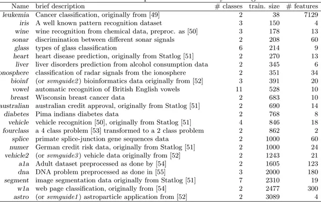
Table 1: The 23 datasets for Experiment 1 ordered by training set size.
Name brief description # classes train. size # features
leukemia Cancer classification, originally from [49] 2 38 7129
iris A well known pattern recognition dataset 3 150 4
wine wine recognition from chemical data, preproc. as [50] 3 178 13
sonar discrimination between different sonar signals 2 208 60
glass types of glass classification 6 214 9
heart heart disease prediction, originally from Statlog [51] 2 270 13
liver liver disorders prediction from alcohol consumption data 2 345 6
ionosphere classification of radar signals from the ionosphere 2 351 34
bioinf (or svmguide2 ) bioinformatics data originally from [52] 3 391 20
vowel automatic recognition of British English vowels 11 528 10
breast Wisconsin breast cancer data 2 683 10
australian australian credit approval, originally from Statlog [51] 2 690 14
diabetes Pima indians diabetes data 2 768 8
vehicle vehicle recognition [50], originally from Statlog [51] 4 846 18
fourclass a 4 class problem [53] transformed to a 2 class problem 2 862 2
splice primate splice-junction gene sequences data 2 1000 60
numer German credit risk data, originally from Statlog [51] 2 1000 24
vehicle2 (or svmguide3 ) vehicle data originally from [52] 2 1243 21
a1a Adult dataset preprocessed as done by [54] 2 1605 123
dna DNA problem preprocessed as done in [55] 3 2000 180
segment image segmentation data originally from Statlog [51] 7 2310 19
w1a web page classification, originally from [54] 2 2477 300
astro (or svmguide1 ) astroparticle application from [52] 2 3089 4
5.1 Experimental procedure
Table 1 lists the 23 datasets from different sources and scientific fields used in this experiment; we took all the freely available datasets from the LibSVM repository [48] with training set with no more than 3500 samples. Some datasets are multiclass and the number of features ranges from 2 to 7129.
The reference input kernels for the quasi-local operators considered are the linear kernel klin, the polynomial kernel kpol, the radial basis function kernel krbf and the sigmoidal kernel
ksig. The quasi-local kernels we tested are those resulting from the application of the E σ, Pσ,
Sσ,η, PSσ,η operators on the reference input kernels. We also evaluated the accuracy of the KNNSVM classifier with the same reference input kernels.
The methods are evaluated using 10-fold cross validation. The assessment of statistical significant difference between two methods on the same dataset is performed with the two-tailed paired t-test (α = 0.05) on the two sets of fold accuracies. Although the count of positive and negative significative difference can be used to establish if a method performs better than another on multiple datasets, it has been shown [56] that the Wilcoxon signed-ranks test [57] is a theoretically safer (with respect to parametric tests it does not assume “normal distributions or homogeneity of variance” ) and empirically stronger test. For this reason the final assessment of statistical significance difference on the 23 datasets is performed with the Wilcoxon signed-ranks test (in case of ties, the rank is calculated as the average rank between them).
The model selection is performed on each fold with a inner 5-fold cross validation as follows. For all the methods tested, the regularization parameter C is chosen in {2−5, 2−4, . . . , 29, 210}. For the polynomial kernel we adopt the widely used homogeneous polynomial kernel (γpol = 1,
rpol = 0), selecting a degree non higher than 5. The choice of γrbf for the RBF kernel is
done adopting γhrbf where h is chosen among {1, 10, 50, 90ua} as described in 2.1. For the sigmoidal kernel, rsig is set to 0, whereas γsig is chosen among {2−7, 2−6, . . . , 2−1, 20}. For the
above for each input kernel, whereas σ is chosen using σF
h with h ∈ {1, 10, 50, 90} and η
using ηF
.h with h ∈ {10, 50, 90} and (implicitly) η = 0 as described in Section 3.7 through
a 5-fold cross validation on the same folds used for model selection on the input kernels. Finally, the value of K for KNNSVM is automatically chosen on the training set between K = {1, 3, 5, 7, 9, 11, 15, 23, 39, 71, 135, 263, 519, 1031} (the first 5 odd natural numbers followed by the ones obtained with a base-2 exponential increment from 9) as described in section 2.2. We used LibSVM library [48] version 2.84 for SVM training and testing, extending it with a object-oriented architecture for kernel calculation and specification. For the quasi-local kernels we store the values of hx, xi for each sample in order to obtain the quasi-quasi-local kernel value computing only one scalar product, i.e. hx, x0i, instead of three. The KNNSVM
implementation is based on the same version of LibSVM. The experiments are carried out on multiple Intel°R XeonTMCPU 3.20GHz systems, setting the kernel cache dimension to 1024Mb and interrupting the experiments that are not terminated after 72 hours.
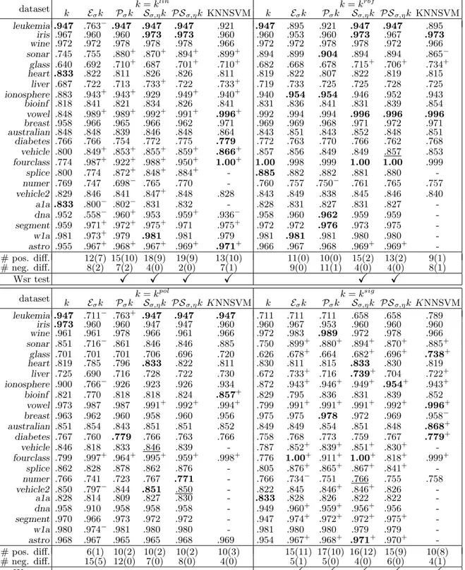
5.2 Results
Table 2 reports the 10-fold cross validation accuracy of SVM with the four considered input kernels, SVM with the quasi-local kernels obtained applying the Eσ, Pσ, Sσ,η, PSσ,η operators
and KNNSVM. Some KNNSVM results are missing due to the computational effort of the method, corresponding to the cases in which KNNSVM does not terminates within 72 hours. The + and − denotes quasi-local kernel and KNNSVM results that are significatively better
(and worse) than the corresponding input kernels according to the two-tailed paired t-test (α = 0.05). The total number of datasets in which quasi-local kernels and KNNSVM perform better (and worse) than the corresponding input kernels are reported, with the number of significative differences in parenthesis. The last row reports the Wilcoxon signed-ranks tests to assess the significant improvements of quasi-local kernels over corresponding input kernels on all the datasets (for KNNSVM only on the datasets for which the results are present). The cases in which, for Sσ,η, PSσ,η, the model selection chose η = 0 for all the 10 folds thus giving
the same results of the input kernels, are underlined. In bold, are highlighted the best 10-fold cross validation accuracy achieved for a specific dataset among all the methods and kernels. 5.3 Discussion
The KNNSVM results basically confirm the earlier assessment [16], although the model selec-tion is performed here differently; KNNSVM is able to improve, according to the Wilcoxon signed-rank test, the classification generalization accuracy of SVM with the klinkernel (10
two-tailed paired t-test significant improvements, 1 deteriorations) and ksig kernel (8 two-tailed paired t-test significant improvements, 1 deteriorations). Instead we do not have evidence of improved generalization accuracy on the benchmark datasets for the kpol kernel and krbf
kernel, although we showed in [16] that, for krbf, there are scenarios in which KNNSVM can be particularly indicated.
Eσk seems to perform significantly better than k for ksig and for klin (although without
statistical evidence), whereas there are no overall improvement for krbf, and for kpol the accuracies are deteriorated. These results are probably due to the choice of not re-performing model selection for Eσk in particular for the C parameter. In fact Eσ is the only operator
that does not contain the input kernel explicitly in the resulting one, and thus the optimal parameters can be very different. This is confirmed by the fact that Eσklin is equivalent to
krbf but their results, as reported in Table 2, appears to be are very different.
The results of Pσk are slightly better than Eσk. According to the Wilcoxon signed-rank test, it is better than k for k = ksig and k = krbf, but not for krbf and kpol. In total, the