Dottorato di Ricerca
in
“Ricerca Operativa” (MAT/09)
XX ciclo
Tesi di Dottorato
Topics in real-time fleet
management
Emanuele Manni
Supervisori Coordinatore del corso di dottorato
prof. Gianpaolo Ghiani prof. Lucio Grandinetti
UNIVERSITY OF CALABRIA
PhD
in
“Operations Research” (MAT/09)
cycle XX
PhD Thesis
Topics in real-time fleet
management
Emanuele Manni
Advisors PhD Coordinator
prof. Gianpaolo Ghiani prof. Lucio Grandinetti
Summary
The field of real-time fleet management has considerably grown during the last years, mainly due to recent developments in the economic and technologic sectors, allowing companies to focus on aspects not considered before, in order to be competitive on the market. Given these aspects, developing systems whereby goods are delivered to customers on time becomes crucial. Under this setting the key aspect is the avail-ability of real-time information, like, for instance, vehicles location, road congestion, current fleet status, etc. For this purpose, advances in information technology and telecommunications, together with continually growing amount of data, offer oppor-tunities for transportation companies to obtain this information with a relatively low effort. One of the most important tools available to companies is the ability to equip drivers with modern tools such as Global Positioning System (GPS) devices, eventually embedded into palmtop computers, in order to exactly know where the vehicles are and also to provide the drivers real-time directions.
In this thesis various issues concerning real-time fleet management are studied. The conventional vehicle routing problem (VRP) consists of determining a set of vehicle routes so that each customer of a set is visited exactly once and the total cost is minimized. Although dynamic VRPs represent important applications in many distribution systems, past research has focused mainly on static aspects of the VRPs. However, in the recent years, because of the rapid development in the telecommunications and computer hardware sectors, together with an increased fo-cus on just-in-time logistics, a lot of efforts are being devoted to research on the more complex dynamic version of the VRP. The thesis begins by introducing the static VRP along with its dynamic counterpart (DVRP) and gives a discussion of the differences between the conventional static VRP and the dynamic VRP. Next, the main features of real-time vehicle routing problems are illustrated and a survey of the existing literature dealing with the dynamic vehicle routing problem as well
optimal policy through a Markov decision process is proposed as well as lower and upper bounds on the optimal policy cost are developed.
Then, an interesting question to answer in dynamic routing is whether or not it is worthwhile using complex procedures in order to design a priori routes. For this purpose, we consider several approaches for determining the a priori route for our dynamic routing problem and we determine under which circumstances the use of a priori routing can offer some value.
Next, we present the Dynamic and Stochastic Vehicle Dispatching Problem with Pickups and Deliveries, a real-time problem faced by local area (e.g., intra-city) courier companies serving same-day pickup and delivery requests for the transport of letters and small parcels. We develop anticipatory algorithms that evaluate al-ternative solutions through a short-term demand sampling and a fully sequential procedure for indifference zone selection.
Moreover, we introduce the same-day Courier Shift Scheduling Problem, a tac-tical problem faced by same-day courier companies, which amounts to minimize the staffing cost subject to probabilistic service level requirements.
Finally, we give our conclusions, as well as provide some directions for further research on real-time VRPs.
Riassunto (In Italian)
Il settore della gestione di flotte in tempo reale ha visto un crescente aumento di interesse nel corso degli ultimi anni, principalmente grazie ai recenti sviluppi di natura tecnologica ed economica, che hanno consentito alle aziende del settore di spostare il proprio focus su aspetti fino a quel momento trascurati, con l’obiettivo di acquisire una maggiore competitivit`a sul mercato. A questo proposito, un aspetto di cruciale importanza `e la progettazione e lo sviluppo di sistemi di gestione di flotte in tempo reale in cui i beni sono consegnati ai clienti secondo modalit`a e tempi da loro richiesti. In questo contesto, un ruolo chiave `e rappresentato dalla disponibilit in tempo reale di informazioni, quali, ad esempio, la posizione dei veicoli, la situazione di congestione stradale o lo stato corrente della flotta di veicoli. In questo senso, i grandi progressi effettuati nella tecnologia dell’informazione e delle telecomunicazioni, insieme alla sempre maggiore disponibilit`a di dati storici, offrono la possibilit`a alle aziende di trasporti di ottenere le informazioni volute con uno sforzo relativamente basso. Uno degli strumenti pi`u importanti a disposizione delle aziende la possibilit`a di fornire ai dipendenti dispositivi moderni quali, ad esempio, i GPS, eventualmente integrati in dispositivi palmari, con l’obiettivo di conoscere in ogni istante la posizione dei veicoli e di fornire indicazioni in tempo reale.
Obiettivo della presente tesi `e analizzare diversi aspetti legati alla gestione di flotte in tempo reale. Il classico problema di instradamento dei veicoli (VRP) con-siste nel determinare un insieme di rotte in modo tale che il costo complessivo sia minimizzato e che ciascun cliente sia visitato esattamente una volta. Bench´e il VRP abbia applicazioni importanti in una grande variet`a di contesti di logistica distribu-tiva, buona parte degli sforzi di ricerca degli ultimi decenni `e stata indirizzata allo studio della versione statica del VRP. Occorre dire, comunque, che, nel corso degli ultimi anni, il crescente interesse nella logistica just-in-time e il rapido sviluppo tec-nologico, hanno contribuito ad incrementare l’interesse nei confronti della versione
zano le differenze principali tra queste due varianti del problema. In seguito viene presentata una rassegna della letteratura esistente relativa a questa classe di prob-lemi, con una particolare enfasi sul problema della determinazione di rotte a priori e sull’ottimizzazione in tempo reale.
Successivamente si introduce il problema del commesso viaggiatore dinamico e stocastico (Dynamic and Stochastic Traveling Salesman Problem) e, per mezzo di un processo decisionale markoviano, si individua una politica ottimale, oltre a fornire dei limiti inferiore e superiore al costo di tale politica.
Nel seguito si prova a rispondere ad un quesito molto attuale nei problemi di-namici di instradamento dei veicoli, relativo alla possibilit`a di utilizzare procedure pi`u o meno complesse per la determinazione di rotte a priori per i veicoli. A tale scopo, vengono considerate diverse strategie a priori e si individuano le strategie che offrono le migliori prestazioni con riferimento al particolare problema di routing analizzato.
Nella sezione successiva si introduce il problema di assegnamento di richieste ai veicoli dinamico e stocastico con prelievo e consegna (Dynamic and Stochastic Vehicle Dispatching Problem with Pickups and Deliveries). Tale problema `e af-frontato in tempo reale dalle aziende di corrieri urbani che forniscono un servizio di prelievo e consegna di lettere o piccoli imballaggi nel corso della stessa giornata. Relativamente a tale problema, sono proposti degli algoritmi anticipativi che valu-tano diverse soluzioni alternative tramite un campionamento a breve termine della domanda futura ed una procedura completamente sequenziale per la selezione della zona di indifferenza.
In aggiunta, si introduce il problema di schedulazione dei turni per un’azienda di corrieri urbani (Same-day Courier Shift Scheduling Problem), un problema di natura tattica per questo tipo di aziende, che consiste nel minimizzare i costi del personale, dovendo rispettare dei vincoli di natura probabilistica sulla qualit`a del servizio.
Infine, si riportano le conclusioni e si individuano le possibile direzioni di ricerca futura.
Acknowledgments
First of all, I am deeply indebted to my advisors, Prof. Gianpaolo Ghiani and Prof. Barrett Thomas. To each of them I owe a great debt of gratitude for their patience, inspiration and friendship. Thank you Gianpaolo for proposing me a promising research subject and motivating me to work on challenging problems. You came down to my level in order to collaborate with me, you was a real partner, before being a master. Thank you Barry for all the guiding, cooperation, encouragements, lasting support, and for making me feel like at home when I visited you at the University of Iowa.
Next, I would like to thank all the colleagues at the Logistics Lab, especially Adriana, Marco and Matteo, for being real friends more than colleagues. We spent many enjoyable hours together.
Thanks also to my family who have been extremely understanding and support-ing. They sustained me both in my studies and life with their love and their presence and put an immense trust in me. Thanks for everything. A particular thanks goes to my brother Andrea for sharing with me these last three years as PhD students.
Finally, last but certainly not least I wish to thank Alessandra for all her love, support and comprehension throughout all these years. Thanks for encouraging me with the right words when I needed them, thanks for being there when I needed you.
Emanuele Manni November 2007
Summary II
Riassunto (In Italian) IV
Acknowledgments VI
1 Introduction 1
1.1 Outline of the thesis . . . 3
1.2 Static vs Dynamic Vehicle Routing Problems . . . 4
1.3 Characterization of Dynamic Vehicle Routing Problems . . . 6
1.3.1 The degree of dynamism of a problem . . . 6
1.3.2 Objectives . . . 7
1.3.3 Spatial distribution and time pattern of user requests . . . 7
1.3.4 Comparing different dispatching and routing procedures . . . 8
1.4 Literature review . . . 8
1.4.1 A Priori Optimization Based Methods . . . 9
1.4.2 Real-time Optimization Methods . . . 11
2 The Dynamic and Stochastic TSP 14 2.1 Introduction . . . 14
2.2 A lower bound on the optimal policy expected penalty . . . 15
2.3 Heuristic policies . . . 16
2.4 A Markov Decision Process . . . 17
2.5 A numerical example . . . 20
2.6 Computational Results . . . 24
3.1 Introduction . . . 27
3.2 Model Formulation . . . 29
3.3 Preliminary Results and Optimality Equations . . . 32
3.4 A priori route design . . . 33
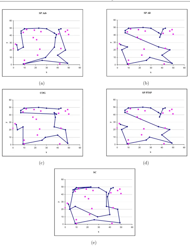
3.4.1 Heuristic 1: Shortest Path through Advance-Request Cus-tomers (SP Adv) . . . 33
3.4.2 Heuristic 2: Shortest Path through both Advance- and Late-Request Customers (SP All) . . . 33
3.4.3 Heuristic 3: Center-of-Gravity Procedure (COG) . . . 34
3.4.4 Heuristic 4: Probabilistic Traveling Salesman Problem Short-est Path (SP PTSP) . . . 35
3.4.5 Heuristic 5: A Priori Routing with Sampling and Consensus (SC) . . . 35
3.5 Empirical Results . . . 39
3.5.1 Implementation and Data Set Generation . . . 39
3.5.2 Results . . . 40
3.6 Conclusions . . . 43
4 The Dynamic and Stochastic VDPPD 51 4.1 Introduction . . . 51
4.2 Problem Statement . . . 52
4.3 The anticipatory algorithms . . . 53
4.3.1 Approximation of the near-future inconvenience . . . 54
4.3.2 Determination of the number of samples . . . 54
4.3.3 Generation of alternative solutions . . . 57
4.3.4 Anticipatory local search . . . 57
4.4 Experimental Results . . . 58
4.5 Conclusions . . . 62
5 The SSP in the Same-day Courier Industry 67 5.1 Introduction . . . 67
5.2 Problem Formulation . . . 69
5.4 Computational Results . . . 77 5.4.1 Careless GRASP . . . 79 5.4.2 Careful GRASP . . . 79 5.4.3 ANE GRASP . . . 79 5.4.4 Results . . . 80 5.5 Conclusions . . . 81
6 Conclusions and Future Work 87 6.1 Conclusions . . . 87
6.2 Future work . . . 89
List of publications 90
Chapter 1
Introduction
Gutta cavat lapidem; non vi, sed saepe cadendo. Huic addiscit homo: non vi, sed saepe legendo. Anonymous
Vehicle Routing Problems (VRPs) are central to logistics management both in the
private and public sectors. They consist of determining optimal vehicle routes through a set of users, subject to side constraints. The most common operational constraints impose that the total demand carried by a vehicle at any time does not exceed a given capacity, the total duration of any route is not greater than a prescribed bound, and service time windows set by customers are respected. In long-haul routing, vehicles are typically assigned one task at a time while in short-long-haul routing, tasks are of short duration (much shorter than a work shift) and a tour is to be built through a sequence of tasks. For a survey on the most relevant modeling and algorithmic issues on VRPs, see the recent book by Toth and Vigo (2002).
There exist several important problems that must be solved in real time. In what follows, we review the main applications that motivate the research in the field of the real-time VRPs.
Dynamic fleet management. Several large scale trucking operations require real-time dispatching of vehicles for the purpose of collecting or delivering shipments. Im-portant savings can be achieved by optimizing these operations (Brown and Graves,
1981, Brown et al., 1987, Powell, 1986, 1990, Goetschalckx, 1988, Rego and Rou-cairol, 1995, Savelsbergh and Sol, 1998).
Vendor-managed distribution systems. In vendor-managed systems, distri-bution companies estimate customer inventory level as to replenish the customers before they run out of stock. Hence, demands are known beforehand in principle and all customers are static. However, because demand has always a random com-ponent, some customers (usually a small percentage) may run out of stock and have to be serviced urgently (Campbell et al., 1998, Larsen, 2000).
Couriers. Long-distance couriers need to collect locally outbound parcels before sending them to a remote terminal to consolidate loads. Also, loads coming from remote terminals have to be distributed locally. Most pick-up requests are dynamic and have to be serviced the same day if possible (Gendreau et al., 1999, 2006, Cordeau et al., 2002).
Rescue and repair service companies. There are several companies providing rescue or repair services (broken car rescue, appliance repair, etc.) (Madsen et al., 1995b, Weintraub et al., 1999, Brotcorne et al., 2003).
Dial-A-Ride Systems. Dial-a-ride systems provide transportation services to peo-ple between given origin-destination pairs. Customers can book a trip one day in advance (static customers) (Cordeau and Laporte, 2003) or make a request at short notice (dynamic customers) (Roy et al., 1984, Madsen et al., 1995a).
Emergency Services. Emergency services comprise police, fire fighting and am-bulance services. By definition, all customers are dynamic. Moreover, the demand rate is usually low so that vehicles become idle from time to time. In this context, relocating idle vehicles in order to anticipate future demands or to escape from down-town rush hour traffic jam is an important consideration (Psaraftis, 1980, Gendreau et al., 1997, 2001).
Taxi Cab Services. In taxi cab services, almost every customer is dynamic. As in emergency services, relocating temporary idle vehicles is a consideration.
Due to recent advances in information and communication technologies, vehicle fleets can now be managed in real-time. When jointly used, devices like Geographic Information Systems (GIS), Global Positioning Systems (GPS), traffic flow sensors, and cellular telephones are able to provide relevant real-time data, such as current vehicle locations, new customer requests and periodic estimates of road travel times (Brotcorne et al., 2003). If suitably processed, this large amount of data can be
used to reduce cost and improve service level. To this end, revised routes have to be generated as soon as new events occur.
In recent years, three main developments have contributed to the acceleration and quality of algorithms relevant in a real-time context. The first is the increase in computing power due to better hardware. The second is the development of powerful metaheuristics whose main impact has been mostly on solution accuracy even if this gain has sometimes been achieved at the expense of computing time. The third development has arisen in the field of parallel computing. The combination of these three features has yielded a new generation of powerful algorithms that can effectively be used to provide real-time solutions in dynamic contexts.
1.1
Outline of the thesis
This thesis discusses various issues concerning real-time fleet management. In the present chapter, we introduce the vehicle routing problem (VRP) along with its dynamic counterpart (DVRP), and we give a discussion of the differences between the conventional static VRP and the dynamic VRP. Next, we illustrate the main features of real-time vehicle routing problems. Moreover, we present the notion of degree of dynamism, first introduced by Lund et al. (1996) and then extended by Larsen (2000). We list the different objectives that are to be achieved in dynamic problems. In addition, we present the different hypothesis on the spacial distribution of demands together with different possibilities for comparing routing and dispatch-ing policies. The chapter closes with a survey of the existdispatch-ing literature dealdispatch-ing with dynamic routing problems. The emphasis of the section is on both a priori and real-time optimization methods.
In chapter 2, we introduce the Dynamic and Stochastic Traveling Salesman Prob-lem and propose an optimal policy through a Markov Decision Process as well as develop lower and upper bounds on the optimal policy cost.
In chapter 3, we present several strategies for implementing a priori routes within a dynamic routing context, and we identify situations in which the use of more involved a priori strategies can give some benefit.
In chapter 4, we consider the Dynamic and Stochastic Vehicle Dispatching Prob-lem with Pickups and Deliveries, a real-time probProb-lem faced by local area (e.g., intra-city) courier companies serving same-day pickup and delivery requests for the
transport of letters and small parcels. We develop anticipatory algorithms that evaluate alternative solutions through a short-term demand sampling and a fully sequential procedure for indifference zone selection. A peculiar feature of this pro-cedures is that they allow the elimination, at an early stage of experimentation, those solutions that are clearly inferior, thus reducing the overall effort to select the best.
In chapter 5, we consider the same-day Courier Shift Scheduling Problem, a tactical problem faced by same-day courier companies, which amounts to minimizing the staffing cost subject to probabilistic service level requirements.
Then, in chapter 6, we give our conclusions in a brief summary of the discussions of this thesis as well as provide some directions for further research on real-time VRPs.
1.2
Static vs Dynamic Vehicle Routing Problems
A vehicle routing problem is said to be static if its input data (for example, travel times and demands) do not depend explicitly on time, otherwise it is dynamic. Moreover, a VRP is deterministic if all input data are known when designing vehicle routes, otherwise it is stochastic.
Static VRPs. A static problem can be either deterministic or stochastic. In deterministic and static VRPs (like the classical Capacitated VRP surveyed in Toth and Vigo (2002)) all data are known in advance and time is not taken into account explicitly. In stochastic and static VRPs (Laporte and Louveaux, 1998), vehicle routes are designed at the beginning of the planning horizon, before uncertain data become known. Uncertainty may affect which service requests are present, user demands, user service times or travel times. If input data are uncertain, it is usually impossible to satisfy the constraints for all realizations of the random variables. If uncertainty affects the constraints but the objective function is deterministic, it can be required that constraints be satisfied with a given probability (Chance
Constrained Programming, CCP). In a more general approach, a first phase solution
is constructed before uncertain data are available and corrective (or recourse) actions are taken at a second stage once all the realisations of the random variables become known. The objective to be minimized is the first stage cost plus the expected recourse cost (Stochastic Programming with Recourse, SPR).
Dynamic VRPs. A dynamic problem can also be deterministic or stochastic (Pow-ell et al., 1995). In deterministic and dynamic problems, all data are known in advance and some elements of information depend on time. For instance, the VRP with time windows reviewed in Cordeau et al. (2001) belongs to this class of prob-lems. Similarly, the Traveling Salesman Problem (TSP) with time-dependent travel times (Malandraki and Daskin, 1992) is deterministic and dynamic. In this prob-lem, a traveling salesperson has to find the shortest closed tour among several cities passing through all cities exactly once, and travel times may vary throughout the day. Finally, in stochastic and dynamic problems (also known as real-time routing and dispatching problems) uncertain data are represented by stochastic processes. For instance, user requests can behave as a Poisson process (as in Bertsimas and Van Ryzin (1991)). Since uncertain data are gradually revealed during the oper-ational interval, routes are not constructed beforehand. Instead, user requests are dispatched to vehicles in an on-going fashion as new data arrive (Psaraftis, 1988). The events that lead to a plan modification can be: (i) the arrival of new user re-quests, (ii) the arrival of a vehicle at a destination, (iii) the update of travel times. Every event must be processed according to the policies set by the vehicle fleet operator. As a rule, when a new request is received, one must decide whether it can be serviced on the same day, or whether it must be delayed or rejected. If the request is accepted, it is temporarily assigned to a position in a vehicle route. The request is effectively serviced as planned if no other event occurs in the meantime. Otherwise, it can be assigned to a different position in the same vehicle route, or even dispatched to a different vehicle. It is worth noting that at any time each driver just needs to know his next stop. Hence, when a vehicle reaches a destination it has to be assigned a new destination. Because of the difficulty of estimating the current position of a moving vehicle, reassignments could not easily made until quite recently. Due to advances in communication technologies, however, route diversions and reassignments are now a feasible option and can result in a cost saving or in an improved service level (Gendreau and Potvin, 1998, Ichoua et al., 2000). Finally, if an improved estimation of vehicle travel times is available, it may be useful to modify the current routes or even the decision of accepting a request or not. For example, if an unexpected traffic jam occurs, some user services can be deferred. It is worth noting that when the demand rate is low, it is useful to relocate idle vehicles in order to anticipate future demands or to escape a forecasted traffic congestion.
1.3
Characterization of Dynamic Vehicle Routing
Problems
As pointed out by Psaraftis (1988, 1995) dynamic VRPs possess a number of peculiar features, some of which have just been described. In this section, we more fully characterize the dynamic VRP.
1.3.1
The degree of dynamism of a problem
Designing a real-time routing algorithm depends to a large extent on how dynamic the problem is. To quantify this concept, Lund et al. (1996) and Larsen (2000) have defined the degree of dynamism of a problem.
Without loss of generality, we assume that the planning horizon is a given interval [0,T ], possibly divided into a finite number of smaller intervals. Let ns and nd be
the number of static and dynamic requests, respectively. Moreover, let ti ∈ [0,T ] be
the occurrence time of service request i. Static requests are such that ti = 0 while
dynamic ones have ti ∈ (0,T ]. Lund et al. (1996) define the degree of dynamism δ
as:
δ = nd
ns+ nd
,
which may vary between 0 and 1. Its meaning is straightforward. For instance, if δ is equal to 0.3, then 3 customers out of 10 are dynamic. In his doctoral thesis, Larsen (2000) generalizes the definition proposed by Lund et al. (1996) in order to take into account both dynamic request occurrence times and possible time windows. He observes that, for a given δ value, a problem is more dynamic if immediate requests occur at the end of the operational interval [0, T ]. As a result he introduces a new measure of dynamism: δ0 = nsP+nd i=1 ti/T ns+ nd .
It is worth noting that δ0 ranges between 0 and 1. It is equal to 0 if all user requests
are known in advance while it is equal to 1 if all user requests occur at time T . Finally, Larsen (2000) extends the definition of δ0 to take into account possible time
i (ti ≤ ai ≤ bi), respectively. Then, δ00= nsP+nd i=1 [T − (bi− ti)]/T ns+ nd .
It can be shown that δ00 also varies between 0 and 1. Moreover, if no time windows
are imposed (i.e., ai = ti and bi = T ), then δ00 = δ0. As a rule, vendor-based
distribution systems (such as those distributing heating oil) are weakly dynamic. Problems faced by long-distance couriers and appliance repair service companies are moderately dynamic (Larsen et al., 2002). Finally, emergency services, taxi cab services or same-day urban couriers exhibit a strong dynamic behavior.
1.3.2
Objectives
In real-time routing problems the objective to be optimized is often a combination of different measures. Larsen (2000) observes that in weakly dynamic systems the focus is on minimizing routing cost. On the other hand, when operating a strongly dynamic system, minimizing the expected response time (i.e., the expected time lag between the instant a user service begins and its occurrence time) becomes a key issue. Another meaningful criterion which is often considered (alone or combined with other measures) is throughput optimization, the maximization of the expected number of requests serviced within a given period of time (Psaraftis, 1988). A completely different approach is followed in Potvin et al. (1992, 1993). In particular, the former paper is based on the assumption that in most real-time routing problems the objective is fuzzy. Hence, a suitably trained neural network is used to reproduce automatically the dispatching decisions of skilled personnel.
1.3.3
Spatial distribution and time pattern of user requests
As explained later in this section, better real-time dispatching and routing decisions can be made if uncertain data estimations (derived from historical data) are used. In several papers (see, Bertsimas and Van Ryzin, 1991, 1993, Swihart and Papastavrou, 1999, Papastvrou, 1996), it is supposed that user requests are uniformly distributed in a convex bounded Euclidean region, and occur according to a Poisson process with arrival rate λ. In problems with pick-ups and deliveries (see, e.g., Swihart and
Papastavrou (1999)), it is also assumed that the delivery locations are independent of the pick-up locations.
1.3.4
Comparing different dispatching and routing
proce-dures
Evaluating a dispatching and routing algorithm can be done analytically if specific assumptions are satisfied (see, Bertsimas and Van Ryzin (1991) where demands are modeled as a Poisson process). If these hypotheses do not hold, algorithmic performances have to be evaluated empirically through discrete-time simulation, as in Gendreau et al. (1999). Another way to assess the performance of a heuristic for a dynamic routing problem is to run it independently on the corresponding static data assuming all information is available when planning takes place. By comparing the static and dynamic solution one can compute the value of information as is typically done in decision trees. Such an approach was used by Mitrovi´c-Mini´c et al. (2004).
1.4
Literature review
The aim of this section is to survey the existing literature on dynamic vehicle rout-ing problem and related problems. In recent years, we observe a growrout-ing number of papers treating stochastic and/or dynamic vehicle routing problems. The liter-ature on dynamic vehicle routing problems covers many different applications and methodological approaches. Naturally, this section cannot cover all aspects of vehi-cle routing problems with dynamic or stochastic elements. The goal of this section is rather to provide a brief survey of the literature related to these problems, with a particular emphasis for the topics covered in this thesis. More specifically, we focus on a priori and real-time optimization methods. The study of the literature ended October 31st 2007 and work published after this date is not treated in this thesis. This section is organized as follows. In subsection 1.4.1, we discuss the literature re-lated to a priori routing problems, whereas in subsection 1.4.2, we turn to problems using real-time optimization.
1.4.1
A Priori Optimization Based Methods
Perhaps the best known a priori routing problem is the probabilistic traveling sales-man problem (PTSP). In the PTSP, a set of customers with known probabilities of needing service on a given day are routed with the objective of minimizing the expected travel distance. On a given day, customers who do not require service are skipped in the tour. Thus, while customer demand is essentially revealed dynami-cally over time, the problem is a static one. The problem was formally introduced by Jaillet (1988) with Bertsimas (1988) adding further foundational work. Because ex-act approaches have a limited ability to solve PTSP problems (Laporte et al., 1994), much of the work in this area focuses on heuristic solution approaches. An overview of the current state of PTSP research can be found in Campbell and Thomas (2007 forthcoming). Campbell and Thomas (2007a,b) discuss an extension of the PTSP which includes delivery deadlines.
Early work on dynamic and stochastic routing routing problems focuses on the dynamic routing and dispatching problem (DRDP). In DRDPs, stochastic infor-mation about future requests is typically ignored and the dynamic nature of the problem is not acknowledged in the solution approach. Rather, the research pre-sented in these papers can be considered reactive in that requests for service are considered only when they occur and no effort is made to anticipate that future requests will occur. In this thesis, the a priori routing strategy discussed in Section 3.4.1 is similar to those found in the DRDP in that it ignores any information about future requests. However, our handling of dynamic requests over the course of the problem does anticipate the late-request customers. Overviews of the DRDP and related literature can be found in Powell et al. (1995) and Psaraftis (1988, 1995). A more modern approach to the DRDP can be found in Gendreau et al. (1999) and Ichoua et al. (2000) in which a parallel implementation of a tabu search is used to continuously update vehicle routes as new requests occur.
More recent work attempts to account for potential future requests through the use of dynamic heuristic strategies coupled with a priori tours. Often, the approaches form a priori tours of any static customers and then insert dynamic requests as they occur. In contrast to the DRDP, strategies, notably waiting in various locations on the tours, are used to account for the likelihood of future requests. In the current literature, however, most a priori tours are constructed without regard to
the locations or likely locations of future requests. Instead, the static customers are typically routed via some non-dynamic procedure for the vehicle routing problem. Kilby et al. (1998) use such an a priori procedure to produce routes which are then coupled with a sampling procedure to create an dynamic routing heuristic. Larsen et al. (2002, 2004) consider a problem in which some service requests are known in advance of the start of service. They route these advance-requests using algorithms for the traveling salesman problem with time windows, again ignoring the possibility of future requests in the creation of these routes. The authors then couple these routes with various heuristics that account for dynamic requests. Likewise, Branke et al. (2005) routes advance-request customers using methodologies for the vehicle routing problem in order to construct a priori routes which are then used in conjunction with waiting strategies and insertion techniques.
As we do in Chapter 3, Thomas (2007) consider the case where the locations of both static and dynamic customers are known in advance. The author builds the a priori route for the static customers by constructing the shortest path through them. Moreover, Thomas extrapolates the structure for the optimal policy for one dynamic customer to develop a real-time heuristic that performs well when the percentage of dynamic customer is 25% or less. The author shows that a strategy that distributes waiting time across static customer locations works well as the percentage of dynamic customers increases. In chapter 3, we use the second dynamic strategy in order to anticipate then serve dynamic customers.
The use of information about future requests in the construction of a priori routes for dynamic problems can be found in Secomandi (2000) and Secomandi (2001). In these works, an priori route is constructed for the traditional stochastic vehicle routing problem. This a priori route is then used as an initial heuristic policy for neuro-dynamic programming algorithms. The algorithms are applied to a version of the stochastic vehicle routing problem with stochastic demand for which the original a priori route is dynamically updated based on realized demand. In Section 3.4.4, we also consider the construction of the a priori routes using probabilistic information about future requests.
Particularly relevant to the work in this thesis are the articles by Mitrovi´c-Mini´c et al. (2004) and Mitrovi´c-Mitrovi´c-Mini´c and Laporte (2004). Mitrovi´c-Mitrovi´c-Mini´c and Laporte (2004) consider a dynamic pick-up and delivery problem. Analogous to the discussed vehicle routing problems, they construct initial a priori tours into which
dynamically occurring customers are inserted. They examine four waiting strategies for the dynamic Pickup and Delivery Problem with Time Windows (PDPTW). In the dynamic PDPTW, the presence of time windows allows the vehicles to wait at various locations along their routes. The authors show that an adequate distribution of the waiting time may affect the planner’s ability to make good decisions at a later stage. Mitrovi´c-Mini´c et al. (2004) propose double-horizon based heuristics. These procedures make use of two different planning horizons (short term and long term) to which different goals are applied. The idea is that in the short term, it is important to concentrate on minimizing total route length, whereas in the long term, it is more crucial to preserve a certain amount of flexibility in order to better accommodate future requests.
1.4.2
Real-time Optimization Methods
In this section, we review literature for real-time fleet management problems, a broad category in which vehicle routes are built in an on-going fashion as customer requests, vehicle locations and travel times are revealed over the planning horizon. Overviews of these problems can be found in Psaraftis (1995), Gendreau and Potvin (1998), Ghiani et al. (2003), and Larsen et al. (2007, forthcoming).
Reactive procedures are, for instance, those described by Gendreau et al. (2006). The authors propose adaptive descent and tabu search heuristics that utilize a neigh-borhood structure based on ejection chains. Numerical results show that when enough computing power is available, they produce improved results over simpler heuristics (even if the optimization takes place over known requests only, with no consideration for the future).
Assuming that some probabilistic knowledge is available, two different ways of exploiting this information are reported in the literature: analytical studies and anticipatory algorithms. The former approach examines dispatching and routing policies whose performance can be determined analytically if specific assumptions are satisfied. Along this line of research, Bertsimas and Van Ryzin (1991, 1993) identify optimal policies both in light and heavy traffic, whereas demands are distributed in a bounded area in the plane and arrivals are modelled as a Poisson process. Papastvrou (1996) describes a routing policy that performs well both in light and heavy traffic, while Swihart and Papastavrou (1999) examine a dynamic pickup and
delivery extension. We refer the reader to Larsen et al. (2007, forthcoming) for an in-depth description of these articles.
The latter approach aims at developing heuristic anticipatory algorithms that in-corporate explicitly currently available information about future events. A seminal contribution in this research area is Powell et al. (1988), whose work was motivated by long-haul truckload trucking applications. These results have been subsequently extended in Godfrey and Powell (2002), Powell and Topaloglu (2003) and Spivey and Powell (2004). Other related contributions are Larsen (2000) and Larsen et al. (2002), Bent and Van Hentenryck (2004), van Hemert and La Poutr´e (2004), Thomas and White III (2004), Ichoua et al. (2006), Hvattum et al. (2006), and Ghiani et al. (2007). Larsen (2000) and Larsen et al. (2002) describe some policies for relocating idle vehicles in anticipation of future demands. Bent and Van Hentenryck (2004) consider a vehicle routing problem with hard time windows where customer loca-tions and service times are random variables which are realized dynamically during plan execution. They develop a multiple scenario approach which continuously gen-erates plans consistent with past decisions and anticipating future requests. The current solution (or distinguished plan) is selected by a consensus function (Ste-fik, 1981) that chooses the solution most similar to a continuously updated pool of routings. No detail has been provided on the number of samples to be taken for each alternative solution. To exploit probabilistic information about future service requests, van Hemert and La Poutr´e (2004) introduce the concept of fruitful regions in a dynamic routing context. Fruitful regions are regions that have a high potential of generating loads to be transported. The authors define potential schedules by sampling fruitful regions and have provided an evolutionary algorithm for deciding whether to move or not towards one of such regions in anticipation of future de-mand. Waiting strategies have not been addressed explicitly. Thomas and White III (2004) introduce a problem in which the objective is to maximize rewards being received for serving customers minus costs incurred for traveling along arcs. They model the problem as a finite-horizon Markov decision process and perform numeri-cal experiments in order to compare the optimal policy with a reactive strategy that ignores potential customer requests. Ichoua et al. (2006) develop a parallel tabu search heuristic that allows a vehicle to wait in its current zone if the probability of a future request reaches a particular threshold. Idle vehicle relocation is not dealt with. Hvattum et al. (2006) introduce a hedging heuristic that uses sampling and
common features of deterministic routes constructed for the sampled customers to build a plan for each time interval in the time horizon. According to the authors, this approach requires some computation and is not necessarily implementable in a real-time setting which requires quick decisions. Ghiani et al. (2007) develop an anticipatory mechanism that evaluates alternative solutions through a short-term demand sampling and a fully sequential procedure for indifference zone selection. The authors address a number of issues involved in real-time fleet management, like assigning requests to vehicles, routing the vehicles, scheduling the routes and relo-cating idle vehicles. Computational results show that the anticipatory mechanism allows to yield consistently better solutions than a purely reactive procedure.
The Dynamic and Stochastic
Traveling Salesman Problem
2.1
Introduction
The purpose of this chapter is to introduce the Dynamic and Stochastic Traveling
Salesman Problem (DSTSP) as well as to study exact and heuristic waiting policies
for it. The DSTSP is defined on a graph G = (V,A), where V is a vertex set and A is an arc set. A vehicle based at a depot i0 has to service a number of pick-up requests, or delivery requests, but not both. Request ik ∈ V0 ⊆ V (k = 1, . . . ,n) may arise
at time instant Tk with probability pk. A customer ik may not require service if
pk < 1. Time instants Tk (k = 0, . . . ,n), with T0 = 0, are assumed to be integer
and the requests are supposed to be statistically independent. The vehicle may wait at any vertex (both a customer or a non-customer vertex) in order to anticipate future demand. It is worth noting that, unlike what happens in the classical (static)
Traveling Salesman Problem, in which the vehicle follows a shortest path between
two consecutive customers, in the DSTSP the vehicle may wait for some time at some vertices outside the current route. This may be useful, for example, to promptly collect enough demand in an area before moving in another part of the service territory. Let tij be the shortest travel time from vertex i ∈ V to vertex j ∈ V .
As is common in dynamic vehicle routing problems, the aim is to maximize overall customer service level rather than minimize the total traveled distance. Let τk be
a non-decreasing and convex function fk(τk) expressing the penalty associated with
customer ik. This definition includes the case in which fk(τk) represents customer
waiting time (i.e., fk(τk) = τk− Tk,τk ≥ Tk) or a more involved penalty function
(e.g., fk(τk) = 0 if Tk ≤ τk ≤ Dk and fk(τk) = τk− Dk if τk ≥ Dk, where Dk is a
soft deadline associated with customer ik). Decision epochs occur at time instants
Tk (k = 1, . . . ,n). The DSTSP consists of determining a policy such that at any
epoch a decision is made: a) on the order in which pending customers have to be visited; b) on how to reposition the vehicle in anticipation of future demand. The latter issue includes deciding how long the vehicle has to wait at various locations along its route as well as whether to relocate the vehicle to some vertices outside the current route. The objective function to be minimized is the expected total penalty:
(2.1) z =
n
X
k=1
E[fk(τk)|k]pk
where E[fk(τk)|k] is the expected penalty associated to customer ikrequiring service.
Assume that the order in which customers are serviced is given (i1 ≤ i2 ≤ . . . ≤ in
without any loss of generality) and we develop exact and heuristic waiting policies for the DSTSP.
2.2
A lower bound on the optimal policy expected
penalty
In this section a lower bound on the expected penalty of the optimal policy is com-puted under the hypothesis of perfect information, i.e., when all occurring requests are known at the beginning of the planning horizon. Let σ(r) be the r-th occurring request (r = 1, . . . ,m ≤ n) and σ(0) = 0. Under perfect information an optimal policy can be devised straightforwardly. Indeed the vehicle should drive immedi-ately to the first occurring customer, then if tiσ(0)iσ(1) < Tσ(1) wait until Tσ(1), service
iσ(1), then drive to isigma(2), etc. Let τk0 be the service time of customer ik under an
optimal policy in case of perfect information. For every realization of the demand (such that request ik occurs), the following inequalities are valid:
(2.2) τk ≥ τk0 ≥
X
j=0,...,m−1: σ(j+1)≤k
This relationship holds since τ0
k is the right-hand side of (2.1), plus the waiting
times at the occurring customers iσ(j) (σ(j) ≤ k). Consequently, assuming request
ik is issued, the expected value of the right-hand side of (2.2) is a lower bound
on the expected value E[τk]. The probability associated with tiσ(j)iσ(j+1) in this
expected value computation is the probability that both tiσ(j) and tiσ(j+1) occur and
no intermediate customers issue an order:
pσ(j)σ(j+1)(1 − pσ(j+1))(1 − pσ(j+2)) . . . (1 − pσ(j+1)−1), σ(j + 1) < k
pσ(j)σ(j+1)(1 − pσ(j+1))(1 − pσ(j+2)) . . . (1 − pσ(j+1)−1), σ(j + 1) = k
where we have assumed pσ(0) = p0 = 1. Hence,
(2.3) E[τk] ≥ k−2 X r=0 k−1 X s=r+1 " trsprps s−1 Y u=r+1 (1 − pu) # + k−1 X r=0 " trkpr k−1 Y u=r+1 (1 − pu) #
Let Lk be the right-hand side of 2.3. Based on the Jensen inequalities (Birge and
Louveaux, 1997) and the monotonicity of penalty functions fk(), we can write:
E[fk(τk)] ≥ fk(E[τk]) ≥ fk(Lk)
We then obtain the required lower bound:
(2.4) LB =
n
X
k=1
fk(Lk)pk
It is worth noting that this lower bound requires O(n3) computations provided that functions fk() (k = 1, . . . ,n) can be evaluated in constant time.
2.3
Heuristic policies
In this section we assess the expected penalty of two heuristic policies, called
Wait-First (WF) and Drive-Wait-First (DF), introduced by Mitrovi´c-Mini´c and Laporte (2004)
in a purely dynamic setting. The WF strategy requires an idle vehicle to wait at its current location until a new customer request arrives, while the DF strategy requires an idle vehicle to drive to its next potential customer. Under a WF policy, the time between the service of customers ir and is (s > r) is equal to
provided that customer iris serviced at time τrand no intermediate request is issued.
Indeed, max{Ts− τr,0} represents the waiting time at vertex ir whereas tiris is the
travel time between the two vertices. The probability that the service time τk is
equal to t under a WF policy can be computed through the iterative formula:
(2.5) Pr(τk= t|k) = X l<k X t0<t−tlk " Pr(τl = t − Alk(t0)|l) k−1Y r=l+1 (1 − pr) #
with the initialization P r(τ0 = 0) = 1. Once these probabilities have been computed we can calculate the expected value of the total penalty associated to the WF policy by applying the definition:
(2.6) zW F = n X k=1 pk X t fk(t)Pr(τk = t|k)
Under a DF policy, the previous procedure still applies, except that the computation of Akm(τk) is more elaborate. If the vehicle services customer ik at time τk, then it
moves along a shortest path from ik to ik+1. Let i0r be the vertex where the vehicle
is located at time instant Tr (r = 1, . . . ,n). If τk+ tikik+1 ≤ Tk+1, then i
0
k+1 = ik+1,
where the vehicle waits for max{Tk+1− τk− tikik+1,0} time instants. Otherwise, i
0 k+1
is a vertex along a shortest path from ik to ik+1, where the vehicle is diverted to
ik+2. In any case the vehicle then follows a shortest path from i0k+1 to ik+2. By
iteratively applying these procedures, vertices i0
k+1, . . . ,i0m are identified and Ars(τr)
is computed as (2.7) Ars(τr) = tiri0r+1+max{Tr+1−τr−tirir+1,0}+ s X j=r+2 ³ ti0 ji0j+1+max{Tj−Tj−1−ti0j−1ij,0} ´
Formula (2.7) can be used to compute the expected penalty associated with the DF policy through relations (2.5) and (2.6).
2.4
A Markov Decision Process
We now determine the optimal policy through a Markov Decision Process (MDP) which is a well-known approach for modeling and solving dynamic and stochastic decision problems. Much has been written about dynamic programming. Some recent books in this area are Puterman (1994), Bertsekas (1995), and Sennot (1999).
In our MDP, decisions are made at time instants Tk (k = 1, . . . ,n) (decision
epochs) at which it becomes known whether or not customers need service. In
par-ticular, at time Tk we have to decide, in case the vehicle becomes idle before Tk+1,
to which vertex the vehicle should be repositioned at time Tk+1.
A fundamental concept in MDPs is that of a state, denoted by s. The set S of all possible states is called the state space. The decision problem is often described as a controlled stochastic process that occupies a state at each point in time. The state should be a sufficient and efficient summary of the available information affecting the future of the stochastic process. In our problem, at every time instant Tk(stage)
the state is represented by the triple (Tk,i∗k,t∗k), where i∗k and t∗k are respectively the
vertex and time where the vehicle will become idle (i.e., with no pending requests) at the next epoch. Let Sk be the set of possible states at stage Tk. Obviously,
S =Sk=0,...,nSk. The set S0 contains a single state s = (T0,i0,T0) since the vehicle is idle at the depot at time T0 = 0. At any stage Tk, we first know whether
cus-tomer ik requires service, and we may then decide how to reposition the vehicle. Let
s = (Tk,i0k,t0k) ∈ Sk be the state before information about ikbecomes known (chance
state). If this request occurs, ik is appended to the route so that the state becomes
(Tk,i00k,t00k) with i00k = i0k and t00k = t0k+ ti0
kik. Otherwise, the state remains unchanged
(i00
k = i0k and t00k = tk0). These two states (Tk,i00k,t00k) are called the decision states
asso-ciated with chance state s. Let V+(i,∆t) be the set of vertices that can be reached from i ∈ V within no more than ∆t(> 0) time units, and let V+(i,∆t) = {i} if
∆t ≤ 0. Hence, once it is known whether request ik has occurred, we can reposition
the vehicle to a vertex i0
k+1 ∈ V+(i00k,Tk+1− t00k) where the vehicle will arrive at time
t0
k+1 = t00k+ ti00
ki0k+1. Consequently, at stage Tk+1, the state may be chosen from the
subset {(Tk+1,i0k+1,t0k+1) : i0k+1 ∈ V+(ik00,Tk+1 − t00k),t0k+1 = t00k+ ti00
ki0k+1} ⊆ Sk+1. It is
worth noting that, if the k-th request ik occurs, the service time τk of customer ik is
then equal to t00
k = t0k+ ti0
kik. Let zs be the expected penalty pkfk(τk) associated with
the service of customer ik if the vehicle is in state s ∈ Sk and let Zs be the total
ex-pected penalty associated to an optimal policy servicing customers {ik,ik+1, . . . ,in}
starting from state s ∈ Sk. Moreover, let Σ(s) be the set of successors of a state s,
i.e., those states s reachable through a single transition from s. We can now outline our Markov Decision Process.
S0 = {(T0,i0,T0)}. zs = 0 for s ∈ S0.
Step 1. (Forward Computation) for k = 1 to n
Determine the set of feasible states Sk.
for any state s = (Tk,i0k,t0k) ∈ Sk do begin
Determine the state transition associated with the occurrence of customer ik
and compute the associated i00
k and t00k.
If the k-th request ik occurs, compute τk.
Compute zs = pkfk(τk).
end end
Set Zs= zs for any state s ∈ Sn.
Step 2. (Backward Computation) for k = n − 1 to 0
for any state s = (Tk,i00k,t00k) ∈ Sk do begin
Determine the decision associated to state s as the transition from s to state:
s0(∗)= argmin
s0∈Σ(s)Zs0.
Then, set Zs = Zs0(∗).
end
for any state s = (Tk,i0k,t0k) ∈ Sk do begin
Determine Zs = zs+ pkZs0+ (1 − pk)Zs00, where s0 and s00are the two decision
states associated to the occurrence or non-occurrence of the k-th request provided the vehicle is in state s;
end end
Z(T0,i0,T0) represents the expected cost of an optimal waiting policy.
The number of states is bounded above by O(n|V | ¯T ), where ¯T is an upper bound
on the service time of customer in in an optimal policy (e.g., ¯T =
Pn−1
r=0 tirir+1).
Hence, the above MDP requires O(n|V | ¯T2) time since O( ¯T ) operations are required for every state.
2.5
A numerical example
We now illustrate the above procedures on a numerical example. Let G(V,A) be the graph represented in Figure 2.1, where V0 = {1,2,3} and V = {0} ∪ V0∪ {a,b,c,d,e}.
With each vertex in V0 are associated the corresponding arrival time and probability,
and with each arc is associated its traversal time. Penalties fk(τk) (k = 1,2,3) are
constituted by customers’ waiting times, i.e., fk(τk) = τk− Tk, τ k ≥ Tk.
0 d a b 2 1 c 3 1 2 3 3 1 1 5 2 2 1 1 1 2 1 T0= 0 p0= 1 T1= 2 p1= 0.4 T2= 3 p2= 0.9 T3= 5 p3= 0.7 e 1 2 0 d a b 2 1 c 3 1 2 3 3 1 1 5 2 2 1 1 1 2 1 T0= 0 p0= 1 T1= 2 p1= 0.4 T2= 3 p2= 0.9 T3= 5 p3= 0.7 e 1 2
Figure 2.1. Sample network.
Firstly, we compute a lower bound on the expected penalty of an optimal policy. The right-hand side of inequalities (2.3) are:
L1 = t01p0 = 2
L2 = t02(1 − p1) + (t01+ t12)p1 = 1.8 + 3.6 = 5.4
L3 = (t01+t12+t23)p1p2+(t01+t13)p1(1−p2)+(t02+t23)(1−p1)p2+t03(1−p1)(1−p2) = 4.32 + 0.12 + 3.24 + 0.18 = 7.86
Hence, formula (2.4) provides a lower bound equal to:
LB = 0 + f1(2)0.4 + f2(5.4)0.9 + f3(7.86)0.7 = 0 + 0 · 0.4 + 2.4 · 0.9 + 2.86 · 0.7 = 4.16
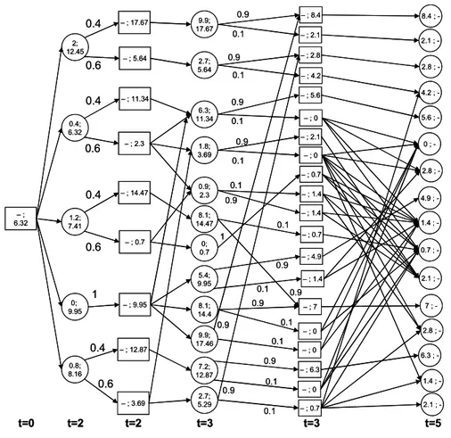
Secondly, we determine an optimal policy through a Markov Decision Process. In Figure 2.2 are reported, for each stage, the associated chance and decision states
d ,2 b ,2 1 ,2 0 ,0 a ,2 1 ,7 a,2 1 ,3 d ,2 1 ,6 b ,2 1 ,2 0 .4 0 .6 0 .4 0 .6 0.4 0 .6 1 t= 0 t= 2 t= 2 t= 3 1 ,7 a ,3 1 ,3 1 ,5 2 ,3 3 ,3 0 ,3 0 ,2 0 ,2 0 .4 0.6 b ,3 d ,3 c ,3 t= 3 2 ,1 4 1 ,7 2 ,6 a,3 2 ,1 0 1 ,3 2 ,5 d,3 2 ,3 b,3 1 ,5 2 ,1 2 3 ,3 c ,3 0,3 0 .9 0 .9 0.9 0 .9 0 .9 0 .9 1 0 .9 0 .9 0.9 0 .1 0 .1 0 .1 0.1 0 .1 0 .1 0.1 0 .1 0 .1 2 ,1 4 t= 5 1 ,7 2 ,6 a ,5 2 ,1 0 3 ,5 c ,5 1 ,5 2 ,5 b,5 d ,5 2 ,1 2 0 ,5 t= 5 0 .7 0 .3 0 .7 0 .3 0 .7 0 .3 0 .7 0 .3 0 .7 0 .3 1 0 .7 0 .3 0 .7 0 .3 0 .7 0 .3 0 .7 0 .3 0 .7 0 .3 0 .7 0 .3 0 .3 0 .7 1 ,4 1 ,4 2 ,1 1 1 ,4 0 .9 0.1 2 ,4 2 ,1 1 0 .7 0 .3 e ,3 2 ,9 e,3 0 .9 0 .1 2 ,9 e ,5 0 .7 0 .3 0 .3 0 .7 3 ,1 7 2 ,1 4 3 ,8 1 ,7 3 ,9 2 ,6 3 ,1 1 a ,5 3 ,1 3 2 ,1 0 3 ,5 e ,5 3 ,1 2 2 ,9 3 ,7 0,5 d ,5 2 ,1 1 3 ,1 4 b ,5 2 ,1 2 3 ,1 5 2 ,5 1 ,5 3 ,6 c ,5 d ,2 b ,2 1 ,2 0 ,0 a ,2 1 ,7 a,2 1 ,3 d ,2 1 ,6 b ,2 1 ,2 0 .4 0 .6 0 .4 0 .6 0.4 0 .6 1 t= 0 t= 2 t= 2 t= 3 1 ,7 a ,3 1 ,3 1 ,5 2 ,3 3 ,3 0 ,3 0 ,2 0 ,2 0 .4 0.6 b ,3 d ,3 c ,3 t= 3 2 ,1 4 1 ,7 2 ,6 a,3 2 ,1 0 1 ,3 2 ,5 d,3 2 ,3 b,3 1 ,5 2 ,1 2 3 ,3 c ,3 0,3 0 .9 0 .9 0.9 0 .9 0 .9 0 .9 1 0 .9 0 .9 0.9 0 .1 0 .1 0 .1 0.1 0 .1 0 .1 0.1 0 .1 0 .1 2 ,1 4 t= 5 1 ,7 2 ,6 a ,5 2 ,1 0 3 ,5 c ,5 1 ,5 2 ,5 b,5 d ,5 2 ,1 2 0 ,5 t= 5 0 .7 0 .3 0 .7 0 .3 0 .7 0 .3 0 .7 0 .3 0 .7 0 .3 1 0 .7 0 .3 0 .7 0 .3 0 .7 0 .3 0 .7 0 .3 0 .7 0 .3 0 .7 0 .3 0 .3 0 .7 1 ,4 1 ,4 2 ,1 1 1 ,4 0 .9 0.1 2 ,4 2 ,1 1 0 .7 0 .3 e ,3 2 ,9 e,3 0 .9 0 .1 2 ,9 e ,5 0 .7 0 .3 0 .3 0 .7 3 ,1 7 2 ,1 4 3 ,8 1 ,7 3 ,9 2 ,6 3 ,1 1 a ,5 3 ,1 3 2 ,1 0 3 ,5 e ,5 3 ,1 2 2 ,9 3 ,7 0,5 d ,5 2 ,1 1 3 ,1 4 b ,5 2 ,1 2 3 ,1 5 2 ,5 1 ,5 3 ,6 c ,5
Figure 2.2. State space of the sample problem.
(represented by circles and squares, respectively). Labels zs and Zs are shown in
0.4; 6.32 1.2; 7.41 0; 9.95 – ; 6.32 2; 12.45 – ; 17.67 – ; 5.64 – ; 11.34 – ; 2.3 – ; 14.47 – ; 0.7 – ; 9.95 0.4 0.6 0.4 0.6 0.4 0.6 1 t=0 t=2 t=2 t=3 9.9; 17.67 2.7; 5.64 6.3; 11.34 8.1; 14.47 0; 0.7 8.1; 14.4 2.7; 5.29 0.8; 8.16 – ; 3.69 0.4 0.6 0.9; 2.3 1.8; 3.69 9.9; 17.46 t=3 – ; 8.4 – ; 2.1 – ; 2.8 – ; 4.2 – ; 5.6 – ; 0 – ; 2.1 – ; 0 – ; 0.7 – ; 1.4 – ; 0.7 – ; 7 – ; 0 – ; 0 – ; 0.7 0.9 0.9 0.9 0.9 0.9 0.9 1 0.9 0.9 0.9 0.1 0.1 0.1 0.1 0.1 0.1 0.1 0.1 0.1 8.4 ; -t=5 2.1 ; 2.8 ; 4.2 ; 5.6 ; 0 ; 1.4 ; 0.7 ; 2.1 ; 2.8 ; 1.4 ; 7 ; 2.1 ; -– ; 12.87 7.2; 12.87 – ; 6.3 – ; 0 0.9 0.1 – ; 1.4 6.3 ; -5.4; 9.95 – ; 4.9 – ; 1.4 0.9 0.1 4.9 ; 2.8 ; -0.4; 6.32 1.2; 7.41 0; 9.95 – ; 6.32 2; 12.45 – ; 17.67 – ; 5.64 – ; 11.34 – ; 2.3 – ; 14.47 – ; 0.7 – ; 9.95 0.4 0.6 0.4 0.6 0.4 0.6 1 t=0 t=2 t=2 t=3 9.9; 17.67 2.7; 5.64 6.3; 11.34 8.1; 14.47 0; 0.7 8.1; 14.4 2.7; 5.29 0.8; 8.16 – ; 3.69 0.4 0.6 0.9; 2.3 1.8; 3.69 9.9; 17.46 t=3 – ; 8.4 – ; 2.1 – ; 2.8 – ; 4.2 – ; 5.6 – ; 0 – ; 2.1 – ; 0 – ; 0.7 – ; 1.4 – ; 0.7 – ; 7 – ; 0 – ; 0 – ; 0.7 0.9 0.9 0.9 0.9 0.9 0.9 1 0.9 0.9 0.9 0.1 0.1 0.1 0.1 0.1 0.1 0.1 0.1 0.1 8.4 ; -t=5 2.1 ; 2.8 ; 4.2 ; 5.6 ; 0 ; 1.4 ; 0.7 ; 2.1 ; 2.8 ; 1.4 ; 7 ; 2.1 ; -– ; 12.87 7.2; 12.87 – ; 6.3 – ; 0 0.9 0.1 – ; 1.4 6.3 ; -5.4; 9.95 – ; 4.9 – ; 1.4 0.9 0.1 4.9 ; 2.8 ;
-Figure 2.3. Expected penalties in the sample problem.
d,2 0,0 1,3 d,2 0.4 0.6 1,3 b,3 2,10 1,3 b,3 0.9 0.9 0.1 0.1 2,10 3,5 c,5 0.7 0.3 1 0.7 0.3 2,4 3,13 2,10 3,5 3,7 c,5 t=0 t=2 t=2 t=3 t=3 t=5 t=5 d,2 0,0 1,3 d,2 0.4 0.6 1,3 b,3 2,10 1,3 b,3 0.9 0.9 0.1 0.1 2,10 3,5 c,5 0.7 0.3 1 0.7 0.3 2,4 3,13 2,10 3,5 3,7 c,5 t=0 t=2 t=2 t=3 t=3 t=5 t=5
equal to Z(T0,i0,T0) = 6.32. Figure 2.4 illustrates the optimal policy which can be described as follows.
At time 0, go empty to vertex d. Wait until 2. if customer 1 requires service then
go to customer 1 (which is then serviced at time 3); no spare time is left; if customer 2 requires service then
go to customer 2 (which is then serviced at time 10); no spare time is left; if customer 3 requires service then
go to customer 3 (which is then serviced at time 13); else
end of service end
else
reposition the vehicle to vertex 2 (which it arrives at time 5); if customer 3 requires service then
service this customer (at time 5); else
end of service; end
end else
reposition the vehicle to vertex d (where it arrives at time 3); if customer 2 requires service then
go to customer 2 (which is then serviced at time 4);
reposition the vehicle in vertex c (where it arrives at time 5); if customer 3 requires service then
go to customer 3 (which is then serviced at time 7); else
end of service end
else
reposition the vehicle to vertex c (where it arrives at time 5); if customer 3 requires service then
service this customer (at time 7); else end of service; end end end
Figures 2.5 and 2.6 depict the Wait-First and Drive-First policies which yield a total expected penalty equal to 9.23 and 9.95, respectively.
2.6
Computational Results
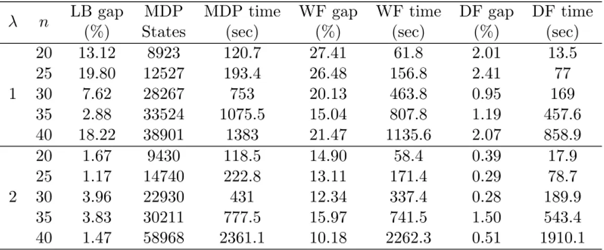
In addition, we have solved a number of randomly generated instances on a PC with a Pentium IV processor clocked at 2.8 GHz. Two sets of 50 instances were generated as follows. First, a graph G(V,A) was generated by randomly choosing points in a 100 × 100 square. Then n(⊆ |V |) customers were chosen at random and an order of visit was determined in a random fashion. In our experiments, we choose |V | = 50 and n = 20,25,30,35,40. Hence, request occurrence times were chosen as realizations of a Poisson process with λ = 1 in the first set and λ = 2 in the second set. Request probabilities were chosen as uniform random numbers in [0,1]. Computational results reported in Table 2.1 indicate that the average lower bound gap is 12.33% for λ = 1 and 2.42% for λ = 2. The Markov Decision Process was able to determine the optimal policy always within 1500 seconds for the first set and within 3000 seconds for the second set, while the number of states was always less than 40000 and 60000 for λ = 1 and λ = 2, respectively.
The average performance ratio (solution value divided by optimal policy) of the WF heuristic was 1.22 for λ = 1 and 1.13 for λ = 2. Similarly, the average performance ratio of the DF heuristic was 1.02 for λ = 1 and 1.01 for λ = 2.
Results reported in Table 2.1 show that the instances with λ = 1 were more difficult to solve, resulting in larger gaps for both the lower and upper bounding techniques and in larger computing times. This can be explained by the fact that larger arrival rates give rise to a busier vehicle. For every test set, the DF policy outperformed the WF policy both in terms of solution quality and computing time.
1,2 0,0 t=0 t=2 t=2 t=3 t=3 t=5 t=5 1,2 e,3 e,3 2,9 2,9 c,5 1 0.9 0.1 0.7 0.7 0.3 0.3 3,12 2,9 3,7 c,5 1,2 0,0 t=0 t=2 t=2 t=3 t=3 t=5 t=5 1,2 e,3 e,3 2,9 2,9 c,5 1 0.9 0.1 0.7 0.7 0.3 0.3 3,12 2,9 3,7 c,5
Figure 2.5. Drive-First policy for the sample problem.
t=0 t=2 t=2 t=3 t=3 t=5 t=5 0,2 0,0 1,4 1,4 1,4 2,11 2,11 1,5 0.4 0.9 0.1 0.7 0.7 0.3 0.3 0,2 0,3 0,3 2,6 2,6 0,5 0.7 0.7 0.3 0.3 0.6 0.9 0.1 3,14 2,11 3,6 1,5 3,9 2,6 3,8 0,5 t=0 t=2 t=2 t=3 t=3 t=5 t=5 0,2 0,0 1,4 1,4 1,4 2,11 2,11 1,5 0.4 0.9 0.1 0.7 0.7 0.3 0.3 0,2 0,3 0,3 2,6 2,6 0,5 0.7 0.7 0.3 0.3 0.6 0.9 0.1 3,14 2,11 3,6 1,5 3,9 2,6 3,8 0,5
Figure 2.6. Wait-First policy for the sample problem.
2.7
Conclusions
In this chapter we have examined exact and heuristic waiting policies for the Dy-namic and Stochastic Traveling Salesman Problem under the hypothesis that a prob-abilistic characterization of the customer requests is available. We have developed a Markov Decision Process as well as a lower bound based on the availability of perfect information. We have assessed the value of two waiting strategies against this lower bound. Our results are based on a number of assumptions that should gradually be removed: a) the hypothesis that request occurrence times T1 ≤ T2 ≤ . . . ≤ Tn
Table 2.1. Computational results
λ n LB gap MDP MDP time WF gap WF time DF gap DF time
(%) States (sec) (%) (sec) (%) (sec)
1 20 13.12 8923 120.7 27.41 61.8 2.01 13.5 25 19.80 12527 193.4 26.48 156.8 2.41 77 30 7.62 28267 753 20.13 463.8 0.95 169 35 2.88 33524 1075.5 15.04 807.8 1.19 457.6 40 18.22 38901 1383 21.47 1135.6 2.07 858.9 2 20 1.67 9430 118.5 14.90 58.4 0.39 17.9 25 1.17 14740 222.8 13.11 171.4 0.29 78.7 30 3.96 22930 431 12.34 337.4 0.28 189.9 35 3.83 30211 777.5 15.97 741.5 1.50 543.4 40 1.47 58968 2361.1 10.18 2262.3 0.51 1910.1
are sorted in non-increasing order; b) the assumption that the order of service is given; c) the hypothesis that a customer request may arise at a single time instant. These extensions are left as a future research. In addition, when removing the over mentioned hypothesis, the MDP will not be handle to handle instances with many customers. Thus, a heuristic will be needed to account for this aspect.
Chapter 3
A Priori Routes for the Dynamic
Traveling Salesman Problem
3.1
Introduction
Advances in information technology and telecommunications, together with contin-ually growing amount of data, offer opportunities for transportation companies to improve both their service offerings and the quality of the service that they provide their customers. One of the most important tools available to companies is the abil-ity to equip drivers with modern tools such as GPS devices, eventually embedded into palmtop computers, in order to exactly know where they are and also to provide them real-time directions. Another key is the ability to communicate in real-time, particularly the ability to communicate new customer requests as they happen. In addition, using the vast of amounts of data that they have stored, transportation companies have detailed statistics about their customers, including their locations and probability distributions on the time of the day that they request service.
Perhaps benefitting most from these advances in technology are delivery com-panies who emphasize same-day pick-up service. Such comcom-panies are often utilized by customers who request service with little or no notice, almost eliminating or, at least, reducing the possibility to construct the entire route in advance. To most efficiently serve these late-requesting customers, delivery companies must develop strategies which account for the late-requesting customers.
consider a single, uncapacitated vehicle serving a set of known customers locations. The choice to use an uncapacitated vehicle reflects the situation in the courier and package-express industries, where the size of parcels is small enough so that vehicle capacity is not a crucial aspect of the problem. The vehicle begins its route from a known starting point and must complete its journey at a given goal or end node (not necessarily the starting point) by a known time horizon. At the beginning of the time horizon, the driver of the vehicle is aware of a set of customers, called advance-request customers, who have already requested service. These customers may represent packages which are on the vehicle for delivery by the end of the day. In addition to the advance-request customers, there is another subset of customers, called late-request customers, such that, at the beginning of the service horizon, it is unknown whether or not they will require service.
We assume the sets of both advance- and late-request customers as well as their locations are known in advance. We also assume that we know a probability dis-tribution on the likelihood that late-request customers will request service. Our objective is to maximize the expected number of late-request customers who are served. This objective can be seen as equivalent to maximizing customers’ Quality of Service (QoS). The impact of customers’ QoS on companies is quite important, as low QoS can result in customer reimbursement or lost sales.
In trying to achieve a high-quality QoS, delivery companies face a trade-off. With any realistically-sized number of customers, exact solutions to the problem are impossible. The obvious alternative is to treat the problem entirely dynamically and to, at each decision point, decide which customer to visit next from the pool of advance-request and newly requesting late-request customers. However, this entirely dynamic approach has managerial implications in that it increases the overhead required in driver management as well as affects customer relationships associated with a driver visiting a customer at relatively the same time everyday (Campbell and Thomas, 2007 forthcoming). The alternative is to give drivers an a priori tour of advance-request customers and to insert late-request customers into this a priori tour as they request service. In this chapter, we explore the performance of various a priori routing schemes for use in the dynamic environment previously described. In the remainder of the chapter, we first describe a formal dynamic programming formulation and present the preliminary results. Then, we discuss strategies for implementing a priori routes within this dynamic routing problem as
well as our strategies for handling dynamic aspects of the problem. We next outline the experimental design and discuss the results of the computational experiments. Finally, we conclude the chapter and discuss areas for future work.
3.2
Model Formulation
In this section, we present a formal dynamic programming formulation for the described dynamic routing problem. The model mirrors the model presented in Thomas (2007), but is repeated here for completeness.
Let G = (N,E) represent the underlying network where N is the set of customers and E = N × N is the set of arcs connecting customers. For every n,n0 ∈ N, we
assume that there exists an arc (n,n0) ∈ E, including the arc (n,n). That is, the
network G is complete. Further, let tij be the amount of time required to traverse arc
(i,j) ∈ E. We can think of the time tij as deterministic or as the mean travel time
on arc (i,j). We assume 1 time unit is required to traverse a self arc. Let NJ ⊆ N
be the set of advance-request customers, customers for whom, at the beginning of the time horizon, it is known that service is required. Let NI ⊆ N be the set of
late-request customers, customers such that, at the beginning of the time horizon, it is not known whether or not n ∈ NI will require service. We assume that NI∪NJ = N
and NI∩ NJ = ∅. The vehicle begins its route at node s ∈ NJ, the start node, and
must complete its journey at a node γ ∈ NJ, the goal or end node. We note that
s 6= γ necessarily.
A decision epoch occurs when the vehicle arrives at a node. Let tk be a positive
integer representing the time of the kth decision epoch, and let n
k ∈ N be the
position of the vehicle at time tk. Let U = {0,1, . . . ,T } be the set of possible times
when decisions are made, where T is the time after which no more decisions can be made. We can think of T as the time at which the vehicle must have returned to the depot γ. Let the random variable K represent the total number of decisions and be such that, for a possible realization K of K, tK < T . Our assumptions imply that
t0 = 0,n0 = s, and K ≤ T for every possible realization of K of K.