Università degli Studi Roma Tre
Facoltà di Economia “Federico Caffè”
Scuola Dottorale Economia e Metodi Quantitativi
Dottorato in Economia Politica – XX ciclo
Essays on Dynamic Stochastic
General Equilibrium Models
Candidato: William Addessi
Supervisore: Prof. Giorgio Rodano
La stesura di questa tesi non avrebbe potuto avere luogo senza l’energia e l’intelligenza di Francesco Busato, che mi ha costantemente seguito e incoraggiato lungo tutto il lavoro di ricerca. Oltre all’aiuto tecnico volto al miglioramento del mio lavoro, la collaborazione con Francesco ha anche portato ad una bella amicizia che mi auguro continui nei prossimi anni.
Alla …ne di un percorso così importante non posso che ringraziare Giorgio Rodano, il professore che, oltre ad avermi insegnato splendidamente economia …n dal percorso di laurea, mi ha comunicato la passione per la ricerca e mi ha sempre spinto ad una comprensione critica dei fenomeni economici (e non solo di questi).
Un ringraziamento a Federico Sallusti che, oltre ad essere un grande amico, rappresenta per me l’esempio di come la passione sincera per la ricerca non debba temere di confrontarsi nè con gli schemi mentali consolidati, tanto di¤usi ed a volte tanto comodi, nè con i propri apparenti limiti.
Voglio ringraziare la mia famiglia ed i miei amici Marco, Guido e Leonardo, che mi sono stati vicini incoraggiandomi per tutti gli anni del Dottorato, senza farmi mai mancare il loro supporto ed il loro a¤etto. Inoltre ringrazio Mario Tirelli per i preziosi suggerimenti relativi al primo e terzo contributo della tesi.
In…ne, un grazie profondo va a Valeria Di Cosmo che mi è stata costantemente vic-ina, ricordandomi l’importanza dello studio dell’economia intesa come "scienza sociale" ovvero non limitata alla mera descrizione dei ‡ussi di denaro, ma come descrizione ed interpretazione dei fenomeni sociali, le cui protagoniste ultime sono le condizioni di vita dell’uomo.
Acknowledgements 1
Introduction 4
References 9
Chapter 1. Relative Preferences Shifts and Intersectoral Comovements 10
Abstract 10
1.1. Introduction 11
1.2. A Two-Sector Model with Relative-Preference Shifts 14
1.3. Numerical simulations 18
1.4. Economic Results 23
1.5. Conclusions and economic intuition 34
References 36 Appendix 38 A. Steady State 38 B. Calibration of B 39 C. Log-Linearization 39 D. Proof I 40 E. Proof II 41
Chapter 2. Bargaining Power, Labor Relations and Asset Returns 42
Abstract 42
2.1. Introduction 43
2.2. Related literature 46
2.3. Theoretical Background 47
2.4. The Economy 50
2.5. Quantitative analysis 57
2.6. Conclusions 65
References 67
Appendix 69
A. Volatility of Firm Revenue 69
B. Equilibrium Equations 70
C. Calibration 70
D. Steady State 71
E. Dynamic Equations 71
Chapter 3. Fair wages, labor relations and asset returns 72
Abstract 72
3.1. Introduction 73
3.2. Related literature 74
3.3. The Economy 80
3.4. Calibration and quantitative analysis 86
3.5. Conclusions 92
References 94
Appendix 97
A. Concavity of Labour Union’s Objective Function 97
B. Equilibrium Equations 97
C. Steady State 98
D. Calibration 98
This research theoretically analyzes some stylized facts that characterize postwar U.S. business cycles, and in particular: i) the explanation of the positive comovement of em-ployment (and other variables) across sectors; ii) the source of the di¤erence between the average real return rate on the stock market and the average riskless real interest rate (i.e. the equity premium).
Relating to the …rst theme, Christiano-Fitzgerald (1998) and Hu¤man-Wynne (1999) among others, estimate the correlation between sectoral output and employment. Their works show that output and employment across a broad range of sectors move together. With respect to the second topic, a large literature estimates that the equity market has granted, on average, substantially higher returns than Treasury bills. For example, Campbell (2002) analyzes U.S. data over the period 1947.2 to 1998.4 and asserts that the average real return has been 8.1% at annual rate, and that the average real return on 3-month Treasury bills has been 0.9% per year.
Both subjects have been largely studied in economic literature, but although the un-derstanding of these arguments has increased, some issues still deserve to be clari…ed, justifying further research on these topics.
Then the purpose of this work is to suggest a new explanation of both these themes following the dynamic stochastic general equilibrium (from now on DSGE) approach. DSGE models rely on the hypothesis that important features of the aggregate economy can be analyzed by the formalization of the behavior of representative agents (as …rms and households) that act rationally. These models generally assume the presence of exogenous shocks that generate ‡uctuations of the economic variables (such as output, employment, consumption and investment) around the long run equilibrium.
Due to the high ‡exibility of the DSGE approach, we choose to use this modelling scheme to perform our analysis for both topics of interest. Indeed, DSGE permits the formalization of a large range of hypotheses and the introduction of many elements.
Moreover, with thanks to the progress of the last decades, it allows to run numerical experiments. In this way, it is possible to calibrate the model economy so that it mimics the real economy along a carefully speci…ed set of dimensions. Then, it provides a means of studying the quantitative e¤ects of selected events.1
Thesis Overview
The …rst chapter of this work analyzes the sources of sectoral comovement. The literature that studies this topic has failed to highlight the role of consumer’s tastes as a source of positive correlation between employment in di¤erent sectors.
Indeed, this literature has mainly invoked aggregate shocks that directly a¤ect the whole economy (i.e. productivity or monetary shocks) or has highlighted the role of interlinkage in production process by conveying sectoral ‡uctuations in the entire economy. We discuss sectoral comovement by developing a two-sector model. We show that a shift in relative preferences between consumption goods is su¢ cient to explain positive comovement of output, consumption, investment and employment across sectors.
This result contrasts with the argument that in a standard business cycle model a relative preference shift between goods is followed by a negative comovement between sectoral employment.2
In order to justify how a change in the consumer’s preferences determines a shift in aggregate variables, we assume that the consumers can change their tastes with respect to their consumption goods. Then, the consumer’s satisfaction related to the entire con-sumption basket changes as well, determining a "perception e¤ect" that, under speci…c conditions, can o¤set the "substitution e¤ect" induced by the preference shift.
To explain how the mechanism works, it can be useful to consider the structure of the representative household’s preferences. The household’s utility is increasing in leisure and
1See Kydland-Prescott(1996).
consumption of two goods (denoted with c1 and c2). So the household optimally chooses both how to allocate its time between leisure and working hours in each sector and how to spend its income between the two goods.
Now suppose that the relative preferences move towards a type of consumption good that represents a small share in the consumption basket (suppose c1), then the household associates to the actual standard of consumption a lower level of satisfaction. In order to return to the optimal resource allocation, the household is willing to modify the allocation of time and income to compensate for the decrease in consumption satisfaction. Then the household proceeds as follows. It allocates time and income within the sector that produces the type of good whose relative preference has increased (i.e. c1). But, if the rise of c1is not enough to compensate the loss of satisfaction related to c2 (because now c2 has lost "appealing") then the allocation of time and income within the sector producing c2 also increases. On the contrary, if the taste change is related to some goods that are largely available to the consumer, his satisfaction from consumption increases and the dynamics are reversed. The role of the composition of the consumption basket on the household’s choice is what we identify as perception e¤ect.
Technically speaking, a preference shift directly a¤ects the marginal rate of substitution between consumption goods (in the standard way), whereas it a¤ects the marginal rate of substitution between consumption goods and leisure according to the direction of the perception e¤ect.
We show that if the shift is su¢ ciently persistent the described mechanism involves investment and labor supply in the same way, explaining a dynamic characterized by positive sectoral comovement of consumption, investment, output and employment.
It is noteworthy that the model proposed in Chapter 1 is formalized to clearly elicit the role of preference shifts. In fact, it does not consider aggregate shock, productivity shock and input-output interlinks.
The other two contributions presented in the second and the third chapters of this work develop a theoretical framework that investigates the sources of equity premium.
Most of the literature has modi…ed the preference structure of the representative agent in order to reconcile the principle of consumption smoothing with high asset returns and low, risk free rates.3
These attempts have been quite successful in replicating selected elements of …nancial variables, but they have showed some di¢ culties in explaining the behavior of wages and employment along the business cycle. In fact (as we extensively explain in Chapter 2), the standard modelling of labor supply needs highly volatile and pro-cyclical real wages in order to generate consistent equity premium. Such implication, however, is strongly rejected by empirical evidence.4
Maintaining a Consumption Capital Asset Pricing framework, we follow Danthine-Donaldson (2002) and locate the core of the explanation of the equity premium in labor relations. Although our analysis is established within this work, we propose a di¤erent institutional setting, as we investigate the interaction between labor union and …rm instead of the relation between worker and employer. Particularly, the introduction of labor unions allows disentangling labor supply from consumption path, and this hinders labor supply decisions from acting as an insurance device against ‡uctuations in consumption.
Moreover, from a theoretical point of view, the framework presented in our study allows us to incorporate insights of …nancial literature within DSGE macroeconomics models which include labor unions. 5
Detailed in Chapter 2, it is assumed that the relative bargaining power of the labor union is an increasing function of the aggregate employment rate. Under this assumption the equilibrium wage depends positively on the aggregate employment rate and on …rm’s dividend (or liquidity). We show that these two elements move in the opposite directions
3See Campbell-Cochrane (1999) for a detailed review.
4For data analysis see Christiano-Eichenbaum (1992) among others. Recently, to overcome this problem
Uhlig (2007) proposes exogenous habit formation in both leisure and consumption, and some unmodelled friction that prevents all labor supply from reaching the market.
5See Ma¤ezzoli (2001) and Chiarini-Piselli (2005) regarding the study of the role of labor union in a DSGE
model, and see Ramìrez (2006) with regard to the study the presence of labor union on …nancial market performance.
along the business cycle, and this generates a-cyclical wages. The linkage between invest-ment, dividend and wage induces high volatility on the asset returns, explaining the source of the equity premium.
Otherwise, in Chapter 3 we investigate another hypothesis concerning labor relations. We suppose that in each …rm there is a standard monopoly union, but we assume that its preferences are characterized by a concern for …rm’s performance. In particular, the union’s relative preference for wage, with respect to employment, are formalized as an increasing function of both …rm’s pro…ts and dividends. Under this assumption, the dy-namics following a productivity shock strongly depend on the chosen indicator of …rm performance.
The model is capable of explaining equity premium only when the labor union links relative preferences for wage to distributed dividends of shareholders. In fact, similar to the model proposed in the previous chapter, a relationship between investment, dividend and wage emerges, generating high volatility of asset returns and explaining the equity premium.
[1] Bencivenga, V. (1992): “An Econometric Study of Hours and Output Variation with Preference Shocks”, International Economic Review, 33 (2), 449-71.
[2] Campbell J. Y. (2002): “Consumption-Based Asset Pricing”, Harvard Institute of Economic Research, Discussion Paper Number 1974.
[3] Campbell, J. Y. and J. H. Cochrane (1999): “By Force of Habit: a Consumption-Based Explanation of Aggregate Stock Market Behavior”, Journal of Political Econ-omy, 107, 205-251.
[4] Chiarini B., and P. Piselli (2005): “Business cycle, unemployment bene…ts and pro-ductivity shocks”, Journal of Macroeconomics, 27, 670-690.
[5] Christiano L. J., and M. Eichenbaum (1992): “Current Real-Business-Cycle Theories and Aggregate Labor-Market Fluctuations”, The American Economic Review, 82(3), 430-450.
[6] Christiano, L. and T. Fitzgerald (1998): “The business cycle: It’s still a puzzle”, Economic Perspectives, Federal Reserve Bank of Chicago, issue Q IV, pages 56-83. [7] Danthine J.P., and J.B. Donaldson (2002): “Labor Relations and Asset Returns”,
Review of Economic Studies, 69, 41-64.
[8] Kydland, F. E. and E. C. Prescott: “The Computational Experiment: An Economet-ric Tool”, Journal of Economic Perspectives, 10, 1, 69-85.
[9] Hu¤man, G.W. and M. Wynne (1999): “The Role of Intratemporal Adjustment Costs in a Multisector Economy”, Journal of Monetary Economics, 43, 2, 317-50.
[10] Ma¤ezzoli M. (2001): “Non-Walrasian labor market and real business cycles”, Review of Economic Dynamics, 4, 860-892.
[11] Phelan C., and A. Trejos (2000): “The aggregate e¤ects of sectoral reallocations”, Journal of Monetary Economics, 5 (0), 7-29.
[12] Ramìrez Verdugo A. (2004), “Dividend Signaling and Unions”, Munich Personal RePEc Archive Paper n. 2273.
[13] Uhlig H. (2007): “Explaining Asset Prices with External Habits and Wage Rigidities in a DSGE Model”, American Economic Review, 97(2), 239-243
.
Relative Preferences Shifts and Intersectoral Comovements
Abstract
This paper develops a two-sector general equilibrium model in which aggregate ‡uc-tuations are driven by shocks to relative preferences between consumption goods. These shocks can be represented as possible consequences of taste changes. When such a shift in preferences occurs the consumers associate di¤erent levels of satisfaction to the same basket of consumption depending on the state of preferences. We show that, under speci…c conditions concerning the initial composition of the consumption basket, a shift in relative preferences produces a "perception e¤ect" that induces positive inter and intra sectoral comovements of selected macroeconomic variables (i.e. output, consumption, investment and employment). It is remarkable that the results are reached without introducing tech-nology shocks, input-output linkages or direct changes in relative preferences between aggregate consumption and leisure.
Journal of Economic Literature Classi…cation Numbers: F11, E320
Keywords: Demand Shocks, Two-sector Dynamic General Equilibrium Models
The positive comovement of economic activity across di¤erent sectors is one of the most important regularities of all business cycles.1 Burns-Mitchell (1946) included intersectoral comovement in the de…nition of business cycles, and many empirical studies prove pro-cyclical behavior of cross-sector measures of employment, output and investment.2 A …rst way to explain comovements along business cycles is to consider shocks that a¤ect all the economy. Proceeding in this direction it is possible to explain two important stylized facts of business cycles: persistence of deviations and positive comovements between sectors. In fact, it is generally assumed that exogenous stochastic variables follow an autoregressive process (persistence), and these shocks concern the aggregate supply or demand side of the economy (positive comovement).
This approach is not fully satisfying because it is di¢ cult to identify reasonable ag-gregate disturbances capable of explaining historical business cycles. So a vast literature emphasizes the transmission mechanisms from sectoral shocks to aggregate ‡uctuations. We follow this research …eld and propose a preference-based mechanism to explain sectoral linkages.
Most of the multi-sectoral literature considers the input-output structure of the eco-nomic system the most important transmission channel of sector-speci…c shocks. A seminal paper of Long-Plosser (1983) details a model in which the output of each sector can be used in the production process of all the other sectors, and consequently, an idiosyncratic technology shock modi…es the possibilities of the production process in each sector. How-ever, as emphasized by Murphy et al. (1989), Long-Plosser’s model explains comovements only of output and not of employment. Afterwards, many contributions have tried to explain why employment should increase in sectors that experience a reduction in relative productivity. Hornstein-Praschnik (1997) distinguish between the production of durable goods and the production of nondurable goods and highlight the great use of the latter
1Lucas (1977).
as intermediate goods in the production of the former.3 By this way, a sector-speci…c shock in either sector a¤ects the accumulation of capital (durable goods) and, therefore, the demand of intermediate goods (nondurable goods). Hu¤man-Wynne (1999) develop a two-sector model with only one sector producing capital goods to be employed in both sectors (the other type of capital goods is sector speci…c). They introduce intratemporal adjustment costs for switching production between the two types of capital. Consequently, it becomes costly to modify the composition of capital goods, and thus investment goods will be positively correlated. Horvath (1998, 2000) displays that in presence of a particular kind of not full input-use matrix, the law of large numbers does not work and then aggre-gate volatility could be induced by sector-speci…c disturbances.4 Horvath’s analysis reveals that aggregate volatility can be generated by sectoral volatility when the input-use matrix is characterized by a few full rows and many sparse columns. Thus, two requirements are needed. First, the economy has to be characterized by the presence of sectors that produce intermediate inputs for “all” the sectors of the economy. Second, only a few rows have to be full and subsequently only a few sectors have to play the role of input-supplying sectors for most of economic system.
All quoted contributions rely on both productivity shocks and technological linkages between sectors. In fact, the input-output structure grants that after an idiosyncratic productivity shock ‡uctuations in each sector have the same direction. On the contrary, Cooper-Haltiwanger (1990) suggest that the normality of demands for consumption is the channel through which sectoral shocks spread over the economy; meanwhile, the pres-ence of only a few sectors that hold inventories is the main intertemporal mechanism of transmission. For example, an increase in inventories immediately reduces the production in sectors holding inventories and then the income of workers employed in those sectors.
3The Authors support the signi…cance of their classi…cation of sectors noting that from U.S. input-output
tables it emerges that nondurable goods are 26% of total payments to inputs of the durable goods producing sector, while durable goods reach only 4% of total payments to inputs of the nondurable goods producing sector.
4The Author points out that the traditional argument against multi-sectoral models is that whether
sector-speci…c shocks are i.i.d. variables, then the law of large numbers implies that positive and negative shocks o¤set one another.
Therefore, these workers reduce the demand of the goods produced in the other sectors, thus emerging positive comovements of employment and output.
Unlike the quoted works, we develop a framework without changes to productivity. Fluctuations are induced by shocks to the structure of preferences; in particular, shocks concern consumers’ relative preference between two consumption goods. We show that such kind of preference shock is able to explain both the persistence of ‡uctuations and the positive comovements of output, consumption, investment and employment between sectors. We remark that this kind of shock a¤ects only the relative preference for di¤erent goods and does not directly modify the preference structure between the composite con-sumption good and leisure. That di¤ers from Bencivenga (1992) and Wen (2005, 2006) who assume that shocks directly a¤ect the marginal rate of substitution between consumption and leisure.
The stylized economy is characterized in the following way. Within each sector, a dis-tinct output is produced using employment and sector-speci…c capital; this sector-speci…c output yields one type of consumption good and the investment good used to accumu-late capital for the sector. This unusual assumption excludes that sectoral comovement is induced by complementarity in the production process. Utility is de…ned over leisure and over a consumption basket composed of the consumption goods from both sectors. In order to not consider a shock to the relative preference between total consumption and free time, we assume the Cobb-Douglas (homogeneous of degree 1) preferences between consumer goods. There are no other types of shocks, therefore inter and intra sectoral comovements of employment, consumption, output and investment are totally explained by shifts in relative preferences.
We interpret the dynamics focusing on di¤erent ways of perceiving the same consump-tion basket, depending on relative preferences. The paper is organized as follows. Secconsump-tion 1.2 details the benchmark economy. Section 1.3 presents the theoretical mechanism, Sec-tion 1.4 presents the selected numerical results and SecSec-tion 1.5 concludes. Finally, the Appendix includes all proofs and derivations.
1.2. A Two-Sector Model with Relative-Preference Shifts
This section presents the baseline dynamic equilibrium model with relative-preference shocks. Since there are no restrictions to trade, we solve the dynamic planning problem of a benevolent planner.
The benchmark model is structured as a two-sector, two-good economy, with endoge-nous labor supply choice. There exists a continuum of identical households of total measure one. The relative demand for goods are driven by autonomous changes in preferences of the representative household. Aggregate uncertainty originates from the demand side, and it is modelled using a state dependent utility function. Consumption and capital goods are sector speci…c, while labor services can be reallocated across sectors, without bearing any adjustment cost.
1.2.1. Preferences
De…ne a Cobb-Douglas aggregate consumption index in the following way:
Ct= c s1;t 1;t c
s2;t
2;t (1.1)
where c1;tand c2;t, respectively denote the consumption of good 1 and good 2 at time t; s1;t and s2;t denote the preference weights, following stochastic processes (de…ned below).5 In this framework, a positive shock to s1;t (i.e. an increase in s1;t) changes the instantaneous structure of preferences in favor of c1. In other words, such a shock would make the consumer perceive the commodity 1 as relatively more important with respect to the other good. The economic interpretation of this kind of shock is immediate. A preference shift is like a change in tastes. If we interpret c1 as a speci…c kind of good, for example clothes, cars or food, and c2 as the remaining goods composing the consumption basket, a positive shock to s1 implies that the relative preference for clothes (or cars or food) increases with respect to the relative preference for the other goods. In the following section, it will be analyzed how the relative weight of c1 in the consumption basket,
5Also Stockman-Tesar (1995) use the Cobb-Douglas aggregator for tradable consumption goods in a two
a¤ects the way the consumer "feels" immediately after the shock. This feeling represents the key element to explain positive comovement in our framework. In order to highlights the aggregate e¤ects of only relative shocks, we preserve the homotheticity of degree 1 of preferences and assume that s1;t+ s2;t = 1, 8 all t = 1; 2; :::.
Preferences over aggregate consumption index Ct and leisure `t are described by a state dependent felicity function u(C (ct) ; `t; st) : R2+ S2 [0; 1]
2 ! R:
u(ct; `t; st) =
(Ct)1 1
1 + B`t; (1.2)
where is a parameter that measures the degree of risk aversion and is inversely propor-tional to the elasticity of intertemporal substitution; `tdenotes leisure hours. In order to better understand the behavior of demands for consumption goods, we assume that the marginal utility of leisure is constant and equal to B.6 Leisure hours are de…ned as:
`t= 1 n1;t n2;t (1.3)
where n1;t and n2;t denote working hours in sector 1 and 2. It implies that available hours are normalized to 1 and labor services shift across sectors without adjustment costs.
1.2.2. Production Technologies
Each good is produced with physical capital and labor, using a sector-speci…c Cobb-Douglas technology: y1;t = 1k1;t1n 1 1 1;t and y2;t = 2k2;t2n 1 2 2;t ; (1.4)
where kj;t and j denote, respectively, capital stock and technology level in sector j, for j = 1; 2. There is no exogenous technology process ( i.e. j parameters are constant over time) so the production is not subject to exogenous technology shocks. As remarked in the introduction, this strongly di¤erentiates our model from the traditional approach that focuses on the e¤ects of idiosyncratic productivity shocks.
6In a following section we show that linearity in leisure is not a necessary condition. Such assumption
In each sector, capital accumulation follows the standard formulation
k1;t+1= (1 1)k1;t+ i1;t and k2;t+1= (1 2)k2;t+ i2;t; (1.5)
where the jdenotes depreciation rates of capital stocks and ij;tdenotes investment ‡ows at time t, for j = 1; 2. Eq.(1.4) and eq.(1.5) dictate that the investment good for the capital stock used in sector j is produced entirely in sector j. This hypothesis makes capital goods …xed across sectors and then rules out input-output transmission mechanisms. In this way, it is possible to isolate the way preferences drive intersectoral comovements with no in‡uences from production processes. If we assume that the output of a sector can be used in the production of the other sector, we could observe a positive comovement with no clear understanding of the role of preferences.
The allocation constraint is speci…c for each sector and is given by
c1;t+ i1;t = y1;t and c2;t+ i2;t = y2;t; (1.6)
1.2.3. Preference Shocks
As just explained, we preserve the homotheticity of degree 1 of preferences and assume that s1;t+ s2;t = 1. Then, it is su¢ cient to specify the characteristics of s1. It follows an autoregressive process, s1;t+1= s1;t+ (1 ) s1+ "t, where 0 1 and s1 is the steady state value. "t is a random variable characterized by the following degenerated distribu-tion "t+h= 100s1 for h = 0, "t+h= 0 8 h > 0 . Consequently the relative-preference shock f"1;tg1t=1 is transitory, but because of the preference structure, it has persistent e¤ects. Roughly speaking, we are analyzing the e¤ects of a one-shot shock to relative preferences on the stylized economy.
1.2.4. Model’s Solution and Equilibrium Characterization
Planner maximizes the expected present discounted value of the return function V0 = E0P1t=0 tu(ct; `t; st), where (0 < < 1) is a subjective discount factor, subject to the allocation constraints (eq.(1.6)), the capital accumulation constraints (eq.(1.5)), and
the total-hour constraint (eq.(1.3)). The state of the economy at time t is represented by a vector t = hk1;t; k2;t; s1;t; s2;ti. Controls for the problem are consumption ‡ows c, investment ‡ows i, and the labor services n. Introducing dynamic multipliers 1;t and
2;t, forming the Hamiltonian H yields:
max fcj;t;nj;t;kj;t+1g2j=1;nt H = E0 1 X t=0 t 8 > < > : cs1;t1;t cs2;t2;t 1 1 1 + B (1 n1;t+ n2;t) + + 1;th 1k1;t1n 1 1 1;t c1;t+ (1 1) k1;t k1;t+1 i + + 2;th 2k2;t2n 1 2 2;t c2;t+ (1 2) k2;t k2;t+1 io ; (1.7)
where E0 is the conditional expectation operator on time 0 information. First order conditions with respect to j-th consumption ‡ow and working hours (FOC(cj;t), FOC(nj;t) for j = 1; 2 hereafter) read:
c1;t : s1;tc s1;t 1 1;t c s2;t 2;t c s1;t 1;t c s2;t 2;t = 1;t c2;t : s2;tcs1;t1;t c2;ts2;t 1 cs1;t1;t cs2;t2;t = 2;t (1.8) n1;t : B = 1;t(1 1) 1k1;t1n1;t1 n2;t : B = 2;t(1 2) 2k2;t2n2;t2 (1.9)
where (1 j) jkj;tjnj;t j = wj;t is the marginal productivity of labor in sector j. Combining the previous equations, the FOCs for both consumption goods can be rewritten as: s1;t Ct1 c1;t w1;t = B s2;t Ct1 c2;t w2;t = B (1.10)
Optimality conditions (eq.(1.10)) indicate the standard equality between the weighted marginal utility of consumption (sj;tC
1 t
c1;t ) and the weighted marginal utility of leisure (wj;tB ). Notice that if > 1, the sectoral consumption is negatively related to the aggregate consumption index.
After little simple algebra, investment dynamics are determined by the following two Euler Equations: Et s1;t+1 Ct+11 c1;t+1w1;t+1 s1;t Ct1 c1;t w1;t 1 1k1;t+11 1n 1 1 1;t+1+ (1 1) = 1 Et s2;t+1 Ct+11 c2;t+1w2;t+1 s2;tC 1 t c2;t w2;t 2 2k2;t+12 1n 1 2 2;t+1+ (1 2) = 1 (1.11)
where Et denotes the expectations operator, conditional on information available at time t. Notice that the pricing kernel j;t =
Ct+11 Ct1
sj;t+1cj;t
sj;tcj;t+1 is a¤ected by the relative-preference
parameters and it depends on both the level of consumption of the speci…c kind of good and the level of consumption index.
Combining optimal conditions and resource constraints we determine the deterministic steady state.7 Then we proceed to log-linearize the model around the steady state to study the dynamics.8 In the next section we illustrate the parameterization of the model and then we show the results.
1.3. Numerical simulations 1.3.1. Parameterization
The system of equations we use to compute the dynamic equilibrium of the model depends on a set of twelve parameters. Six pertain to technology (the capital share in both sectors j, the capital stock quarterly depreciation rate j, the equilibrium value of technology j), while the other six pertain to consumer’s preferences (the subjective discount factor , the relative risk aversion coe¢ cient , the marginal utility of leisure B, the relative
7See the Appendix.
preference for good 1, s1, and for good 2, s2, and the autoregressive coe¢ cient of the relative preference process ).9
The two sectors are characterized by the same production process, so the eventual di¤erences between equilibrium values derive from consumers’ preferences. So sectoral technology parameters are set perfectly equal in both sectors. This assumption makes it easy to associate the parameterization of the relative preferences to the composition of the consumption index. In fact, under the symmetric hypothesis concerning the supply side, it emerges that c1 R c2 , s1 R s2. Assuming di¤erences in the supply side, it would complicate the exposition of the mechanisms with no signi…cant added value in the understanding of the role of preferences. The model is parameterized for the U.S. economy based on the post-war period, apart of relative preference parameters that are set to develop the theoretic investigation. The parameterization reads:
Technology parameters ( j; j; j) are set to commonly used values in RBC lit-erature. We consider a symmetric economy by the supply side so, 1 = 2 = 0:025,
1 = 2= 0:36 and 1= 2 = 1.
Consumer’s preference ( ; ; B; sj; ) : the quarterly subjective discount factor is set to correspond to an annual real interest rate of 4%; it yields = 0:99. The relative risk aversion is equal to 5. The relative preference for good 1, s1, varies in the range 0 < s1 < 1 but in the baseline version is set equal to 0:1. The autoregressive coe¢ cient of the preference process is 0:99. The marginal utility of leisure, B is endogenously calibrated to generate n1+ n2 = 0:3.10
1.3.2. Structure of the simulation exercises
In this section we investigate how the stylized economy responses to an increase in the relative preference for good 1. We assume a temporary 1% positive deviation of s1 from the steady state value. Here we anticipate that, in our framework, the key element that determines the rise of comovement, is the ratios1s2. Then, the …rst set of simulations reports impulse responses for di¤erent values of s1s2. Precisely, the di¤erent values of this ratio are:
9Recall that the preference parameter for good 2, s2, is set equal to 1 s1.
s1 s2 = 1 (s1 = 0:5 and s2 = 0:5), s1 s2 < 1 (s1 = 0:1 and s2 = 0:9) and s1 s2 > 1 (s1 = 0:9 and s2 = 0:1). These simulations help to show how the e¤ects of a preference shock change according to the initial structure of preferences. To explain the emerging results, we need to introduce what we call "perception e¤ ect " that we consider the main element inducing positive inter-sectoral comovement after a preference shock. As we will explain later in the paper, the perception e¤ect is related to the di¤erent levels of satisfaction that the representative household can attribute to the same consumption basket according to the state of preferences. Then we conduce sensitivity analysis to study the role of the parameters that characterize the dynamics of the model. From the sensitivity analysis the following results will emerge. Firstly, the autoregressive coe¢ cient of the preference shock principally a¤ects the responses of investments, because it determines how long the immediate impact on consumptions extends to the future. Secondly, the coe¢ cient of intertemporal substitution 1, together with the ratio s1s2, determines if the perception e¤ect is su¢ ciently high to outrun the substitution e¤ect following a preference shock (i.e. we will show that the value of is very important to make emerge positive inter-sectoral comovement). Finally we will remove the linearity assumption concerning the preferences for leisure. As well, we will show that such assumption is not necessary and that the characterization of preferences for leisure contributes to strengthening or weakening inter-sectoral comovements without signi…cantly modifying economic mechanisms.
1.3.3. Baseline simulations
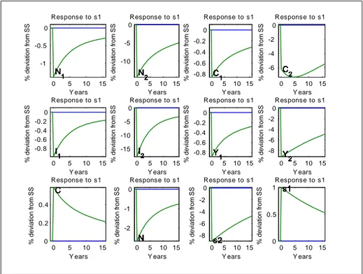
Initially, we run the model three times maintaining the baseline calibration with the ex-ception of the steady state value of s1.11 We set s1 equal to 0:5, to 0:1 (the benchmark value) and to 0:9 and report results respectively in Figure 1.1, Figure 1.2 and Figure 1.3.
0 5 10 15 0 0.5 1 Response to s1 Y ears % dev iat ion from SS NNNNNNNNNNNN111111111111 0 5 10 15 -1 -0.5 0 Response to s1 Y ears % dev iat ion from SS N2 N2 N2 N2 N2 N2 N2 N2 N2 N2 N2 N2 0 5 10 15 0 0.2 0.4 0.6 Response to s1 Y ears % dev iat ion from SS C 1 C 1 C 1 C 1 C 1 C 1 C 1 C 1 C 1 C 1 C 1 C 1 0 5 10 15 -0.6 -0.4 -0.2 0 Response to s1 Y ears % dev iat ion from SS C 2 C 2 C 2 C 2 C 2 C 2 C 2 C 2 C 2 C 2 C 2 C 2 0 5 10 15 0 0.5 1 1.5 Response to s1 Y ears % dev iat ion from SS IIIIIIIIIIII111111111111 0 5 10 15 -1.5 -1 -0.5 0 Response to s1 Y ears % dev iat ion from SS I 2 I 2 I 2 I 2 I 2 I 2 I 2 I 2 I 2 I 2 I 2 I 2 0 5 10 15 0 0.2 0.4 0.6 0.8 Response to s1 Y ears % dev iat ion from SS YYYYYYYYYYYY111111111111 0 5 10 15 -0.8 -0.6 -0.4 -0.2 0 Response to s1 Y ears % dev iat ion from SS Y 2 Y 2 Y 2 Y 2 Y 2 Y 2 Y 2 Y 2 Y 2 Y 2 Y 2 Y 2 0 5 10 15 0 0.05 0.1 Response to s1 Y ears % dev iat ion from SS C C C C C C C C C C C C 0 5 10 15 0 0.05 0.1 Response to s1 Y ears % dev iat ion from SS N N N N N N N N N N N N 0 5 10 15 -1 -0.5 0 Response to s1 Y ears % dev iat ion from SS s2 s2 s2 s2 s2 s2 s2 s2 s2 s2 s2 s2 0 5 10 15 0 0.5 1 Response to s1 Y ears % dev iat ion from SS s1s1s1s1s1s1s1s1s1s1s1s1
Figure 1.1. s1 = 0:5 (Perfectly symmetric model)
0 5 10 15 0 0.5 1 1.5 Response to s1 Y ears % dev iat ion from SS NNNNNNNNNNNN111111111111 0 5 10 15 0 0.05 0.1 0.15 Response to s1 Y ears % dev iat ion from SS NNNNNNNNNNNN222222222222 0 5 10 15 0 0.2 0.4 0.6 0.8 Response to s1 Y ears % dev iat ion from SS CCCCCCCCCCCC111111111111 0 5 10 15 0 0.05 0.1 Response to s1 Y ears % dev iat ion from SS CCCCCCCCCCCC222222222222 0 5 10 15 0 0.5 1 1.5 Response to s1 Y ears % dev iat ion from SS IIIIIIIIIIII111111111111 0 5 10 15 0 0.05 0.1 Response to s1 Y ears % dev iat ion from SS IIIIIIIIIIII222222222222 0 5 10 15 0 0.5 1 Response to s1 Y ears % dev iat ion from SS YYYYYYYYYYYY111111111111 0 5 10 15 0 0.05 0.1 Response to s1 Y ears % dev iat ion from SS YYYYYYYYYYYY222222222222 0 5 10 15 -0.05 0 0.05 0.1 Response to s1 Y ears % dev iat ion from SS C C C C C C C C C C C C 0 5 10 15 0 0.1 0.2 Response to s1 Y ears % dev iat ion from SS NNNNNNNNNNNN 0 5 10 15 -0.1 0 0.1 Response to s1 Y ears % dev iat ion from SS s2 s2 s2 s2 s2 s2 s2 s2 s2 s2 s2 s2 0 5 10 15 0 0.5 1 Response to s1 Y ears % dev iat ion from SS s1s1s1s1s1s1s1s1s1s1s1s1 Figure 1.2. s1 = 0:1
0 5 10 15 -1 -0.5 0 Response to s1 Y ears % dev iat ion from SS N 1 N 1 N 1 N 1 N 1 N 1 N 1 N 1 N 1 N 1 N 1 N 1 0 5 10 15 -10 -5 0 Response to s1 Y ears % dev iat ion from SS N 2 N 2 N 2 N 2 N 2 N 2 N 2 N 2 N 2 N 2 N 2 N 2 0 5 10 15 -0.8 -0.6 -0.4 -0.2 0 Response to s1 Y ears % dev iat ion from SS C 1 C 1 C 1 C 1 C 1 C 1 C 1 C 1 C 1 C 1 C 1 C 1 0 5 10 15 -6 -4 -2 0 Response to s1 Y ears % dev iat ion from SS C2 C2 C2 C2 C2 C2 C2 C2 C2 C2 C2 C2 0 5 10 15 -0.8 -0.6 -0.4 -0.2 0 Response to s1 Y ears % dev iat ion from SS I 1 I 1 I 1 I 1 I 1 I 1 I 1 I 1 I 1 I 1 I 1 I 1 0 5 10 15 -15 -10 -5 0 Response to s1 Y ears % dev iat ion from SS I2 I2 I2 I2 I2 I2 I2 I2 I2 I2 I2 I2 0 5 10 15 -0.8 -0.6 -0.4 -0.2 0 Response to s1 Y ears % dev iat ion from SS Y1 Y1 Y1 Y1 Y1 Y1 Y1 Y1 Y1 Y1 Y1 Y1 0 5 10 15 -8 -6 -4 -2 0 Response to s1 Y ears % dev iat ion from SS Y 2 Y 2 Y 2 Y 2 Y 2 Y 2 Y 2 Y 2 Y 2 Y 2 Y 2 Y 2 0 5 10 15 0 0.2 0.4 Response to s1 Y ears % dev iat ion from SS CCCCCCCCCCCC 0 5 10 15 -2 -1 0 Response to s1 Y ears % dev iat ion from SS N N N N N N N N N N N N 0 5 10 15 -8 -6 -4 -2 0 Response to s1 Y ears % dev iat ion from SS s2 s2 s2 s2 s2 s2 s2 s2 s2 s2 s2 s2 0 5 10 15 0 0.5 1 Response to s1 Y ears % dev iat ion from SS s1s1s1s1s1s1s1s1s1s1s1s1 Figure 1.3. s1 = 0:9
Detailed, within the …gures are reported the impulse response functions of employment (N1, N2), consumption (C1, C2), investment (I1, I2) and output (Y1, Y2) of both sectors; C is the aggregate consumption index as de…ned in eq.(1.1), N is the total employment and the last two boxes refer to the preference weights for consumption goods12.
Figure 1.1 (with s1 = s2 = 0:5) shows an economy where input factors (N2 and I2) are withdrawn from the production of good 2 (Y2 and C2 decrease) and are allocated to sector 1. Intra sectoral comovements between consumption, investment, employment and output are positive in both sectors, but inter-sectoral comovements are negative. In fact, the sector characterized by an increase in preference (sector 1) goes through an expansive phase while the other sector goes through a recessive phase.
Figure 1.2 (with s1 = 0:1, s2= 0:9) shows an economy with both sectors in expansion. Both inter-sectoral and intra sectoral comovements are positive.
Figure 1.3 (with s1 = 0:9, s2 = 0:1), similar to Figure 1.2, shows an economy char-acterized by both positive inter-sectoral and positive intra-sectoral comovements, but the dynamics are completely reversed. The stylized economy experiences a recession in both
sectors and in all variables (consumption, investment, employment and output). Reported …gures raise some questions that need an explanation.
1.4. Economic Results
1.4.1. In which cases do preference shifts generate positive inter and intra sectoral comovement of consumption and employment?
The key element to understand the di¤erent dynamics reported above is the impulse response function of the aggregate consumption index C. It represents a …rst measure of the representative household’s felicity. In fact, assuming a standard utility function (i.e. increasing and concave in consumption), the behavior of C a¤ects both the level of satisfaction and the marginal utility associated with the consumption of each good.13 To better understand the role of the aggregate index, assume that a shock to preferences occurs and that c1 and c2 are …xed. Notwithstanding, the value of the consumption index changes because of preference parameters. Therefore, the total and marginal utilities related to each good and to the aggregate index also change. In this scenario, we will show that the marginal utility of C is the key element that could induce positive inter-sectoral comovements and aggregate ‡uctuations. First, let’s try to make clear the economic intuition and then describe the mechanism more analytically.
Roughly speaking, we can argue that the in‡uence of cj on consumer’s utility (i.e. the marginal utility of cj) is given by the e¤ect of cj on C and the e¤ect of C on the utility. If preferences shift, both of the e¤ects vary but only the latter can induce positive inter-sectoral comovement. In fact, in the previous three examples (reported in Figures 1.1-1.3), after the positive shock to s1 the ceteris paribus e¤ect of c1 on C increases while the e¤ect of c2 on C decreases.14 This is a sort of "substitution e¤ ect " that acts in the standard direction: after a positive shock to s1 the representative consumer desires to substitute good 2 for good 1. On the contrary, it is not unique the way the in‡uence of
13In our model C does not a¤ect marginal utility of leisure because we assume that the utility function is
separable in consumption and leisure.
14In the Appendix we prove that Cc
1s1 > 0 and that Cc2s1 < 0to show that only the direct e¤ect of
the shock on C can explain positive inter-sectoral comovements. This is con…rmed also by the impulse
C on the utility changes, because it depends on the way C changes after the shock. If C decreases (increases) then the marginal impact of C on utility increases (decreases). We call this change "perception e¤ ect " that a¤ects the marginal rate of substitution between consumption (consumption index and single good consumption) and any other argument of the utility function, as leisure in this case. In other words, C does not in‡uence the marginal rate of substitution between c1 and c2, but in‡uences the marginal rate of sub-stitution between ci and leisure (1 n1 n2).15
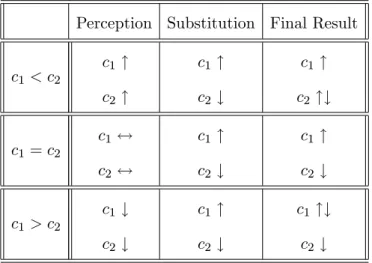
So, when C falls because of the preference shift (independently on what happens to c1 and c2), the marginal utility of consumption index increases and this positively in‡uences the marginal utility of both consumption goods. This scenario is in accordance to Figure 1.2. The reverse occurs in Figure 1.3: the marginal utility of consumption index has reduced so highly that also sector 1 experiences a negative phase. In both cases positive sectoral comovements emerge driven by sectoral (and not aggregate) preference shock. The following table resumes possible scenarios after a positive shock to s1.
Table 1.1 Possible dynamics of consumption after a positive shock to s1
Perception Substitution Final Result
c1 < c2 c1 " c2 " c1 " c2 # c1 " c2 "# c1 = c2 c1 $ c2 $ c1 " c2 # c1 " c2 # c1 > c2 c1 # c2 # c1 " c2 # c1 "# c2 #
15The preference shock generates a sort of "real wealth e¤ ect ", if it is assumed that real wealth can be
measured by the level of utility that consumer can reach. In fact, after the shock the level of satisfaction has changed because the consumer associates di¤erent satisfaction to the same goods. So, the level of satisfaction changes even if the consumption choices are unchanged. But it is necessary to note that even if we adopt the previous de…nition, the mechanism proposed in this paper is quite di¤erent from that emerging in standard microeconomic problems. This is because the …rst element to change is not the budget constraint but the indi¤erence curve.
Now, let’s try to develop more analytically the argument. Consider the optimal con-dition ruling the choice between consumption and leisure in each sector (with j = 1; 2),
Ucjwj = UCCcjwj = B (1.12)
Equation (1.12) imposes that in equilibrium the marginal utility of consumption of good j, Ucj, weighted with the marginal productivity of labor in sector j, wj, has to be equal to the marginal utility of leisure, B.16 The marginal utility of cj can be decomposed in the product between the …rst derivative of the utility function with respect to the aggregate consumption index, UC (i.e. the marginal utility of C), and the …rst derivative of such index with respect to the single consumption good, Ccj. The key question concerns what happens to UC after an increase in s1 (as in our simulations). To answer, it is necessary to focus on the signs of two derivatives. The …rst is the sign of the …rst derivative of the marginal utility UCwith respect to the consumption index (i.e. the second derivative of the utility function with respect to the consumption index). This sign is univocal negative (in fact, UCC = C 1 < 0).
The second sign concerns the derivative of the consumption index with respect to the exogenous shock, Cs1.17 The sign of this derivative depends on the ratio between the consumption goods composing the consumption index, in fact Cs1 = cs11 c
1 s1
2 ln(c1c2). Recall that in our model the supply sides of the sectors are perfectly symmetric; it follows that the relative dimension of steady state values of sectoral variables depends only on consumer’s preferences. Then c1 R c2 i¤ s1 R s2. In the benchmark version (reported in Figure 1.2) s1 = 0:1 so c1c2 < 1, and then Cs1 < 0. If C # then UC ". In this case, the direct e¤ect of a positive shock to s1 reduces C and then increases UC. So, according to the optimal conditions (eq.(1.12)) the product between Ccjwj has to fall in both sectors, given the marginal utility of leisure, B. This can occur by an increase in cj (the derivative
16Assuming B constant, the dynamic equation of eq.(1.12) can be expressed in the following way: ~sj;t
ecj;t+ (1 ) eCt+ jekj;t jenj;t= 0. This equation is very helpful to follow the mechanism described in the present section.
17We are interested in the direct e¤ect of s1 on C taking the rest as given. So we are not considering the
of Ccj with respect to cj is negative, in fact Cc1c1 = s1(s1 1) cs11 2c 1 s1
2 < 0, Cc2c2 = s1(1 s1) cs11 c
s1 1
2 < 0) and also by an increase in employment nj (to reduce wj).18 This mechanism contributes in explaining the positive inter-sectoral comovements re-ported in Figure 1.2 and in Figure 1.3 and why the economic booms (dooms) occur after a preference shock when s1 is set low (high).
Finally, Figure 1.1 represents the case of a perfectly symmetric economy: s1 = 0:5, c1
c2 = 1, Cs1 = 0. The direct e¤ect of preferences on UC is null; so the dynamics of the economy is simply driven by substitution e¤ects between sectoral goods. In this case the marginal rate of substitution between leisure and consumption index does not change and neither the aggregate employment does.
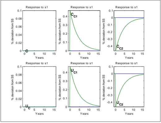
As con…rmation, consider these other …gures that report the impulse responses of other variables (with the exception of the consumption index, C).19 "Cc1" and "Cc2" are the …rst derivative of C with respect to c1 and c2.20 "UC" is the …rst derivative of the utility function with respect to the consumption index, and its dynamics describe the behavior of perception e¤ect.21 Finally, "Uc1" and "Uc2" are the marginal utilities with respect to c1 and c2.22
Figure 1.4 con…rms that in the symmetric case with no perception e¤ect the marginal utility of each good depends only on the way the good a¤ects the consumption index.2 3
18It is noteworthy that it is also relevant the way C varies because of sectoral speci…c consumption changes
(Ccj). So Cs1 does not explain the entire variation of UC.
19These tables are indicated as "bis" because they replicate the corresponding previous exercises.
20Cc 1 = s1c s1 1 1 c 1 s1 2 and Cc2= (1 s1) c s1 1 c s1
2 and the dynamic equations are respectively 0 = Cce1+
[1 + s1ln(c1 c2)]es1+ (s1 1)ec1+ (1 s1)ec2 and 0 = Cce2+ [ s1 1 s1+ s1ln( c1 c2)]es1+ s1ec1 s1ec2 where the
tilde indicates the variation rate of the variable. To simplify we have substituited s2 = 1 s1.
21UC= C and the dynamic equation is 0 = UCe C;e
22Uc
1 = UCCc1 and Uc2 = UCCc2 and the dynamic equations are 0 = Uce1 + eUC + eCc1 and 0 =
e
Uc2+ eUC+ eCc2.
2 3Re¤ering to note (18), notice that in this case C does not varies because Cs
1 = 0 but also because
Figure 1.5 and Figure 1.6 show two cases in which the perception e¤ect is so high that it o¤sets the substitution e¤ect. In the case with s1 = 0:1 (Figure 1.5) the perception e¤ect works in the same direction of the substitution e¤ect for good 1 but in the opposite direction for good 2. Consequently, the response of "Uc1" is stronger than the response of "Cc1", while the response of "Uc2" is reversed with respect to the response of "Cc2" (because the perception e¤ect predominates). In the case with s1= 0:9 the reverse occurs; in fact, despite the increase in the relative preference for good 1, the marginal utility of c1 decreases while the marginal utility of c2 strongly falls.24
0 5 10 15 0 0.02 0.04 0.06 0.08 0.1 Response to s1 Y ears % dev iat ion from SS C C C C C C 0 5 10 15 0 0.1 0.2 0.3 0.4 Response to s1 Y ears % dev iat ion from SS CC1 CC1 CC1 CC1 CC1 CC1 0 5 10 15 -0.4 -0.3 -0.2 -0.1 0 0.1 Response to s1 Y ears % dev iat ion from SS CC2 CC2 CC2 CC2 CC2 CC2 0 5 10 15 0 0.02 0.04 0.06 0.08 0.1 Response to s1 Y ears % dev iat ion from SS U C U C U C U C U C U C 0 0 5 10 15 0.1 0.2 0.3 0.4 Response to s1 Y ears % dev iat ion from SS UC1 UC1 UC1 UC1 UC1 UC1 0 5 10 15 -0.4 -0.3 -0.2 -0.1 0 0.1 Response to s1 Y ears % dev iat ion from SS U C2 U C2 U C2 U C2 U C2 U C2
Figure 1.4. s1 = 0:5 (Perfectly symmetric model)
24Notice that Figure 1.5 and Figure 1.6 are not perfectly symmetric because the entity of the shock is
di¤erent. Respectively 1% of 0:1 and 1% of 0:9. Notwithstanding, the comparison of the relative responses are very similar.
0 5 10 15 -0.05 0 0.05 0.1 Response to s1 Y ears % dev iat ion from SS C C C C C C 0 5 10 15 -0.1 -0.05 0 0.05 0.1 0.15 0.2 Response to s1 Y ears % dev iat ion from SS C C1 C C1 C C1 C C1 C C1 C C1 0 5 10 15 -0.25 -0.2 -0.15 -0.1 -0.05 0 0.05 Response to s1 Y ears % dev iat ion from SS C C2 C C2 C C2 C C2 C C2 C C2 0 5 10 15 0 0.05 0.1 0.15 0.2 0.25 0.3 Response to s1 Y ears % dev iat ion from SS U C U C U C U C U C U C 0 5 10 15 0 0.1 0.2 0.3 0.4 0.5 Response to s1 Y ears % dev iat ion from SS U C1 U C1 U C1 U C1 U C1 U C1 0 5 10 15 0 0.02 0.04 0.06 0.08 0.1 Response to s1 Y ears % dev iat ion from SS U C2 U C2 U C2 U C2 U C2 U C2 Figure 1.5. s1 = 0:1 0 5 10 15 0 0.1 0.2 0.3 0.4 0.5 Response to s1 Y ears % dev iat ion from SS C C C C C C 0 5 10 15 0 0.5 1 1.5 2 Response to s1 Y ears % dev iat ion from SS C C1 C C1 C C1 C C1 C C1 C C1 0 5 10 15 -2 -1.5 -1 -0.5 0 0.5 Response to s1 Y ears % dev iat ion from SS C C2 C C2 C C2 C C2 C C2 C C2 0 5 10 15 -2.5 -2 -1.5 -1 -0.5 0 Response to s1 Y ears % dev iat ion from SS UC UC UC UC UC UC 0 5 10 15 -0.5 -0.4 -0.3 -0.2 -0.1 0 0.1 Response to s1 Y ears % dev iat ion from SS U C1 U C1 U C1 U C1 U C1 U C1 0 5 10 15 -5 -4 -3 -2 -1 0 Response to s1 Y ears % dev iat ion from SS U C2 U C2 U C2 U C2 U C2 U C2 Figure 1.6. s1 = 0:9
In this section we have not described all the forces determining the dynamics of this stylized economy, because we are principally interested in the mechanisms that induce pos-itive inter-sectoral comovements. So, as evidenced in Table 1.1 (by the use of arrows), the ratio between preference parameters (or consumption goods) represents a sort of necessary, but not su¢ cient, condition to observe positive inter-sectoral comovements in response to relative-preference shifts.
1.4.2. And what about investment choice?
To answer we need two other sets of impulse response functions. Starting from the bench-mark calibration (with s1 = 0:1 and = 0:99, reported in Figure 1.2), reduce the au-toregressive coe¢ cient of preference process to = 0:92 and to = 0:80. Results are represented respectively in the following two …gures (Figure 1.7 and Figure 1.8).
0 5 10 15 0 0.2 0.4 0.6 0.8 Response to s1 Y ears % dev iat ion from SS NNNNNNNNNNNN111111111111 0 5 10 15 0 0.05 0.1 Response to s1 Y ears % dev iat ion from SS N 2 N 2 N 2 N 2 N 2 N 2 N 2 N 2 N 2 N 2 N 2 N 2 0 5 10 15 0 0.2 0.4 0.6 0.8 Response to s1 Y ears % dev iat ion from SS C 1 C 1 C 1 C 1 C 1 C 1 C 1 C 1 C 1 C 1 C 1 C 1 0 5 10 15 0 0.05 0.1 Response to s1 Y ears % dev iat ion from SS C2 C2 C2 C2 C2 C2 C2 C2 C2 C2 C2 C2 0 5 10 15 -0.4 -0.2 0 Response to s1 Y ears % dev iat ion from SS I1 I1 I1 I1 I1 I1 I1 I1 I1 I1 I1 I1 0 5 10 15 0 0.05 0.1 Response to s1 Y ears % dev iat ion from SS I 2 I 2 I 2 I 2 I 2 I 2 I 2 I 2 I 2 I 2 I 2 I 2 0 5 10 15 0 0.2 0.4 Response to s1 Y ears % dev iat ion from SS YYYYYYYYYYYY111111111111 0 5 10 15 0 0.05 0.1 Response to s1 Y ears % dev iat ion from SS Y2 Y2 Y2 Y2 Y2 Y2 Y2 Y2 Y2 Y2 Y2 Y2 0 5 10 15 -0.05 0 0.05 0.1 Response to s1 Y ears % dev iat ion from SS C C C C C C C C C C C C 0 5 10 15 0 0.05 0.1 0.15 Response to s1 Y ears % dev iat ion from SS NNNNNNNNNNNN 0 5 10 15 -0.1 0 0.1 Response to s1 Y ears % dev iat ion from SS s2 s2 s2 s2 s2 s2 s2 s2 s2 s2 s2 s2 0 5 10 15 0 0.5 1 Response to s1 Y ears % dev iat ion from SS s1s1s1s1s1s1s1s1s1s1s1s1 Figure 1.7. = 0:92
It is immediately noted that the impulse responses of consumptions and outputs are less persistent (it would be strange if the opposite occurred). Another evidence is that the selected changes in the value of the persistence parameter from the preference process
0 5 10 15 0 0.2 0.4 Response to s1 Y ears % dev iat ion from SS N 1 N 1 N 1 N 1 N 1 N 1 N 1 N 1 N 1 N 1 N 1 N 1 0 5 10 15 0 0.05 0.1 Response to s1 Y ears % dev iat ion from SS N 2 N 2 N 2 N 2 N 2 N 2 N 2 N 2 N 2 N 2 N 2 N 2 0 5 10 15 0 0.5 1 Response to s1 Y ears % dev iat ion from SS C1 C1 C1 C1 C1 C1 C1 C1 C1 C1 C1 C1 0 5 10 15 0 0.05 0.1 Response to s1 Y ears % dev iat ion from SS C 2 C 2 C 2 C 2 C 2 C 2 C 2 C 2 C 2 C 2 C 2 C 2 0 5 10 15 -1.5 -1 -0.5 0 Response to s1 Y ears % dev iat ion from SS I1 I1 I1 I1 I1 I1 I1 I1 I1 I1 I1 I1 0 5 10 15 -0.05 0 0.05 0.1 Response to s1 Y ears % dev iat ion from SS I2 I2 I2 I2 I2 I2 I2 I2 I2 I2 I2 I2 0 5 10 15 0 0.1 0.2 0.3 Response to s1 Y ears % dev iat ion from SS Y1 Y1 Y1 Y1 Y1 Y1 Y1 Y1 Y1 Y1 Y1 Y1 0 5 10 15 0 0.05 0.1 Response to s1 Y ears % dev iat ion from SS Y2 Y2 Y2 Y2 Y2 Y2 Y2 Y2 Y2 Y2 Y2 Y2 0 5 10 15 -0.05 0 0.05 0.1 Response to s1 Y ears % dev iat ion from SS C C C C C C C C C C C C 0 5 10 15 0 0.05 0.1 Response to s1 Y ears % dev iat ion from SS N N N N N N N N N N N N 0 5 10 15 -0.1 0 0.1 Response to s1 Y ears % dev iat ion from SS s2 s2 s2 s2 s2 s2 s2 s2 s2 s2 s2 s2 0 5 10 15 0 0.5 1 Response to s1 Y ears % dev iat ion from SS s1 s1 s1 s1 s1 s1 s1 s1 s1 s1 s1 s1 Figure 1.8. = 0:80
does not reverse the sign of inter-sectoral comovements. In fact these are still positive in both cases.
To our aim, the most important e¤ect of a reduction in concerns the change in the intra-sectoral comovements; in fact investments gradually become counter-cyclical with respect to the other variables. The negative correlation between consumption and investment is due to the quicker return to the original consumption index. In fact, after the preference shock the representative consumer "feels worse" and prefers reducing leisure to increase consumption. If the preference process is highly persistent, this feeling is long lasting and then it is optimal to plan a long lasting increase in consumption. Immediately this aim needs both higher consumption and higher investment. On the contrary, if the preference process is not highly persistent, the consumer needs to increase only actual consumption because the marginal rate of substitution between actual leisure and future consumption (to say actual investment) does not change signi…cantly. Then, with low values of , actual consumption increases in detriment to both actual leisure and future
consumption, while when = 0:99 actual and future consumption increase in detriment to actual leisure.25
Again, it is worth noticing that in this model the investment good for the capital stock used in sector j is produced entirely in sector j. This means that di¤ering from labor services, capital is not mobile across sectors. Such assumption is fundamental to eliminate every kind of input-output linkage between sectors. In this way, the emerging inter-sectoral comovements are not generated by a combination of technological and preference reasons, but they are entirely due to preference shifts. In fact, relaxing this hypothesis the transfer of capital goods would ease the explication of inter-sectoral comovements of outputs and investments.
1.4.3. The role of the intertemporal elasticity of substitution in consumption Regarding the role of , the impulse response functions continue to be a very clarifying instrument. So, we maintain the benchmark calibration and substitute = 5 with = 1:5. The dynamics after a shock to s1 are reported in Figure 1.9.
0 5 10 15 0 0.5 1 Response to s1 Y ears % dev iat ion from SS NNNNNNNNNNNN111111111111 0 5 10 15 0 0.05 0.1 Response to s1 Y ears % dev iat ion from SS N 2 N 2 N 2 N 2 N 2 N 2 N 2 N 2 N 2 N 2 N 2 N 2 0 5 10 15 0 0.2 0.4 0.6 Response to s1 Y ears % dev iat ion from SS CCCCCCCCCCCC111111111111 0 5 10 15 0 0.05 0.1 Response to s1 Y ears % dev iat ion from SS C 2 C 2 C 2 C 2 C 2 C 2 C 2 C 2 C 2 C 2 C 2 C 2 0 5 10 15 0 0.5 1 1.5 Response to s1 Y ears % dev iat ion from SS IIIIIIIIIIII111111111111 0 5 10 15 -0.05 0 0.05 0.1 Response to s1 Y ears % dev iat ion from SS I2 I2 I2 I2 I2 I2 I2 I2 I2 I2 I2 I2 0 5 10 15 0 0.2 0.4 0.6 0.8 Response to s1 Y ears % dev iat ion from SS YYYYYYYYYYYY111111111111 0 5 10 15 0 0.05 0.1 Response to s1 Y ears % dev iat ion from SS Y 2 Y 2 Y 2 Y 2 Y 2 Y 2 Y 2 Y 2 Y 2 Y 2 Y 2 Y 2 0 5 10 15 -0.1 0 0.1 Response to s1 Y ears % dev iat ion from SS C C C C C C C C C C C C 0 5 10 15 0 0.05 0.1 Response to s1 Y ears % dev iat ion from SS NNNNNNNNNNNN 0 5 10 15 -0.1 0 0.1 Response to s1 Y ears % dev iat ion from SS s2 s2 s2 s2 s2 s2 s2 s2 s2 s2 s2 s2 0 5 10 15 0 0.5 1 Response to s1 Y ears % dev iat ion from SS s1s1s1s1s1s1s1s1s1s1s1s1 Figure 1.9. = 1:5
25The impulse responses con…rm the entire argument. For example, observe that the immediate deviation
The …gure shows that with low values of the positive comovements between sectors vanish. The reason is that the importance of the perception e¤ect has decreased. Analyz-ing the dynamic equation of the …rst derivative of the utility function with respect to the consumption index ( eUC = C), or considering dynamic equation reported in note (16),e it is clear that is a scale factor of the e¤ect of C on the marginal utility of consumption. So if is low, variations in C poorly a¤ect the relative preference between consumption goods and leisure and thus inter-sectoral comovements are infrequent.
1.4.4. The role of the intertemporal elasticity of substitution in leisure
The model has been developed assuming that the marginal utility of leisure is constant. The assumption serves a speci…c purpose. It permits to isolate the substitution and perception e¤ects in consumption with no variation in marginal utility of leisure.
But this assumption is not necessary. In fact, we can solve the model assuming the following utility function: u(ct; `t; st) = (Ct)
1 1
1 +
1
vB(1 n1;t n2;t)
v, where (1 v)
controls the degree of the risk aversion and is inversely proportional to the elasticity of intertemporal substitution in leisure. Obviously, with v = 1 the model collapses in eq.(1.2). To analyze the in‡uence of v, we set v = 0:2 and then v = 1, and run the model in the usual way. Results are reported in the following …gures.
Figure 1.10 and Figure 1.11 indicate that decreasing v (to say decreasing the in-tertemporal elasticity of leisure), it becomes less frequent to observe positive inter-sectoral comovements. Clearly, this parameter does not directly modify the relative weight of perception e¤ect and substitution e¤ect. The di¤erent dynamics emerge because of the behavior of the marginal utility of leisure that, with v < 1, is positively related to la-bor supply. In fact, even if the perception e¤ect is su¢ ciently high to generate positive dynamics of the marginal utility of good 2, the positive inter-sectoral comovements are dampened by the increase in the marginal utility of leisure. As shown in the …gures, the representative household is less inclined to reduce leisure time, so the increase in time employed in sector 2 reduces and the e¤ects are particularly signi…cant for investment in this sector.
0 5 10 15 0 0.5 1 1.5 Response to s1 Y ears % dev iat ion from SS NNNNNNNNNNNN111111111111 0 5 10 15 0 0.05 0.1 Response to s1 Y ears % dev iat ion from SS NNNNNNNNNNNN222222222222 0 5 10 15 0 0.2 0.4 0.6 0.8 Response to s1 Y ears % dev iat ion from SS CCCCCCCCCCCC111111111111 0 5 10 15 0 0.05 0.1 Response to s1 Y ears % dev iat ion from SS C 2 C 2 C 2 C 2 C 2 C 2 C 2 C 2 C 2 C 2 C 2 C 2 0 5 10 15 0 0.5 1 1.5 Response to s1 Y ears % dev iat ion from SS IIIIIIIIIIII111111111111 0 5 10 15 0 0.05 0.1 Response to s1 Y ears % dev iat ion from SS I 2 I 2 I 2 I 2 I 2 I 2 I 2 I 2 I 2 I 2 I 2 I 2 0 5 10 15 0 0.2 0.4 0.6 0.8 Response to s1 Y ears % dev iat ion from SS YYYYYYYYYYYY111111111111 0 5 10 15 0 0.05 0.1 Response to s1 Y ears % dev iat ion from SS Y2 Y2 Y2 Y2 Y2 Y2 Y2 Y2 Y2 Y2 Y2 Y2 0 5 10 15 -0.05 0 0.05 0.1 Response to s1 Y ears % dev iat ion from SS C C C C C C C C C C C C 0 5 10 15 0 0.1 0.2 Response to s1 Y ears % dev iat ion from SS NNNNNNNNNNNN 0 5 10 15 -0.1 0 0.1 Response to s1 Y ears % dev iat ion from SS s2 s2 s2 s2 s2 s2 s2 s2 s2 s2 s2 s2 0 5 10 15 0 0.5 1 Response to s1 Y ears % dev iat ion from SS s1s1s1s1s1s1s1s1s1s1s1s1 Figure 1.10. v = 0:2 0 5 10 15 0 0.5 1 Response to s1 Y ears % dev iat ion from SS NNNNNNNNNNNN111111111111 0 5 10 15 0 0.05 0.1 Response to s1 Y ears % dev iat ion from SS N2 N2 N2 N2 N2 N2 N2 N2 N2 N2 N2 N2 0 5 10 15 0 0.2 0.4 0.6 Response to s1 Y ears % dev iat ion from SS CCCCCCCCCCCC111111111111 0 5 10 15 0 0.05 0.1 Response to s1 Y ears % dev iat ion from SS C 2 C 2 C 2 C 2 C 2 C 2 C 2 C 2 C 2 C 2 C 2 C 2 0 5 10 15 0 0.5 1 1.5 Response to s1 Y ears % dev iat ion from SS IIIIIIIIIIII111111111111 0 5 10 15 -0.1 0 0.1 Response to s1 Y ears % dev iat ion from SS I2 I2 I2 I2 I2 I2 I2 I2 I2 I2 I2 I2 0 5 10 15 0 0.2 0.4 0.6 0.8 Response to s1 Y ears % dev iat ion from SS YYYYYYYYYYYY111111111111 0 5 10 15 0 0.05 0.1 Response to s1 Y ears % dev iat ion from SS Y 2 Y 2 Y 2 Y 2 Y 2 Y 2 Y 2 Y 2 Y 2 Y 2 Y 2 Y 2 0 5 10 15 -0.05 0 0.05 0.1 Response to s1 Y ears % dev iat ion from SS C C C C C C C C C C C C 0 5 10 15 0 0.05 0.1 0.15 Response to s1 Y ears % dev iat ion from SS NNNNNNNNNNNN 0 5 10 15 -0.1 0 0.1 Response to s1 Y ears % dev iat ion from SS s2 s2 s2 s2 s2 s2 s2 s2 s2 s2 s2 s2 0 5 10 15 0 0.5 1 Response to s1 Y ears % dev iat ion from SS s1s1s1s1s1s1s1s1s1s1s1s1 Figure 1.11. v = 1
1.5. Conclusions and economic intuition
In this model we have studied theoretical implications of shocks to relative prefer-ences between consumption goods. We have shown that if preference structure is strongly asymmetric, positive inter and intra sectoral comovements could be generated by relative-preference shifts. Moreover, we have shown that results are consistent with respect to di¤erent kinds of sensitivity analysis. A strong implication of the model is that positive employment comovements can be explained by sectoral shocks without the introduction of input-output linkages.
The sketched mechanism is quite new in economic literature. In fact, positive co-movements of economic sectors are generally explained by either a kind of input-output structure that transmits sectoral shocks over the entire economy or a kind of aggregate shocks. In the last …eld Bencivenga (1992) and Wen (2005, 2006) can also be inserted, who consider direct variations in relative preference between consumption and leisure. In fact, in the cited works, independently of the composition of consumption basket, the relative importance of consumption with respect to leisure is subject to change. This can be due to the fact that leisure time is employed in other activities (as homework production, see Benhabib et al., 1990), or it can be induced by alternative phases of the level of "con-sumerism" (or of "the urge to consume", see Wen, 2006) that modi…es the importance of consumption. On the contrary, our model does not explicitly focus on consumerism but indicates two elements: the starting composition of consumption basket and the shifts in relative preference between consumption goods26. If preferences shift to a (kind of) good that represents a highly minor or a highly major share of the actual consumption basket, then business cycles with positive sectoral comovements could emerge27. The …rst case (minor share) can be represented in the following way. Suppose that the representative consumer increases the preference for a good that actually concerns a little share of her
26Phelan-Trejos (2000) investigate preference shifts between consumption goods, but they …nd negative
comovement in sectoral employment. It is very interesting that they observe changes in the sector not a¤ected by the preference shock (their model considers three sectors), and they guess the relevance of the complementarity of consumption goods, but they do not see that the complementarity of consumption goods can generate positive comovement of sectoral employment.
27In section(1.4.1) we have shown that aggregate booms and dooms are more frequent when the values of
consumption; she increases the demand for this good but she still gets an amount of it that is perceived as not enough to maintain the previous level of satisfaction. Consequently, to compensate such lack of satisfaction related to consumption, the consumer increases the demand for the other goods too. A particularly interesting implication of the model concerns the e¤ects of advertising. In fact, this model suggests that the attempt to capture consumers’ preferences can generate "not obvious e¤ects". For example, supposing that s1 is high (low), and interpreting positive shocks to s1 as a consequence of advertising of sector 1, the model predicts that we could observe a reduction (increase) in the demand for good 1 (good 2). This opens other research …elds that lie outside this model.