supervised machine learning
of ultracold atoms with speckle
disorder
s. pilati
1& p. pieri
1,2We analyze how accurately supervised machine learning techniques can predict the lowest energy levels of one-dimensional noninteracting ultracold atoms subject to the correlated disorder due to an optical speckle field. Deep neural networks with different numbers of hidden layers and neurons per layer are trained on large sets of instances of the speckle field, whose energy levels have been preventively determined via a high-order finite difference technique. The Fourier components of the speckle field are used as the feature vector to represent the speckle-field instances. A comprehensive analysis of the details that determine the possible success of supervised machine learning tasks, namely the depth and the width of the neural network, the size of the training set, and the magnitude of the regularization parameter, is presented. It is found that ground state energies of previously unseen instances can be predicted with an essentially negligible error given a computationally feasible number of training instances. First and second excited state energies can be predicted too, albeit with slightly lower accuracy and using more layers of hidden neurons. We also find that a three-layer neural network is remarkably resilient to Gaussian noise added to the training-set data (up to 10% noise level), suggesting that cold-atom quantum simulators could be used to train artificial neural networks.
Machine learning techniques are at the heart of various technologies used in every day life, like e-mail spam filtering, voice recognition software, and web-text analysis tools. They have already acquired relevance also in physics and chemistry research. In these fields, they have been employed for diverse tasks, including: finding energy-density functionals1–4, identifying phases and phase transitions in many-body systems5–11, predict-ing properties such as the atomization energy of molecules and crystals from large databases of known com-pounds12–14, or predicting ligand-protein poses and affinities for drug-design research15–18. Among the various machine learning methodologies, supervised machine learning has been put forward as a fast, and possibly accu-rate, technique to predict the energies of quantum systems exploiting the information contained in large datasets obtained using computationally expensive numerical tools19.
Computational physicists and chemists have already demonstrated that supervised machine learning can be used, in particular, to determine the potential energy surfaces for molecular dynamics simulations of materials, of chemical compounds, and of biological systems20–26. This allows one to avoid on-the-fly quantum mechanical electronic-structure computations, providing a dramatic speed-up that makes larger scale simulations of complex systems as, e.g., liquid and solid water, feasible27. However, it is not yet precisely known how accurately the statis-tical models commonly employed in supervised machine learning can describe quantum systems. In general, the accuracy achievable by these statistical models, chiefly artificial neural networks, depends on various important details, including the depth and the connectivity structure of the neural network, the size of the training set, and the type of regularization employed during the training process to avoid the pervasive over-fitting problem28. Also the choice of the features adopted to represent the quantum system of interest plays a crucial role; in fact, substantial research work has been devoted to the development of efficient representations (see, e.g., refs17,29,30). It is natural to expect that addressing models that describe highly tunable and easily accessible experimental setups could shed some light on this important issue.
These considerations lead us to focus on ultracold atom experiments. These systems have emerged in recent years as an ideal platform to investigate quantum many-body phenomena31,32. They allowed experimental-ists to implement archetypal Hubbard-type models of condensed matter physics33 and even the realization of
1School of Science and Technology, Physics Division, Università di Camerino, 62032, Camerino, (MC), Italy. 2infn,
Sezione di Perugia, 06123, Perugia, (PG), Italy. Correspondence and requests for materials should be addressed to S.P. (email: [email protected])
Received: 15 October 2018 Accepted: 21 March 2019 Published: xx xx xxxx
programmable simulators of quantum spin Hamiltonians34. One can envision the use of these analog quantum simulators as computational engines to create datasets to be fed to supervised machine learning methods, provid-ing data to train artificial neural networks even for models that defeat computational techniques. One example is the fermionic Hubbard model, that has been implemented in various cold-atom laboratories35–37. In fact, recent cold-atom quantum simulations of the Hubbard-model have been analyzed via machine learning techniques38.
One of the quantum phenomena that received most consideration by cold-atom researchers is the Anderson localization transition in the presence of disorder39–43. This phenomenon consists in the spatial localization of the single particle states, determining the absence of transport in macroscopic samples44. Unlike conventional con-densed matter systems, which inherently include a certain amount of impurities, in cold-atom setups disorder is introduced on purpose. The most frequently used technique consists in creating optical speckle fields by shining lasers through rough semitransparent surfaces, and then focusing them onto the atomic cloud. These speckle fields are characterized by a particular structure of the spatial autocorrelation of the local optical field inten-sities45,46. These correlations have to be accounted for in the modeling of cold-atom experiments with speckle fields47,48. Indeed, they determine the position of the mobility edge49–51, namely the energy threshold that in three dimensional systems separates the localized states from the extended ergodic states. In low dimensional configurations, any amount of disorder is sufficient to induce Anderson localization. However, the speckle-field correlations determine the transport properties and even the emergence of so-called effective mobility edge, i.e. energy thresholds where the localization length changes abruptly52–54.
In this article we perform a supervised machine learning study of the lowest three energy levels of a one-dimensional quantum particle moving in a disordered external field. This model is designed to describe an alkali atom exposed to a one-dimensional optical speckle filed, taking into account the detailed structure of the spatial correlations of the local intensities of the speckle field. This is in fact the setup implemented in the first cold-atom experiments on Anderson localization39,40. The first task we address is to determine the energy levels of a large set of speckle-field instances via a high-order finite difference formula. Next, we train a deep artificial neural network to reproduce the energy levels of this training set, and we then employ the trained neural network to predict the energy levels of previously unseen speckle-field instances.
The main goals of this study are (i) to analyze how accurately deep neural networks can predict low-lying energy levels of (previously unseen) system instances, (ii) to quantify how this accuracy depends on the depth and width of the network, (iii) to verify if and how the overfitting problem can be avoided, and how large the training set has to be to achieve this, (iii) to check if and how accurately excited state energies can be predicted, compared to ground-state energy levels. Furthermore, in view of the possible future use of cold-atom quantum simulators to provide data for supervised machine learning tasks, we analyze if and to what extent deep neural networks are resilient with respect to noise present in the training data. Such noise is indeed an unavoidable feature of any experimental outcome.
The main result we obtain is that, given a computationally affordable number of system instances for training, a neural network with three hidden layers can predict ground state energies of new system instances with a mean quadratic error well below 1% (relative to the expected variance); this error appears to systematically decrease with training-set size. Higher energy levels can be predicted too, but the accuracy of these predictions is slightly lower and requires the training of deeper neural networks. We also show that if one has only small or moderately large training sets (including order of 103 instances, as in some previous machine learning studies) the overfit-ting problem does indeed occur, and it has to be minimized via an appropriate regularization, that we quantify. Another important finding we report here is that a deep neural network (with three layers of hidden neurons) is extremely robust against noise in the training set, providing essentially unaffected predictions for previously unseen instances up to almost 10% noise level in the training data.
Model
The model we consider is defined by a Hamiltonian operator that in coordinate representation reads: = − + ˆH m x V x 2 d d ( ), (1) 2 2 2 d
where ħ is the reduced Planck’s constant and m the particle mass. Vd(x) is a disordered external field, designed to represent the potential energy of an atom subject to an optical speckle field. Experimentally, these optical fields are generated when coherent light passes through, or is reflected by, rough surfaces. In the far field regime, a spe-cific light intensity pattern develops, commonly referred to as optical speckle field. In cold-atom experiments, this optical speckle field is focused onto the atomic cloud using a converging lens.
A numerical algorithm to generate the intensity profile of a speckle field is based on the following expression55:
ξ ϕ ξ
= | − | .
V xd( ) V F W F0 1[ ( ) [ ]( )]( )x 2 (2) Here, the constant V0 corresponds to the average intensity of the speckle field, while we denote with
∫
ϕ ξ = ϕ − πξ
F[ ]( ) d ( )x x e i2 x (3)
the Fourier transform of the complex field ϕ(x), whose real and imaginary part are independent random variables sampled from a Gaussian distribution with zero mean and unit variance. F−1 indicates the inverse Fourier trans-form. The function W(ξ) is a filter defined as
ξ ξ ξ = | | ≤ | | > W w w ( ) 1 if /2 0 if /2, (4)
where w is the aperture width, which depends on the details of the optical apparatus employed to create and focus the speckle field, namely the laser wavelength, the size (illuminated area) and the focal length of the lens employed for focusing. We consider blue detuned optical fields, for which the constant V0 introduced in Eq. (2) is positive.
In the numerical implementation, the Gaussian random complex field ϕ(x) is defined on a discrete grid:
xg = gδx, where δx = L/Ng, L is the system size, and the integer g = 0, 1, …, Ng − 1. The number of grid points
Ng shall be large, as discussed below. The continuous Fourier transform is henceforth replaced by the discrete version. Periodic boundary conditions are adopted, and the definition (2) is consistent with this choice, i.e.
Vd(L) = Vd(0).
For a large enough systems size L, the optical speckle field is self-averaging, meaning that spatial averages coincide with the average of local values over many instances of the speckle field, indicated as 〈Vd(x)〉d. These instances are realized by choosing different random numbers to define the complex field ϕ(x). The probability distribution of the local speckle-field intensity Vloc = Vd(x), for any x, is P(Vloc) = exp(−Vloc/V0)/V0 for Vloc≥0,
and P(Vloc) = 0 otherwise. It follows that, for large enough L, the average speckle-field intensity 〈Vd(x)〉d = V0 is equal to the standard deviation 〈V xd( )2〉 −V =V
d 02 0. Therefore, V0 is the unique parameter that determines the amount of disorder in the system.
The local speckle-field intensities at different positions have statistical correlations, characterized by the fol-lowing spatial autocorrelation function:
π π
Γ( )x = 〈V x V xd( ) (′ d ′ + 〉x V) / 02− =1 [ sin( wx)/( wx)]2. (5) One notices that the inverse of the aperture width w determines the correlation length, i.e. the typical size of the speckle grains. We will indicate this length scale as γ = w−1, which corresponds to the first zero of the cor-relation function Γ(x). The corcor-relation length allows one to define an energy scale, dubbed corcor-relation energy, defined as Ec = ħ2/(2mγ2).
In the following we consider the system size L = 20γ, with a number of grid points Ng = 1024. Notice that with this choice one has δxγ, so that the discretization effect is irrelevant. Furthermore, the speckle-field intensity is fixed at the moderately large value V0 = 5Ec. We point out that we choose to normalize the optical speckle field so that its spatial average over the finite system size L exactly corresponds to V0, for each individual instance, thus eliminating small fluctuations due to finite size effects.
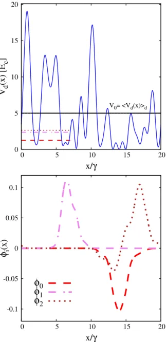
The local intensity profile of a typical instance of optical speckle field is displayed in the upper panel of Fig. 1. The continuous horizontal line indicates the average intensity V0. The lower panel displays the three eigenfunc-tions φi(x), with i = 0, 1, 2, corresponding to the lowest energy levels. They solve the Schrödinger equation
ϕ = ϕ
ˆH xi( ) ei i( )x with eigenvalues ei. These energy levels are indicated by the three horizontal segments in the upper panel of Fig. 1. The wave functions and the corresponding energy levels are computed via a finite difference approach, employing the grid points xg defined above, using a highly accurate 11-point finite difference formula. This makes the discretization error negligible. One notices that the wave functions φi(x) have non-negligible values only in a small region of space. This is consistent with the Anderson localization phenomenon, which in one-dimensional configurations is expected to occur for any amount of disorder, as predicted by the scaling the-ory of Anderson localization56. Indeed, one might also notice that the node of the wave function corresponding to the first excited state is in a region of vanishing amplitude and is therefore barely visible.
Clearly, the energy levels ei randomly fluctuate for different instances of the speckle field. Their probability dis-tribution is shown in Fig. 2, where the averages over many speckle-field instances 〈ei〉d are also indicated with ver-tical segments. One notices that the probability distribution of the ground-state energy e0 is slightly asymmetric, while the distributions of the excited energy levels e1 and e2 appear to be essentially symmetric. Other properties of quantum particles in an optical speckle field, such as the density of states, have been investigated in refs47,57.
Methods
The first step in a supervised machine learning study consists in choosing how to represent the system instances. One has to choose Nf real values that describe the system, all together constituting the so-called features vector. One natural choice would consist in choosing the speckle field values Vd(xg) on the Ng points of the spatial grid defined in Sec. 1. Indeed, if the grid is fine enough these values fully define the system Hamiltonian. However, since Ng has to be large, this choice leads to a pretty large features vector, making the training of a deep neural network with many neurons and many layers rather computational expensive. This approach was in fact adopted in a recent related article19. The problem of the large feature vector was circumvented by employing so-called convolutional neural networks. In such networks the connectivity structure is limited. This reduces the number of parameters to be optimized, making the training more computationally affordable. The connectivity structure is in fact designed so that the network can recognize the spatial structures in the feature vector, somehow auto-matically extracting the relevant details from a large feature space.
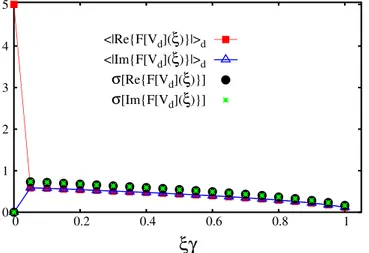
In this article we adopt a different strategy. The definition of the optical speckle field in Eq. (2) and the struc-ture of the spatial correlations described in Sec. 1 suggest that one can construct a more compact system rep-resentation by switching to the Fourier space. In fact, it is easy to show that the (discrete) Fourier transform of the speckle field F[Vd](ξ) has a finite support, limited to the interval ξ∈[−w:w]. This limits the number of nonzero Fourier components. Since the Fourier grid spacing is δξ = 1/L, one expects to have 42 nonzero (complex) Fourier components for our choice of system size L = 20γ. One should also consider that the Fourier transform of a real
signal has the symmetry F[Vd](−ξ) = F[Vd](ξ)*. This further limits the number of nonzero independent variables, leaving us with a feature vector with only Nf = 42 (real) components. In Fig. 3 we plot the average over many speckle-field instances of the absolute value of the real and imaginary parts of the Fourier components F[Vd](ξ). Only the positive semiaxis ξ ≥ 0 is considered, due to the symmetry mentioned above. It should also be pointed out that due to the choice of normalization discussed in Sec. 1, the real part of the Fourier transform at ξ = 0 is fixed at Re{F[Vd](0)} = 5Ec, for each individual speckle-field instance; also, the imaginary part is fixed at Im{F[Vd] (0)} = 0. This reduces the number of active features to 40. Still, we include all Nf = 42 components in the feature vector, in view of future studies extended to speckle fields with varying intensities. In fact, the inactive features do not play any role in the training of the neural network.
In supervised machine learning studies it is sometimes convenient to normalize the components of the feature vector so that they have the same minimum and maximum values, or the same mean and standard deviation. This improves the efficiency in those cases in which the bare (non-normalized) feature values vary over scales that dif-fer by several orders of magnitude. However, as can be evinced by the plot of their standard deviations (denoted
σ[Re{F[Vd](ξ)}] and σ[Im{F[Vd](ξ)}]) in Fig. 3, the Fourier components of the speckle field differ at most by a factor of ~4. Therefore a normalization procedure is not required here.
Figure 1. Upper panel: local intensity Vd(x) of a typical instance of optical speckle field, as a function of the spatial coordinate x/γ. The energy unit is the correlation energy Ec = ħ2/(2mγ2), defined by the spatial correlation length of the speckle field γ. The continuous horizontal (black) line indicates the average over many speckle-field instances of the optical speckle field intensity V0 = 〈Vd(x)〉d. Lower panel: profile of the three lowest-energy wave functions of the speckle field instance displayed in the upper panel. The corresponding energy levels are indicated by the three horizontal segments in the upper panel.
Our plan is to train the neural network to predict the three lowest energy levels of a quantum particle in a speckle field. We generate a large number of speckle-field instances (we indicate this number with Nt) using dif-ferent random numbers, as discussed in Sec. 1. Their energy levels are computed via the finite difference approach (see Sec. 1). The target value is either the ground-state energy, or the first excited energy level, or the second energy level. Actually, for mere convenience, we consider the shifted energy levels y = εi = ei − 〈ei〉d (with i = 0, 1, 2), so that the target values have zero mean when averaged over many speckle-field instances. Each instance is represented by the feature vector =f ( , ,f f1 2 …,fNf), namely the Nf = 42 values taken from the nonzero Fourier components described above, and the target value y (ground state, first excited state, or second excited state) to be learned.
The statistical model we consider is a feed-forward artificial neural network, as implemented in the multi-layer perceptron regressor of the python scikit-learn library58. This neural network includes various layers with a spec-ified number of neurons. The leftmost layer is the input layer. It includes Nf neurons, each representing one of the features values. Next, there is a tunable number of hidden layers; we indicate this number as Nl. This is one of the details of the statistical model that will be analyzed. The number of neurons in the hidden layers, indicated as Nn, can also be tuned. (Different hidden layers could have different numbers of neurons. However, in this article we choose to have the same number of neurons Nn in all hidden layers.) Nn is the second relevant detail of the statis-tical model to be analyzed. The input layer and the hidden layers also include a bias term. The rightmost layer is the output layer, and includes one neuron only. Each neuron h = 1, …, Nn in the hidden layer l = 1, …, Nl takes a value ahl obtained by evaluating the so-called activation function, denoted by g(⋅), on the weighted sum ∑ w a−
j h jl, jl 1
of the values of the neurons in the previous layer l − 1, adding also the bias term bhl, leading to:
=
(
∑ − +)
ahl g j h jw al, jl 1 bhl . The index j labels neurons in the previous layer, so that j = 1, …, Nf when l = 1 and 0 0.2 0.4 0.6 0.8 1 1.2 0 0.5 1 1.5 2 2.5 3 3.5 4 4.5 <e0>d <e1>d<e2>d
P(e
i)
e
i[E
c]
e
0e
1e
2Figure 2. Probability distribution P(ei) of the first three energy levels e0, e1, and e2. The vertical segments indicate the corresponding averages over many speckle-field instances 〈e0〉d, 〈e1〉d, and 〈e2〉d. The energy unit is the correlation energy Ec.
Figure 3. Average over many speckle-field instances of the absolute value of the Fourier components of
the speckle field. The (red) squares correspond to the real part. The (blue) open triangles correspond to the imaginary part. The (black) circles and the (green) stars indicate the standard deviations of the real part and of the imaginary part, respectively.
j = 1, …, Nn when l > 1. The coefficients wh jl, are the weights between layer l and layer l − 1, with l = 1, …, Nl + 1. They represent the model parameters that have to be optimized during the learning process, together with the bias terms bhl. The neuron of the output layer (corresponding to the index l = Nl + 1) also performs the weighted sum with bias, but the activation function is here just the identity function. Taking, as an illustrative example, a neural network with one hidden layer and one neuron in the hidden layer, the learning function would be
=
(
∑ +)
+F f() w g1,12 jw f1,1j j b11 b12. Different choices for the activation function g(x) of the hidden neurons are
possible, including, e.g., the identity, the hyperbolic tangent, and the rectified linear unit function, defined as
g(x) = max(0, x). In this article, we adopt the latter function. A preliminary analysis has shown that other suitable
choices perform quite poorly.
The training process consists in optimizing the model parameters wh jl, and bhl so that the function values F(ft) closely approximate the target values yt. Here, the index t = 1, …, Nt labels the instances in the training set. The optimization algorithm is designed to minimize the loss function L( )W = ∑21 t( ( )Fft −yt))2+ 12α W 22, where
the second term is the regularization and is introduced to penalize complex models with large coefficients. It is computed with the L2-norm, indicated as ⋅ 2, of the vector W, which includes all weight coefficients. The regu-larization is useful to avoid overfitting, the situation in which the target values of the training instances are accu-rately reproduced, but the neural network fails to correctly predict the target values of previously unseen instances. The magnitude of the regularization term can be tuned by varying the (positive) regularization param-eter α. Typically, large values of α are required to avoid the pervasive over-fitting problem when the training set is small (if the neural network has many layers and many hidden neurons), while small (or even vanishing) values of α can be used if the training set is sufficiently large. The role of this parameter is another important aspect that will be analyzed below.
The optimization is performed using the Adam algorithm59, an improved variant of the stochastic gradient descent method, which is readily implemented in the scikit-learn library, and proves to perform better than the other available options for our problem. The tolerance parameter in the multi-layer perceptron regressor is set to 10−10, providing a large parameter for the maximum number of iteration so that convergence is always reached. All other parameters of the multi-layer perceptron regressor are left at their default values.
Results
In the following, we evaluate the performance of the trained neural network in predicting the energy levels of a set of Np = 40000 speckle-field instances not included in the training set. As a figure of merit, we consider the coefficient of determination, typically denoted with R2, defined in the general case as:
= −∑ − ∑ − = = R F y y y f 1 ( ( ) ) ( ) , (6) p N p p p N p 2 1 2 1 2 p p
where = ∑y N1p Np=p1yp is the average of the target values in the test set, which is essentially zero here due to the use
of shifted energy levels. A perfectly accurate statistical model which exactly predicts the target values of all the instances in the test set would yield a coefficient of determination equal to R2 = 1. For example, a constant func-tion which produces (only) the correct average of the test set target values, but (clearly) completely fails to repro-duce their fluctuations, would instead correspond to the score R2 = 0. Notice that the coefficient of determination could in principle be negative in the case of an extremely inaccurate statistical model (in fact, R2 is not the square of a real number). All R2 scores reported in the following have been obtained as the average over 5 to 15 repeti-tions of the training of the neural network, initializing the random number generator used by the multi-layer perceptron regressor of the scikit-learn library with different seed numbers. The estimated standard deviation of the average is used to define the error bar displayed in the plots. This error bar accounts for the fluctuations due the (possibly) different local minima identified by the optimization algorithm.
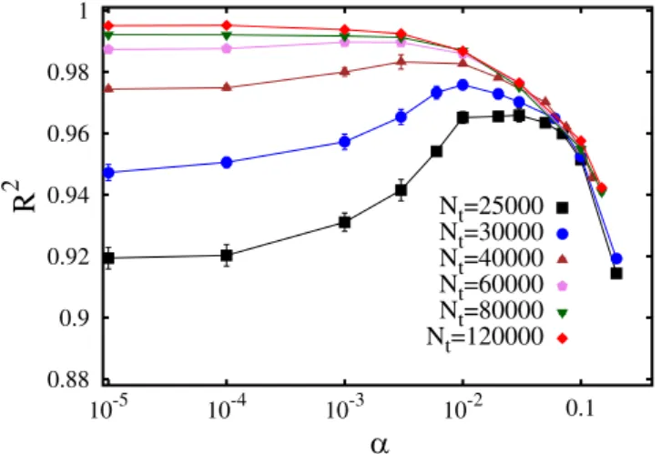
The first aspect of the machine learning process we analyze is the role of the regularization parameter α. A neural network with Nl = 3 hidden layers and Nn = 150 neurons per hidden layer is considered for this analysis, testing how accurately it predicts the (shifted) ground state energies of the Np = 40000 instances of the test set. Figure 4 shows the R2 scores as a function of the regularization parameter, for different sizes of the training set N
t. One notices that for the smallest training set with Nt = 25000 instances the optimal result is obtained with a sig-nificantly large regularization parameter, namely α ≈ 0.03. This indicates that without regularization this training set would be too small to avoid overfitting. Instead, the largest training sets provide the highest R2 scores with vanishingly small α values, meaning that here regularization can be avoided. In fact, this neural network proves able to accurately predict the ground-state energies of the speckle-field instances, with the highest values of the coefficient of determination R2 close to 1.
This high accuracy can be appreciated also in the scatter plot of Fig. 5, where the shifted ground-state energy
εpred = F(f) predicted by the neural network (with N
l = 3 and Nn = 150, as in Fig. 4) is plotted versus the exact value ε0. Here, the training set size is Nt = 80000, and the regularization parameter is fixed at the optimal value. The color scale indicates the absolute value of the discrepancy d = εpred − ε
0. One notices that somewhat larger dis-crepancies occur for those speckle-field instances whose ground state energy is higher than the average. The inset of Fig. 5 displays its probability distribution P(d). This distribution turns out to be well described by a gaussian fitting function with a standard deviation as small as σ ≅ 0.039Ec.
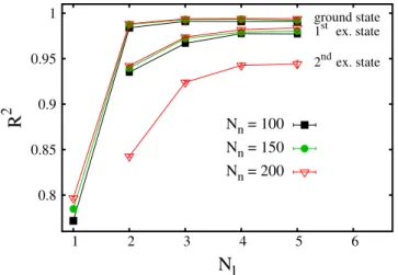
It is interesting to analyze how the accuracy of the neural network varies with the number of hidden layers
Nl and of the neuron per hidden layer Nn. In Fig. 6 the R2 scores are plotted as a function of Nl. The three upper datasets correspond to (shifted) ground-state energy predictions with three values of Nn. In Fig. 7 the R2 scores are plotted as a function of Nn, for three numbers of layers Nl. The size of the training set is Nt = 80000. One notices
that a neural network with only one hidden layer is not particularly accurate, with the R2 score being close to
R2 ≈ 0.8. Instead, two hidden layers appear to be already sufficient to provide accurate predictions. Increasing the hidden layer number beyond Nl = 3 does not provide a sizable accuracy improvement. The number of neurons
Nn plays a relevant role, too. A significant accuracy improvement occurs when the number of hidden neurons increases from Nn = 50 to Nn = 100. This improvement becomes less pronounced when Nn is increased beyond
Nn = 150.
It is evident that neural networks with Nl > 2 and Nn > 150 are quite accurate statistical models to predict ground state energies; however, their R2 scores still remain close but systematically below the ideal result R2 = 1. It is possible that a larger training set would allow one to remove even this small residual error. To address this point, we plot in Fig. 8 the gap with respect to the ideal score, computed as 1 − R2, as a function of the training set size Nt, reaching relatively large training set sizes Nt = 140000. The considered neural network is considerably deep and wide, having Nl = 3 hidden layers and Nn = 200 neurons per hidden layer. One observes that this gap systematically decreases with Nt. In fact, for ≥Nt 50000, the gap data trend appears to be reasonably well
charac-terized by the following power-law fitting function: 1 − R2(N
t) = A/Nt, where A = 513(6) is the only fitting param-eter. We emphasize here that this fitting function is empirical, that it applies to the considered regime of large training set sizes Nt, and that is is possible that the gap data would display a different scaling (e.g., logarithmically vanishing) for even larger Nt values. Still, the analysis of Fig. 8 suggests that, given a sufficiently large training set, a few-layers deep neural network can provide essentially arbitrarily accurate predictions of ground-state energies. Chiefly, one notices that at Nt = 140000 the R2 score is as accurate as R2 ≅ 0.996, meaning that the residual error is already negligible for many purposes. The training process of a deep neural network on much larger training sets
0.88 0.9 0.92 0.94 0.96 0.98 1 10-5 10-4 10-3 10-2 0.1
R
2α
Nt=25000 Nt=30000 Nt=40000 Nt=60000 Nt=80000 Nt=120000Figure 4. Coefficient of determination R2 as a function of the regularization parameter α. The different datasets correspond to different training set sizes Nt. The neural network has Nl = 3 layers and Nn = 150 neurons per layer. -1.5 -1 -0.5 0 0.5 1 1.5 2 -1.5 -1 -0.5 0 0.5 1 1.5 2
ε
predε
0 0 0.05 0.1 0.15 0.2 0.25 0 2 4 6 8 10 -0.2 0 0.2 d P(d)Figure 5. Main panel: shifted energy levels predicted by the neural network εpred as a function of the (shifted) exact values ε0 determined via the finite difference technique. The color scale indicates the absolute value of the discrepancy d = εpred − ε0. Inset: probability distribution of the discrepancy d. The (green) continuous curve is a Gaussian fitting function = − σ
π σ
P d( ) 21 exp[ d2/(2 )]2 , with the fitting parameter σ ≅ 0.039E
0.8 0.85 0.9 0.95 1 1 2 3 4 5 6 ground state 1st ex. state 2ndex. state
R
2N
l Nn = 100 Nn = 150 Nn = 200Figure 6. Coefficient of determination R2 as a function of the number of layers N
l of the neural network. The upper three datasets correspond to the ground-state energy level, for three numbers of neuron per layer Nn. The central three datasets correspond to the first excited state. The lowest dataset corresponds to the second excited state. 0.965 0.97 0.975 0.98 0.985 0.99 0.995 1 50 100 150 200 250
R
2N
n Nl = 2 Nl = 3 Nl = 4Figure 7. Coefficient of determination R2 for the prediction of ground state energy levels, as a function of the number of neurons per layer Nn. The three datasets correspond to different numbers of layers Nl.
0.004 0.008 0.016 40000 60000 90000 135000
1 -
R
2N
tFigure 8. Difference between the ideal value of the coefficient of determination R2 = 1 and the actual R2-score obtained in the prediction of ground state energy levels, as a function of the training set size Nt. The (red) line is a power-law fitting function for ≥Nt 50000 of the type: 1 − R2(Nt) = A/Nt, with A a fitting parameter. The number of layers is Nl = 3 and the number of neurons per layer is Nn = 200.
becomes a computationally expensive task, at the limit of the computational resources available to us. In this regards, it is worth reminding that the computational cost of training a neural network scales with the training set size, with the number of features, and with the Nl-th power of the number of neurons per hidden layer. In fact, in general, the inaccuracies in supervised machine learning predictions can be attributed to the limited expressive power of the statistical model (e.g., an artificial neural network with too few hidden layers), but also to the possi-ble inability of the training algorithm to find the optimal parameters. In the case analyzed here, it appears that the training algorithm is not the limiting factor, since the R2 scores systematically improve with N
t. However, substan-tial research efforts are still being devoted to improve the power and the speed of the optimization algorithms employed to train artificial neural networks, and even quantum annealing methods have recently been tested60.
We analyze also how accurately a neural network can predict the (shifted) excited state energies. In fact, in quantum many-body theory, predicting excited state energies is a more challenging computational problem com-pared to ground-state energy computations, since efficient numerical algorithms such as, e.g., quantum Monte Carlo simulations, cannot be used in general, thus demanding the use of computationally expensive techniques like exact diagonalization algorithms. It is interesting to inspect if this greater difficulty is reflected in the process of learning to predict excited state energies from previous observations. R2 scores corresponding to predictions of first excited state energies are displayed in Fig. 6, as a function of Nl, for three numbers of neurons per hidden layer Nn. R2 scores corresponding to the second excited state are displayed too, but for one Nn value only. One notices that the R2 scores are lower than in the case of ground state energy predictions, in particular the results corresponding to the second excited state. Furthermore, the number of layers appears to play a more relevant role. Deeper neural networks are necessary to get close to the ideal score R2 = 1. However, adding even more layers becomes computationally prohibitive, and is beyond the scope of this article.
It is worth mentioning that machine learning techniques have been recently employed to develop compact representations of many-body wave functions of tight-binding and quantum spin models. In particular, a specific kind of generative (shallow) neural network, namely the restricted Boltzmann machine, has been found to be capable of accurately approximating ground-state wave functions61. Unrestricted Boltzmann machines, including direct correlations among hidden variables, have been considered, too62. Interestingly, it was later found that in order to accurately represent (low-lying) excited states, deeper neural networks are required63, in line with our findings on energy-level approximation.
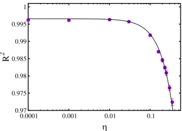
The last aspect we investigate is the resilience of the neural network to the noise eventually present in the data representing the energy levels of the training set. Quantifying this (possible) resilience is important in order to establish if it is feasible to employ the outcomes of analog quantum simulations performed, e.g., with ultracold atom experiments, to train neural networks. In fact, while training sets obtained from numerical computations, as the exact diagonalization calculation employed here, are in general free from random fluctuations (this is not the case, e.g., of Monte Carlo simulations), in experiments a certain amount of statistical uncertainty is unavoidable. With this aim, we perform the training of a neural network on a large set of instances whose (shifted) energy lev-els εi have been randomly distorted by adding a Gaussian random variable with zero mean and standard deviation equal to the standard deviation of the original set of energy levels times a scale factor η. This scale factor quan-tifies the intensity of the noise added to the training set. Specifically, we consider a neural network with Nl = 3 layers, Nn = 200 neurons per layer, while the size of the training set is the largest considered in this article, namely
Nt = 140000. The results for the coefficient of determination R2 (computed on Np non-randomized test instances, previously unseen by the neural network) as a function of the noise intensity η are shown in Fig. 9. One notices
0.97 0.975 0.98 0.985 0.99 0.995 1 0.0001 0.001 0.01 0.1
R
2η
Figure 9. Coefficient of determination R2 for the prediction of ground state energy levels as a function of the amount of noise added to the training set. The noise is introduced by adding to the (shifted) energy levels Gaussian random variables with zero mean and standard deviation equal to the standard deviation of the energy levels of the training set times the noise-intensity parameter η. The (back) curve is an empirical fitting function of the type: R2(η) = a − bηc, with fitting parameters a = 0.9966(2), b = 0.11(1), and c = 1.38(7). The number of layers of the neural network is Nl = 3, the number of neurons per layer is Nn = 200, while the training set size is
that the prediction accuracy is essentially unaffected by the added noise up to a noise level of a few percent. Only when the noise level is above 10% (corresponding to η > 0.1) the reduction in the R2 score becomes significant. The R2 data appear to be well described by the empirical fitting function R2(η) = a − bηc, with a, b, and c fitting parameters. These results indicate that the neural network is capable of filtering out the signal from the noise, resulting in a remarkable resilience to the random noise present in the training set. It is worth mentioning that, analogously to the analyses reported above, the regularization parameter α has been optimized for each η value, individually. These optimizations show that, while for small added noise (small η) vanishingly small α values are optimal, meaning that no regularization is needed, larger α values are need when the noise intensity increases; for example, when η = 0.35 the optimal regularization parameter (the one providing the highest R2 score on the test set) is α = 0.01. This indicates that, by penalizing models with large weight coefficients, the regularization helps the neural network to avoid learning the noise, thus filtering out the signal.
These findings suggest that data obtained from cold-atom quantum simulations might be used to train neural network, possibly providing a route to make predictions on models that cannot be accurately solved via computer simulations, as for the paradigmatic case of the fermionic Hubbard model. Concerning this, it is worth men-tioning that recent cold-atoms experiments implementing the fermionic Hubbard model have been analyzed via machine learning techniques38, and we hope that our findings will motivate further endeavours in this direction. It is also worth mentioning that previous studies on classification problems via supervised machine learning have already found that deep neural networks are remarkably robust against noise; see, e.g., ref.64 and references there in. In those studies, noise was introduced in the form of many instances with random labels, even at the point of outnumbering the instances with correct labels. Our results extend these previous findings to the case of a specific, experimentally relevant, regression problem. It is also worth pointing out that techniques to reduce the effect of random errors in the training set have been developed in the machine learning community (see, e.g. ref.65), and that such techniques could be adapted to analyze cold-atom experiments.
Discussion
The general problem we tried to address is whether a machine can learn to solve new quantum mechanics prob-lems from previously solved examples. Specifically, we performed a supervised machine learning study, training a deep neural network to predict the lowest three energy levels of a quantum particle in a disordered external field. The trained neural network could be employed, e.g., to speed up the ensemble averaging calculations, for which numerous realizations have to be considered in order to faithfully represent the disorder ensemble. This kind of ensemble averaging plays a crucial role in the studies on Anderson localization (see, e.g, refs49,50). The quantum model we focused on is designed to describe a one-dimensional noninteracting atomic gas exposed to an optical speckle field, taking into account the structure of the spatial correlations of the local intensities of the random field. The most relevant aspects of a supervised machine learning task have been analyzed, including the number of hidden layers in the neural network, the number of neurons in each hidden layer, the size of the training set, and the magnitude of the regularization parameter. Interestingly, we found that a neural network with three or four layers of hidden neurons can provide extremely accurate prediction of ground-state energies using for training a computationally feasible number of speckle-field instances. The predictions of excited state energies turned out to be slightly less accurate, requiring deeper neural networks to approach the optimal result. We also quantified the amount of regularization required to avoid the overfitting problem in the case of small or moderately large training sets.
In recent years, the experiments performed with ultracold atoms have emerged as an ideal platform to per-form quantum simulations of complex quantum phenomena observed also in other, less accessible and less tun-able, condensed matter systems. In the long term, one can envision the use of cold-atom setups to train artificial neural network to solve problems that challenge many-body theorists, like the many-fermion problem. In the medium term, these experiments can be employed as a testbed to develop efficient representations of instances of quantum systems for supervised machine learning tasks, as well as for testing the accuracy of different statis-tical models, including, e.g, artificial neural networks, convolutional neural networks, gaussian approximation potentials, or support vector machines19,24. These machine learning techniques could find use in particular in the determination of potential energy surfaces for electronic structure simulations29, or even in ligand-protein affinity calculations for drug-design research. For this purpose, it is of outmost importance to understand how accurate the above mentioned statistical models can be in predicting the energy levels of complex quantum many body systems. This is one of the reasons that motivated our study. In view of the possible future use of cold-atom quantum simulators as computational engines to provide training sets for supervised machine learning tasks, we investigated the resilience of artificial neural networks to noise in the training data, since this is always present is any experimental result. We found that a deep neural network with three layers is remarkably robust to such noise, even up to a 10% noise level in the target values of the training data. This level of accuracy is indeed within the reach of cold-atoms experiments. This is an important result suggesting that training artificial neural net-works using data obtained from cold-atom quantum simulations would indeed be feasible. The analysis on the amount of regularization discussed above provides information on how many experimental measurements would be needed to avoid the risk of overfitting.
It well known that an accurate selection of the features used to represent the system instances can greatly enhance the power of supervised machine learning approaches. In this article we have employed the Fourier com-ponents of the optical speckle field. This appears to be an effective choice for systems characterized by external fields with spatial correlations. This approach could be further improved by combining this choice of features with different types of artificial neural networks as, e.g., the convolutional neural networks; the latter have in fact been considered in ref.19, but in combination with a real-space representation of the quantum system. In this regards, it is worth mentioning that various alternative representations have been considered in the field of atomistic simu-lations for many-particle systems, including, e.g, the atom-centered symmetry functions26, the neighbor density,
the smooth overlap of atomic positions, the Coulomb matrices (see, e.g, ref.29), and the bag of bonds model13. In this context, an important open problem is the development of space-scalable representations, and associated statistical models, that can be applied to systems of increasing system size. Previous machine-learning studies on atomistic systems exploited the locality of atomic interaction to build such scalable models for many-atom sys-tems22,29. This property, which is sometimes referred to as nearsightedness, characterizes many common chemical systems. However, quantum mechanical systems often host long-range correlations that cannot be captured by locality-based models. A more general approach, which will be the focus of future investigations, might be built using transfer-learning techniques66 whereby models optimized on small scale systems form the building blocks of neural-network models for large scale systems with a moderate computational cost.
Data Availability
All data sets and computer codes employed in this work are available upon request.
References
1. Snyder, J. C., Rupp, M., Hansen, K., Müller, K.-R. & Burke, K. Finding density functionals with machine learning. Phys. Rev. Lett.
108, 253002 (2012).
2. Li, L. et al. Understanding machine-learned density functionals. Int. J. Quantum Chem. 116, 819–833 (2016). 3. Brockherde, F. et al. Bypassing the Kohn-Sham equations with machine learning. Nat. Commun. 8, 872 (2017). 4. Snyder, J. C. et al. Orbital-free bond breaking via machine learning. J. Chem Phys. 139, 224104 (2013). 5. Wang, L. Discovering phase transitions with unsupervised learning. Phys. Rev. B 94, 195105 (2016). 6. Carrasquilla, J. & Melko, R. G. Machine learning phases of matter. Nat. Phys. 13, 431 (2017).
7. Van Nieuwenburg, E. P., Liu, Y.-H. & Huber, S. D. Learning phase transitions by confusion. Nat. Phys. 13, 435 (2017).
8. Ch’ng, K., Carrasquilla, J., Melko, R. G. & Khatami, E. Machine learning phases of strongly correlated fermions. Phys. Rev. X 7, 031038 (2017).
9. Wetzel, S. J. Unsupervised learning of phase transitions: From principal component analysis to variational autoencoders. Phys. Rev.
E 96, 022140 (2017).
10. Deng, D.-L., Li, X. & Sarma, S. D. Machine learning topological states. Phys. Rev. B 96, 195145 (2017).
11. Ohtsuki, T. & Ohtsuki, T. Deep learning the quantum phase transitions in random electron systems: Applications to three dimensions. Jour. Phys. Soc. Jap. 86, 044708 (2017).
12. Hansen, K. et al. Assessment and validation of machine learning methods for predicting molecular atomization energies. J. Chem.
Theory Comput. 9, 3404–3419 (2013).
13. Hansen, K. et al. Machine learning predictions of molecular properties: Accurate many-body potentials and nonlocality in chemical space. J. Phys. Chem. Lett. 6, 2326–2331 (2015).
14. Schütt, K. et al. How to represent crystal structures for machine learning: Towards fast prediction of electronic properties. Phys. Rev.
B 89, 205118 (2014).
15. Ragoza, M., Hochuli, J., Idrobo, E., Sunseri, J. & Koes, D. R. Protein–ligand scoring with convolutional neural networks. J. Chem. Inf.
Model. 57, 942–957 (2017).
16. Wójcikowski, M., Ballester, P. J. & Siedlecki, P. Performance of machine-learning scoring functions in structure-based virtual screening. Sci. Rep. 7, 46710 (2017).
17. Khamis, M. A., Gomaa, W. & Ahmed, W. F. Machine learning in computational docking. Artif. Intell. Med. 63, 135–152 (2015). 18. Pereira, J. C., Caffarena, E. R. & dos Santos, C. N. Boosting docking-based virtual screening with deep learning. J. Chem. Inf. Model.
56, 2495–2506 (2016).
19. Mills, K., Spanner, M. & Tamblyn, I. Deep learning and the Schrödinger equation. Phys. Rev. A 96, 042113 (2017).
20. Blank, T. B., Brown, S. D., Calhoun, A. W. & Doren, D. J. Neural network models of potential energy surfaces. J. Chem. Phys. 103, 4129–4137 (1995).
21. Lorenz, S., Groß, A. & Scheffler, M. Representing high-dimensional potential-energy surfaces for reactions at surfaces by neural networks. Chem. Phys. Lett. 395, 210–215 (2004).
22. Behler, J. & Parrinello, M. Generalized neural-network representation of high-dimensional potential-energy surfaces. Phys. Rev.
Lett. 98, 146401 (2007).
23. Handley, C. M. & Popelier, P. L. Potential energy surfaces fitted by artificial neural networks. J. Phys. Chem. A 114, 3371–3383 (2010).
24. Bartók, A. P., Payne, M. C., Kondor, R. & Csányi, G. Gaussian approximation potentials: The accuracy of quantum mechanics, without the electrons. Phys. Rev. Lett. 104, 136403 (2010).
25. Behler, J. Neural network potential-energy surfaces in chemistry: a tool for large-scale simulations. Phys. Chem. Chem. Phys. 13, 17930–17955 (2011).
26. Behler, J. Atom-centered symmetry functions for constructing high-dimensional neural network potentials. J. Chem. Phys. 134, 074106 (2011).
27. Cheng, B., Engel, E. A., Behler, J., Dellago, C. & Ceriotti, M. Ab initio thermodynamics of liquid and solid water. arXiv preprint
arXiv:1811.08630 (2018).
28. LeCun, Y., Bengio, Y. & Hinton, G. Deep learning. Nat. 521, 436 (2015).
29. Behler, J. Perspective: Machine learning potentials for atomistic simulations. J. Chem. Phys. 145, 170901 (2016).
30. Schütt, K. T., Arbabzadah, F., Chmiela, S., Müller, K. R. & Tkatchenko, A. Quantum-chemical insights from deep tensor neural networks. Nat. Commun. 8, 13890 (2017).
31. Giorgini, S., Pitaevskii, L. P. & Stringari, S. Theory of ultracold atomic Fermi gases. Rev. Mod. Phys. 80, 1215 (2008). 32. Bloch, I., Dalibard, J. & Zwerger, W. Many-body physics with ultracold gases. Rev. Mod. Phys. 80, 885 (2008). 33. Jaksch, D. & Zoller, P. The cold atom Hubbard toolbox. Ann. Phys. 315, 52–79 (2005).
34. Bernien, H. et al. Probing many-body dynamics on a 51-atom quantum simulator. Nat. 551, 579 (2017).
35. Hart, R. A. et al. Observation of antiferromagnetic correlations in the hubbard model with ultracold atoms. Nat. 519, 211 (2015). 36. Cheuk, L. W. et al. Observation of spatial charge and spin correlations in the 2d fermi-hubbard model. Sci. 353, 1260–1264 (2016). 37. Mazurenko, A. et al. A cold-atom fermi–hubbard antiferromagnet. Nat. 545, 462 (2017).
38. Bohrdt, A. et al. Classifying snapshots of the doped hubbard model with machine learning. arXiv preprint arXiv:1811.12425 (2018). 39. Roati, G. et al. Anderson localization of a non-interacting Bose–Einstein condensate. Nat. 453, 895–898 (2008).
40. Billy, J. et al. Direct observation of Anderson localization of matter waves in a controlled disorder. Nat. 453, 891–894 (2008). 41. Aspect, A. & Inguscio, M. Anderson localization of ultracold atoms. Phys. Today 62, 30–35 (2009).
42. Kondov, S., McGehee, W., Zirbel, J. & DeMarco, B. Three-dimensional Anderson localization of ultracold matter. Sci. 334, 66–68 (2011).
43. Jendrzejewski, F. et al. Three-dimensional localization of ultracold atoms in an optical disordered potential. Nat. Phys. 8, 398–403 (2012).
45. Goodman, J. W. Statistical properties of laser speckle patterns. In Laser speckle and related phenomena, 9–75 (Springer, 1975). 46. Goodman, J. W. Speckle phenomena in optics: theory and applications (Roberts and Company Publishers, 2007).
47. Falco, G., Fedorenko, A. A., Giacomelli, J. & Modugno, M. Density of states in an optical speckle potential. Phys. Rev. A 82, 053405 (2010).
48. Modugno, G. Anderson localization in Bose–Einstein condensates. Rep. Prog. Phys. 73, 102401 (2010).
49. Delande, D. & Orso, G. Mobility edge for cold atoms in laser speckle potentials. Phys. Rev. Lett. 113, 060601 (2014). 50. Fratini, E. & Pilati, S. Anderson localization of matter waves in quantum-chaos theory. Phys. Rev. A 91, 061601 (2015). 51. Fratini, E. & Pilati, S. Anderson localization in optical lattices with correlated disorder. Phys. Rev. A 92, 063621 (2015).
52. Izrailev, F. M. & Krokhin, A. A. Localization and the mobility edge in one-dimensional potentials with correlated disorder. Phys. Rev.
Lett. 82, 4062–4065 (1999).
53. Sanchez-Palencia, L. et al. Anderson localization of expanding Bose-Einstein condensates in random potentials. Phys. Rev. Lett. 98, 210401 (2007).
54. Lugan, P. et al. One-dimensional Anderson localization in certain correlated random potentials. Phys. Rev. A 80, 023605 (2009). 55. Huntley, J. Speckle photography fringe analysis: assessment of current algorithms. Appl. Opt. 28, 4316–4322 (1989).
56. Abrahams, E., Anderson, P. W., Licciardello, D. C. & Ramakrishnan, T. V. Scaling theory of localization: Absence of quantum diffusion in two dimensions. Phys. Rev. Lett. 42, 673–676 (1979).
57. Prat, T., Cherroret, N. & Delande, D. Semiclassical spectral function and density of states in speckle potentials. Phys. Rev. A 94, 022114 (2016).
58. Pedregosa, F. et al. Scikit-learn: Machine learning in Python. J. Mach. Learn. Res. 12, 2825–2830 (2011). 59. Kingma, D. P. & Ba, J. Adam: A method for stochastic optimization 1412.6980 (2014).
60. Baldassi, C. & Zecchina, R. Efficiency of quantum vs. classical annealing in nonconvex learning problems. Proc. Natl. Acad. Sci. USA 201711456 (2018).
61. Carleo, G. & Troyer, M. Solving the quantum many-body problem with artificial neural networks. Sci. 355, 602–606 (2017). 62. Inack, E. M., Santoro, G. E., Dell’Anna, L. & Pilati, S. Projective quantum Monte Carlo simulations guided by unrestricted neural
network states. Phys. Rev. B 98, 235145 (2018).
63. Choo, K., Carleo, G., Regnault, N. & Neupert, T. Symmetries and many-body excited states with neural-network quantum states.
arXiv preprint arXiv:1807.03325 (2018).
64. Rolnick, D., Veit, A., Belongie, S. & Shavit, N. Deep learning is robust to massive label noise (2018).
65. Reed, S. et al. Training deep neural networks on noisy labels with bootstrapping. arXiv preprint arXiv:1412.6596 (2014). 66. Pan, S. J. et al. A survey on transfer learning. IEEE Transactions on knowledge data engineering 22, 1345–1359 (2010).
Acknowledgements
We acknowledge insightful discussions with Andrea De Simone and Giuseppe Carleo. S.P. acknowledges the CINECA award under the ISCRA initiative, for the availability of high performance computing resources and support. Partial support by the Italian MIUR under PRIN-2015 Contract No. 2015C5SEJJ001 is also acknowledged.
Author Contributions
S. Pilati and P. Pieri conceived the project and wrote the manuscript. S. Pilati performed the computations.
Additional Information
Competing Interests: The authors declare no competing interests.
Publisher’s note: Springer Nature remains neutral with regard to jurisdictional claims in published maps and
institutional affiliations.
Open Access This article is licensed under a Creative Commons Attribution 4.0 International
License, which permits use, sharing, adaptation, distribution and reproduction in any medium or format, as long as you give appropriate credit to the original author(s) and the source, provide a link to the Cre-ative Commons license, and indicate if changes were made. The images or other third party material in this article are included in the article’s Creative Commons license, unless indicated otherwise in a credit line to the material. If material is not included in the article’s Creative Commons license and your intended use is not per-mitted by statutory regulation or exceeds the perper-mitted use, you will need to obtain permission directly from the copyright holder. To view a copy of this license, visit http://creativecommons.org/licenses/by/4.0/.