In the course of this thesis the B-spline K-matrix method, a theoretical technique capable of reproducing the single ionization continuum of atoms, was developed. Two systems were addressed in particular: helium and boron, as representatives of two- and three-active-electron atoms.
Some of the findings presented here resulted in original contributions to the sci-entific literature. Total and partial photoionization cross sections and asymmetry parameters of the fundamental helium state were examined up to the sixth ioniza-tion threshold, yielding the first ab initio reproducioniza-tion of the first intruder state effects below N=4 threshold, the first reproduction of dipole asymmetry param-eters below N=6 threshold and of nondipole anisotropy parameter γ below N=2 threshold.
Most of the material presented here relies on the multiple basis implementa-tion of the B-spline K-matrix method which allows the reproducimplementa-tion of almost arbitrarily excited metastable satellites below a prescribed threshold. The new technique, when used to investigate helium triplet states, yielded the most accu-rate and extensive existing characterization of triplet metastable states up to the fifth ionization threshold. Within more than 1700 natural and unnatural S, P and D doubly excited states, eleven intruder states were discovered, entirely unknown before.
At least two experimental groups, at ELETTRA in Trieste and at BESSY II in Berlin, are recently tackling the problem of measuring the metastable 23S helium
photoionization cross section. We therefore undertook a parallel theoretical inves-tigation of the photoionization process of both the fundamental and the excited3S
helium states. The latter prelude to the future investigation of the radiative decay of doubly excited states and already revealed interesting peculiar features.
To this purpose, we devised an extension of the K-matrix method to treat the atom-radiation interaction non perturbatively.
A general three electron package has been developed and applied to study boron resonances. Specific formulas were derived to obtain arbitrary tensorial one-particle and scalar two-one-particle matrix elements between three electron states on non-orthogonal basis as required for an efficient exploitation of B-splines.
A detailed study of the B-spline effective completeness led to a general result which assure that B-spline based methods are well conditioned for a large class of knot grids.
1.5 Basis Conditioning . . . 19 1.6 B-splines . . . 22 1.6.1 Flexibility . . . 22 1.6.2 Efficiency . . . 24 1.7 Resonance characterization . . . 27 1.8 Radiative K-matrix . . . 30
2 Singlet helium photoionization 33 2.1 Introduction . . . 33
2.2 [031]+5, the first intruder state . . . 34
2.3 Below N=5 threshold . . . 42
2.4 Below N=6 threshold . . . 46
2.5 Non dipole effects . . . 48
3 Helium triplet states 55 3.1 Introduction . . . 55
3.2 Autoionization decay paths . . . 57
3.3 Computational details . . . 60 3.4 Below N=1 threshold. . . 62 3.5 Below N=2 threshold. . . 64 3.6 Below N=3 threshold. . . 74 3.7 Below N=4 threshold. . . 82 3.8 Below N=5 threshold. . . 89 3.9 Intruder states . . . 94
3.10 Photoionization of Rydberg satellites . . . 99
3.11 Radiative decay of doubly excited states . . . 101
4 Three electron systems 104 4.1 Separation of spin and spatial components . . . 104
4.3 Boron . . . 106
4.3.1 Polarizable core . . . 107
A Scattering 121 A.1 Time dependent theory . . . 121
A.2 Time independent theory . . . 124
A.3 Transition rate . . . 126
A.4 Scattering cross section . . . 128
A.5 Partial wave expansion . . . 128
B Atom-radiation interaction 131 B.1 Field quantization . . . 131
B.2 Transition amplitudes and rates . . . 138
B.3 Driven Schr¨odinger equation . . . 139
B.4 Multipolar expansion . . . 139
B.5 Expansion of the outgoing electron wave . . . 143
B.6 Orientational Average . . . 144
B.7 Integral cross sections . . . 145
B.8 Dipole anisotropy parameter β . . . 146
B.9 Beyond the dipole approximation . . . 149
B.9.1 E1-E2 . . . 150
B.9.2 E1-M1 . . . 154
B.10 Radiative decay . . . 156
B.11 Radiative transitions in the continuum . . . 156
B.12 Gauges . . . 161
C B-Splines 163 C.1 Definition and basic properties . . . 163
C.2 Free knots optimization . . . 166
C.3 Effective completeness . . . 170
C.4 Locally uniform grids and locally Toeplitz matrices . . . 180
C.5 Min-max theorem and its consequences . . . 180
C.5.1 Interlace theorem . . . 181
C.5.2 Finite rank perturbation . . . 181
C.5.3 Perturbations with small spectral radius . . . 182
D Interpolation 183 E Radiative K-matrix, an example 185 F Helium doubly excited states 190 G Matrix Elements 193 G.1 Graphical rules for angular momentum theory . . . 194
G.2 Single particle operators . . . 197
I Representation of effective potentials 217
J Boron Data Tables 231
K Energy levels, resonances and oscillator strengths in triplet He 240
Since Hertz’s discovery of the photoelectric effect in 1887 [1] and its proper expla-nation by Einstein in 1905 [2], photofragmentation processes proved to be among the most prolific means of investigation of atomic and molecular system dynamics. In 1928 Compton and Boyce [3], and Kruger [4], two years later, found in the arc spectrum of helium the first evidence of a doubly excited state, assigning the 320.392 ˚A line to the (2p2)3Pe→ (2s2p)3Po radiative decay.
The experimental practice made a considerable step forward when, in 1963, Madden and Codling [5] showed that synchrotron radiation is a useful X-ray source for spectroscopic purposes: they succeeded in measuring the first reso-nant profile in the photoionization spectrum of helium. Dedicated beamlines for atomic and molecular photoelectron spectroscopy experiments are now available at synchrotron laboratories all around the world: the Advanced Light Source at Berkeley [6], ELETTRA ring in Trieste [7], BESSY II in Berlin [8], Photon Fac-tory in Tsukuba [9], SOLEIL near Paris [10], the Advanced Photon Source near Chicago [11], Synchrotron Radiation Source at Daresbury [12] and Max-Lab in Lund [13], just to mention the most relevant.
Despite its simplicity, helium, the smallest atom with electronic correlation, has been one of the most studied systems because of its almost inexhaustible man-ifold phenomenology, progressively disclosing as new, more refined experimental techniques became available.
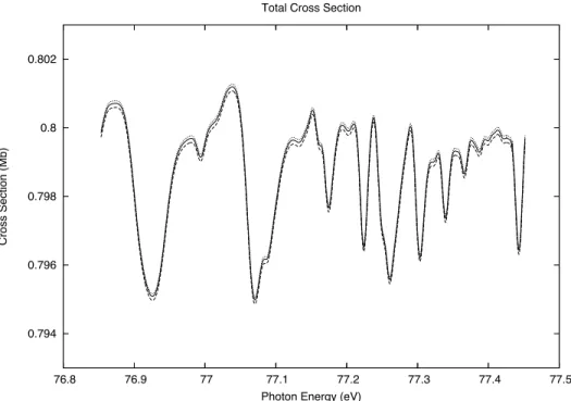
Many characteristic Fano profiles were already clearly visible in the total pho-toionization cross section collected in 1963 by Madden and Codling [5]. Twenty years after, the first partial differential cross sections were measured [14] and, in the early nineties, the energy resolution dropped sharply through ∼ 5 meV [15] to∼ 2 meV [16] when Domke et al observed for the first time the elusive (2p, nd)
1Po autoionizing Rydberg series below N=2 threshold. In the same period, the
first detailed spectra of dipole anisotropy parameters also appeared [17]. By 1996, in new observations of helium doubly excited states, the unprecedented ∼ 1 meV resolution was achieved [18, 19].
At higher energies, the regular pattern of autoionizing multiplets were found to be perturbed by intruder states from series converging to high lying thresholds [20–22]. In the neighborhood of double photoionization threshold, myriad intruder states accumulates until roughly between N ∼ 8 and N ∼ 13 thresholds, any regularity is virtually lost [23–26]
tion. In 2000, Gorczyca et al [29] demonstrated that both radiative decay and spin-orbit interaction had to be considered to account for the observed features of the photoionization spectrum in the immediate neighborhood of N = 2 threshold. In 2001 Penent et al eventually observed the radiative decay of triplet doubly ex-cited states in the photoionization of the helium atom in its ground state [30]. The branching ratio between autoionization and radiative decay was measured only few years ago [31].
Measurements of photoionization spectra of metastable states are now afford-able: preliminary results on the first resonant features in 23S He spectrum have
recently been presented [32] and closer investigations are on schedule [33, 34]. Many new measurements on doubly excited states with symmetry which cannot be reached in ordinary photoionization experiments have recently been made acces-sible through the application of external electric [35–37] and magnetic fields [38,39]. Finally, sizable non dipole effects were found at unexpectedly low energies even in a target as small as helium [40].
All of these experimental findings represented in the past, and are often today, challenges to ever more accurate and reliable theories. The multiple basis B-spline K-matrix method developed in this thesis is one of them. It succeeded in providing original reproductions of some of the observations outlined above, often unveiling previously unknown details. Moreover, as discussed at length in the following chapters, it has unique features that makes it particularly fit to deal naturally with those processes which involves highly excited Rydberg series below prescribed thresholds, like the radiative cascades originating from doubly excited states.
B-spline K-matrix method
1.1
Outline of photoionization observables
In atomic photoionization experiments, the gaseous target is introduced through a thin nozzle into a vacuum chamber where it intersects a photon beam. Upon photon absorption, the atom generally undergoes manifold transformations where two or more fragments, electrons, photons, ions, excited neutral states, result.
Let consider the exemplary case of helium in its fundamental state, illuminated with X-rays in the energy range between 24.6 eV and 79 eV, corresponding to single and double helium ionization thresholds respectively. With the absorption of one photon, helium may readily eject one electron (single photonionization - SPI), possibly leaving the parent ion in an excited state if Eγ > 65.4 eV (He+ excitation
threshold), or it may be temporarily trapped in a metastable state where, to a crude approximation, both the electrons are excited out of the fundamental level into outer bound orbitals (double photoexcitation - DPE). Such doubly excited states (DES) most often decay through autoionization (AI): one electron is eventually captured in a low-lying bound state of the parent ion releasing to the other electron enough energy to escape the atom. Since direct SPI and resonant AI result in the same final states, they give rise to characteristic interference figures in the photoionization spectra, known as Fano profiles [41].
If a metastable state is sufficiently long lived, the radiative decay (RD) may become a competitive or even dominant relaxation mechanism. The metastable state can even decay radiatively to a state of lower energy which itself lies in the continuum (radiative autoionization - RAI). In such case, one electron and one photon are ejected simultaneously.
He∗∗ RAI ! ! ! ! ! ! !!! ! ! ! ! AI "" RD ##He∗+ γ" He + γ SP I " " " " $$" " " " " DP E # # # # # %% # # # # # He+∗+ e−+ γ"" He+∗+ e−
0.5%, and almost arbitrary polarizations: linear with arbitrary tilt, circular and elliptical.
To measure the total photoionization cross section (TCS), it is sufficient to collect directly all the ions produced [42]. To obtain partial cross sections and angular distribution parameters, instead, the photoelectrons are collected by time-of-flight spectrometers [43] along specific directions with small angular acceptances, e.g. 3◦-6◦. If the photoelectron has left the parent ion in the state α, its energy is
found about Eγ−Eα, where the energy of the impinging photon is narrowly peaked
about Eγ. The ratio between the probability per unit of time that a photoelectron
with energy Eγ−Eαis collected along the direction Ω with a solid angle acceptance
dΩ, and the total numeral photon flux density Φγ, defines the differential partial
cross section dσα/dΩ dσα dΩ ≡ dP (Eγ− Eα) dtdΩΦγ . (1.1)
In order to compare with the experiment, we can use the quantum mechanical theoretical expression analogous to 1.1 provided by perturbation theory. To the lowest order, the partial differential photoionization cross section is proportional to the square module of the matrix element of a suitable transition operator between the initial and final state of the atom:
dσα dΩ = (2π)2 cωγ |%ψ − α#k|() · n ! i=1 ei#kγ·#ri(p i|φ0&|2. (1.2)
The initial state φ0 is clearly that of the target atom when injected into the
re-action chamber. From the discussion above it is clear that the final state lies in the continuum: the photoelectron is asymptotically free, therefore its kinetic en-ergy may vary by arbitrarily small amounts. Since all the measuring devices are macroscopic, they select a final state which is a broad, almost monochromatic pho-toelectron wavepacket, times a parent ion state in a definite energy level α, and which may be approximated, in a time independent approach, with a plane wave (actually a Coulomb wave) for the photoelectron, suitably coupled to the parent ion in the state α, plus a linear combination of incoming spherical waves in all the degenerate channels (incoming boundary conditions). Such states, indicated with the symbol ψα#k− (α collects all the quantum numbers beyond the asymptotic photoelectron linear momentum, included the photoelectron spin projection), are also said to be controlled in the future: in a time dependent approach, any L2
indeed a nonvanishing component in channel α only, since after leaving the atom, the photoelectron wavepacket eventually is an outgoing wave.
In the photoionization of strongly localized states at energies up to few hundreds eV, the exponential factor in equation 1.2 may be confidently approximated with 1 (dipole approximation). In this case the transition operator is a true rank one tensor. As a consequence the well known dipole selection rules apply and only a small number of final continuum manifolds with definite symmetry need to be calculated. Moreover, when the parent ion orientation is not measured, the angular distribution of the photoelectron is entirely described with a single parameter, βα(E), ranging from−1 to 2:
dσα#k dΩ = σα(E) 4π " 1 + βα· 3 cos2θ− 1 2 # (1.3) where σα(E) is the integral cross section for channel alpha (see appendix B for the
definition of symbols) σα(E) = π 3 c ωγ(2L0+ 1) ! L$α $ $ $%φ0' ˆV10'ψ−ΓαE$α& $ $ $ 2 . (1.4)
For linearly polarized radiation, θ is the angle between the electron linear momen-tum and the light polarization axis. For circularly polarized radiation, equation 1.3 still holds, but θ is the angle between the electron and photon linear momenta. The expression of β for linearly polarized light is
βα = % ! LL! ! $α$!α √ 30Π$αLL!C $! α0 $α0 20(−) Lα+$α+L+L!+L0 & L" 2 L ,α Lα ,"α ' & 1 2 1 L" L0 L ' × × %φ0' ˆV10' ¯ψαE$(−)Γα&%φ0' ˆV 0 1' ¯ψ(−)Γ ! αE$! α& ∗ () % ! L$α $ $ $%φ0' ˆV10'ψαE$(−)Γα& $ $ $ 2( . (1.5)
As these formula shows, the theoretical reproduction of the experimentally ob-servable quantities can be reduced to the calculation of matrix elements between bound and continuum atomic states with definite spherical symmetry and fulfilling appropriate boundary conditions.
The theory of electromagnetic transitions, and the scattering theory needed to deal with atomic states in the continuum and to compute photoionization parame-ters is covered in detail in the appendices A and B. The present chapter describes how to obtain numerically the accurate atomic states in the continuum needed for a positive comparison with modern experiments.
1.2
The close coupling equations
The eigenfunction of a N +1-electron system at energies below the double ionization threshold, where at most one electron can leave the system, can be written as a
for the collection of spatial and spin variables for the first N electrons, and rN +1,
(rN +1and σN +1are the radius, direction and spin projection of the N +1-th electron.
The channel functions ¯ΦΓ
i are defined as parent ion (or atom) N-electron eigenstates
with well defined angular momentum, spin and parity, coupled with the N + 1-th electron spin-angular functions so to realize a specific total symmetry identified by parity, angular momentum, spin and their projections onto an axis, collectively indicated with Γ (we restrict the discussion to light systems, where the electrostatic approximation is justified - i.e. no magnetic interactions or other relativistic effects are taken into account). The χΓi’s are also referred to as pseudostate channel,
localized channel, or correlation functions.
At each energy E there are as many linearly independent solutions ΨΓ
j as the
number of ¯ΦΓ
i whose threshold Ej, the energy of the corresponding N-electron
bound state, is lower than E. The expansion coefficients bΓ
ij and the radial functions
FΓ
ij are such that ΨΓj is an eigenfunction of the total N-electron hamiltonian:
HΨΓ
j = EΨΓj. (1.7)
Equation 1.7 can be projected onto the χΓ
i, integrating over all the spin and radial
variables, and onto the ¯ΦΓ
j, integrating over all the variables except the N + 1-th
radius. The bΓ
ij are eventually eliminated, yielding a system of integrodifferential
equations known as the close coupling equations + −1 2 d2 dr2 + ,i(,i+ 1) 2r2 − Z − N r − )i , FijΓ(r)− − ! m & VimΓ(r)FmjΓ (r) + -. KimΓ (r, r") + XimΓ (r, r")/FmjΓ (r")dr" ' = 0 (1.8)
where ,i is the N + 1-th electron orbital angular momentum in the i-th channel
¯ ΦΓ
i, and )i = E− Ei is the asymptotic N + 1-th electron energy, negative for closed
channels, positive for open channels. VΓ
ij(r) is the local direct potential, while
KΓ
explicit expressions of these potentials are VijΓ(r, r") = N %¯ΦΓi| 1 rN N +1 − 1 rN +1|¯ ΦΓj&|r≡rN,r!≡rN+1 (1.9) KijΓ(r, r") = N %¯ΦΓi(XN−1, r"ΩNσN; ΩN +1σN +1)|(H − E) |¯ΦΓj(XN−1, rΩN +1σN +1; ΩNσN)& (1.10) XijΓ(r, r") = −N +1 N %¯Φ Γ
i|(H − E)Gχo(E; r, r")(H− E)|¯ΦΓj& (1.11)
where Gχo(E; r, r") =!
i
|χi&%χi|
E− Eiχ
To solve practical scattering or photoionization problems, the close coupling ex-pansion 1.6, which in principle lead to exact solutions, must be truncated to a finite set of channels ¯ΦΓ
i and correlation functions χΓi. Moreover, a prescription to get a
complete set of linearly independent solutions at each energy must be given, and these solutions must be labeled according to the boundary conditions they fulfill. Many techniques accomplishing these tasks in different ways have been proposed.
A class of methods, reviewed by Nesbet [44], define functionals of the FΓ
ij’s
which are stationary about the exact solutions satisfying prescribed asymptotic conditions [45,46]. Among these variational methods, Kohn’s [47] and Schwinger’s [48] are perhaps the most popular.
The most widely used technique in the late twenty years, the R-matrix method, was introduced by Wigner and Eisenbud [49–51] in connection to the study of nuclear reactions, but encountered a considerable success also in the atomic and molecular physics community. For a review of the R-matrix method applied to atomic and molecular scattering problems see [52].
In the R-matrix approach, the configuration space is partitioned into two re-gions, one where all the N + 1 electrons are confined within a prescribed radius a from the scattering centre, and one where only N electrons are confined within r < a, while rN +1> a. The boundary radius a must be chosen so that the nonlocal
exchange and correlation potential, which decay exponentially with r, are negli-gible, and the local direct potential has reached its asymptotic multipolar form. The close coupling expansion is truncated to a finite number of channels and the N-electron scatterer function and the N + 1-electron correlation functions are ex-panded on finite basis within ri < a. In this scheme, to any linear combination of
incoming N + 1-th electron wave components at the boundary r = a there corre-sponds a unique set of outgoing components which defines the scattering properties of the system within a. The effects of the inner region on the electron scattering are entirely defined through a suitable hermitian Green function whose spectral decomposition is obtained with a single diagonalization of the total hamiltonian restricted to the inner region, modified with the addition of the Bloch operator [53] (which restores the hamiltonian hermiticity, broken by the truncation of the space to a set of functions which do not vanish at the boundary). The diagonalization,
r → re . (1.12) The θ-independent (complex) eigenvalues of the scaled hamiltonian are directly the position of the system resonances. The complex scaling methods yielded initially unclear results because of the sensibility of observables upon the angle θ when the rotation was performed about the origin and basis functions with noncompact support were used. A significant improvement in the complex scaling technique was obtained with the introduction of exterior complex scaling (ECS) [55, 56], where the radius acquires a phase factor only after a prescribed boundary r0:
r→ rθ(r0− r) + [r0+ (r− r0)eıθ]θ(r− r0) (1.13)
With the inclusion of B-splines, ECS proved to be particularly successful not only in the characterization of metastable states [24] but more appealingly in yielding typical scattering observables like differential photoionization cross sections, not necessarily restricted only to single fragmentation processes. In 2004, Horner et al [57] obtained essentially exact results for the triply differential cross section of helium double photoionization. Today, ECS is among the most promising methods available.
The close coupling expansion 1.6 can be exploited directly in the solution of the time dependent Schr¨odinger equation [58]. In the case of photoionization the initial bound state is propagated under the influence of an external potential until the cross section can be extracted from the amplitude of the outgoing components of the wavefunction [59]. Smart implementations of such “brute force” methods seems to be the most appropriate to face the sophisticated photofragmentation processes made possible by today fs free electron laser facilities, but are clearly unfit to seek metastable states.
1.3
K-matrix
Formally a configuration interaction in the continuum, on the line of a pioneering paper by Fano [41], the L2 K-matrix method [60, 61] follows the close coupling
prescription: a complete set of stationary eigenfunctions of the hamiltonian ψPαE in the continuum, are approximated with a linear combination of partial wave channels φαE (PWC’s) plus a localized (or pseudostate) channel (LC):
ψPαE = φαE + ! γ ! -d) φγ' P E− )Kγ',αE (1.14)
where the index α runs over the open channels at energy E, while the index γ runs over all available channels (open and closed) including the LC.
Equation 1.14 echoes the Lippmann-Schwinger equation with the principal value Green function [62]
ψαEP = φαE + GPo(E)V ψPαE (1.15)
The Lippmann-Schwinger equation can indeed be cast in the form of equation 1.14, by defining the off-shell reaction matrix K as
Kγ',αE ≡ %φα'|V |ψPαE&. (1.16)
The converse is actually not true as the unperturbed channels φα' in 1.14 are
generally defined in such a way that they are not orthogonal. In particular they are not the eigenchannels of an unperturbed hermitian operator. This is not a problem as the 1.14 should simply be looked at as a configuration interaction expansion, where the EP−' factor allows Kγ',αE to be regular in the first continuous
energy index ), and this is all what is required in order to solve the problem with standard numerical techniques. Moreover, we shall see in the following that the on-shell K-matrix, as computed from 1.14, still is the Cayley transform of the true scattering matrix of the physical problem (App. A).
A PWC function is defined as an (N − 1)−electron bound parent state (atom or ion) ΦIα with well defined spin, parity, angular momentum and energy Iα ≡
(Sα, Πα, Lα, Eα), coupled to a single particle state with definite angular
momen-tum ,α and asymptotic energy ), to form an antisymmetric N electron state with
definite spin S, parity Π, angular momentum L and projections Σ and M, which we shall indicate with the collective index Γ≡ (S, Π, L, Σ, M):
φΓαE =A! σασ CSSΣασα1 2σ ! mαm CLLMαmα$αm Φσαmα Iα ⊗ 2ϕΓ,σm α . (1.17)
The radial parts of the one particle orbitals ϕΓ
α' are defined so that the φΓαE
diag-onalize the Hamiltonian within the (Γ, α) subspace: %φΓαEα+'| H |φ Γ αEα+'!& = (Eα+ )) δ()− ) "), ) > 0, (1.18) %φΓαEα+'i| H |φ Γ αEα+'j& = (Eα+ )i) δij, )i, )j < 0. (1.19)
The partial wave channels normalized as
%φαE|φαE!& = δ(E − E") (1.20)
have the following asymptotic behaviour φγE ∼ 0 2kγ π Φγ eiθγ(r)− e−iθγ(r) 2ikγr , θγ(r) = kγr +η log 2kγr−lγπ/2+σl+δl (1.21)
where Φγ is the parent ion function coupled to the spin and angular part of the
N + 1-th electron, kγ =
1
2(E− Eγ), η = Z/kγ, σl is the Coulomb phaseshift and
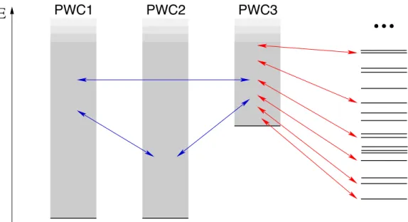
Figure 1.1: The K-matrix system of integral equations is a configuration interaction (CI) which includes the single ionization continuum. The set of continuum states in each partial wave channel is represented with a shadowed region above the channel threshold. The pile of levels on the right represent the pseudostate channel, comprising correlation functions as well as possible autoionizing states. All these channels interact with each other (arrows).
The localized channel comprises a large number of many-electron functions χΓ
i, with global symmetry Γ, built from localized orbitals, and which separately
diagonalizes the Hamiltonian:
%χΓi|χΓj& = δij, %χΓi|H|χΓj& = δijEiΓ, χΓi = ! j . 2 k ϕkj /Γ LS c i j (1.22)
Equation (1.14) may be solved for the off-shell reaction K-matrix functions by requiring ψαEP to be an eigenfunction of the complete projected hamiltonian with eigenvalue E:
%φβE!| E − H |ψPαE& = 0 ∀ β, E".
This leads to a system of integral equations for the off shell reaction matrix K: KβE!,αE −
!
γ'=β
!
-d) VβE!,γ'(E) P
E− )Kγ',αE = VβE!,αE(E)(1− δαβ) (1.23)
where the effective potential V is defined as
VβE!,αE ≡ %φβE| H − E |φαE& = HβE!,αE − E SβE!,αE
The K-matrix integral equations arise also in the minimization of a suitable func-tional through the Newton variafunc-tional principle [62]. At each energy, where the scattering space is n−fold degenerate, n linearly independent coupled-channel func-tions ψP
Consider now the following linear combinations of stationary wavefunctions ψ±E = ψPE[1± iπK(E)]−1
where ψ±E = (ψ±1E, . . . , ψ±nE) and Kα,β(E)≡ KαE,βE is known as on-shell reactance
matrix (see for example Newton §7.2.3 [62]). As r ≡ rN +1→ ∞
ψαE± ∼ open ! β 3 φβE+ open ! γ ! -d)φγ' P E− )Kγ',βE 4 [1± iπK(E)]−1βα = = φαE + open ! βγ ! -d)φγ' 1 E− ) ± i0+Kγ',βE[1± iπK(E)] −1 βα (1.24)
Replacing in the equation above the φγ' with their asymptotic behaviour 1.21, and
closing the integrals with suitable circuits in the complex k plane, the following expression is obtained ψαE± ∼ φαE− open ! γ 5 2π kγ Φγ e±iθγ(r) r 6 K(E) 1± iπK(E) 7 γα (1.25) In ψ±
α there are only outgoing (incoming) waves in all channels but α. In other
terms ψ± are recognized as the ordinary scattering solutions for wavepackets con-trolled in the past (future) (see appendix A). Since
%ψ±E|ψ±E!& = δ(E − E")1 (1.26)
the normalization of the stationary solutions is readily derived
%ψPE|ψPE!& = δ(E − E")(1 + π2K2(E)). (1.27)
The scattering matrix, defined as
%ψ−E!|ψ+E& = δ(E − E")S(E), (1.28)
therefore retains its familiar expression, as anticipated above: S(E) = 1− iπK(E)
1+ iπK(E). (1.29)
The on-shell scattering matrix S is unitary. Moreover, since the systems of our interest are invariant under parity and time reversal, S is also symmetric [62]. As a consequence, the on-shell K-matrix is both symmetric and real.
For a correct asymptotic behaviour, the close coupling expansion might be re-stricted in principle to open channels only, but very poor results are then generally obtained as Feshback resonances, brought by closed channels, and most of the cor-relation would not be included. Closed PWC channels account for only a minor part of the correlation, because the close coupling expansion is both slow and in-complete: only bound states of the target are included. The convergence is greatly improved instead by the pseudostate or localized LC channel where the presence of true bound states and localized pseudo eigenstates quickly corrects those deficien-cies. With a judicious choice of the localized channel, the close coupling expansion can be safely truncated beyond few closed thresholds above the energy of interest.
discretization: - b a y(s)ds = N ! j=1 wjy(sj). (1.31)
where wj are the weights and sj the abscissas of a quadrature rule. Evaluating
the equation at the quadrature points and defining fi as f (ti), gi as g(ti) and
˜
Kij = K(ti, sj)wj, the integral equation is eventually reduced to
(σ1− ˜K) · f = g. (1.32)
This is a linear system and can be solved applying the standard LU decompo-sition and back substitution algorithms. The solution is well-conditioned, unless sigma is very close to an eigenvalue of ˜K.
Now we can drive our attention to the details of our computational scheme which explicitly takes in to account the scattering nature of the physical problem underlying equation 1.23. There are many peculiarities that must be considered. First of all the unknown is a function of a number of channel indexes, the discrete channel identifier γ and an index within the channel which might be continuous, discrete or both. Continuous indexes formally vary in semi-infinite energy intervals starting at the corresponding channel thresholds.
The abscissas of the quadrature rule in the discretization of the continuum energy index of a specific partial wave channel are taken as the eigenvalues of the hamiltonian projected onto a finite approximation to that channel where a nourished set of B-splines-based one particle wavefunctions are coupled to the channel parent ion. Full details on the definition of this basis are given in section 1.6 and in appendix C.
Energy grids are consequently defined a priori and cannot be chosen at will to meet the needs of integral accuracy. The grid lacks in particular the lower limit of the continuum interval which must therefore be extrapolated. The kernel is formed by two distinct factors: an analytical part, which is the representation of the principal part resolvent %α)|G0(E) = E−'1 %α)|, and a numerical part, that
takes into account the energy matrix elements as well as the superposition between functions in different channels.
The Cauchy integral
I(f, g; E) ≡ - b a f (t) P x− tg(t)dt (1.33) can be reduced to I(f, g; x) - f · P(x)g. (1.34)
PWC1 PWC2 PWC3 LC PWC1 LC PWC2 PWC3 11 P (E) 22 P (E) 33 P (E)
Figure 1.2: Structure of the integration matrix. The diagonal blocks are filled when B-spline interpolation is used, while they are band diagonal when the Lagrange interpolation is adopted. where f and g are expanded on a set of characteristic functions χ
f (t)
-n
!
i=1
χi(t)fi, χi(tj) = δij, fi ≡ f(ti). (1.35)
and the principal part integration matrix is given by
Pij(x)≡
- b a
χi(t) P
x− tχj(t). (1.36)
In eq. 1.23 there is an integration interval for each channel, so an integration matrix must be separately defined for each channel:
Pγij(E)≡ - ∞ Eγ χγi()) P E− )χ γ j()). (1.37)
The higher limit has to be truncated. Actually, the cut can be rather severe without significantly affecting the result and possibly improving the speed and stability of the method.
In equation 1.23, the discrete indexes do not need any integration: !
i
(ESβE!,γi− HβE!,γi) 1
E− Eγi
Kγi,αE. (1.38)
Discrete indexes corresponds to the pseudostates of the localized channel and to those discrete states in the partial wave channels whose energy is lower than the corresponding channel threshold. The discretized version of equations 1.23 is finally
Kβ,αE−!
γ'=β
Vβγ(E)Gγo(E)Kγ,αE =
nα
!
i=1
LC PWC3
Figure 1.3: Structure of H and S matrices adapted to the K-matrix algorithm.
or
!
γ'=β
[δβγ1− Vβγ(E)Gγo(E)] Kγ,αE = Vβ,αE(E) (1.40)
Diagonal blocks of V are explicitly excluded on the left hand side of equation 1.40, while the α block in the interpolation on the right hand side should be zero.
The on-shell K-matrix is obtained from the off-shell K-matrix again through interpolation: Kαβ(E) = nα ! i=1 χαi(E)Kα'i,βE (1.41)
Since the on-shell K-matrix should be real and symmetric, and the interpolation above does not yield symmetry by construction, the symmetry check on K(E) is a good test on the calculation consistency. Actually, in almost all the calculations carried out in this thesis, the average absolute error Kij − Kji was smaller than
10−12 times the average K
ij + Kji.
Finally, the scattering matrix obtained through the Cayley transform of K(E) is still not the scattering matrix of the physical process, as even if K(E) were zero, the partial wave channels still account for phase shifts δα which affects the
scattering matrix. The physical scattering matrix Sp(E) may thus be written as
Sp = ei∆
1− iπK 1 + iπKe
i∆, (1.42)
where ∆ is a diagonal matrix: ∆αα = δα. Conversely, the “physical” K-matrix can
be written as Kp =− 1 π sin ∆− π cos ∆ K cos ∆ + π sin ∆ K (1.43)
As implemented now, the LU factorisation must be carried out at each single energy without regard to previously computed points. This makes the present implementation of the K-matrix method somewhat lengthy when compared to
other methods, where the heavy calculation is performed just once. Hopefully, there is plenty of space for substantial optimization, because most of the time the solution changes smoothly and may therefore be predicted and refined on the basis of the the solutions obtained at neighboring energies. If applicable, such propagation of the solution might well improve the speed of the method by some orders of magnitude.
A similar discretization method was exploited in 1970 by Reinhardt and Sz-abo [63] to determine the elastic electon-atom scattering phase shift and extended shortly after to the inelastic case [64, 65]. Many different L2 methods have been
proposed in the literature for the case of a single open channel; few authors ex-tended them to the multichannel case making use of some basic results of scattering theory [66–75] as we do.
The L2 K-matrix method has already been applied successfully to a number
of problems in atomic physics [74, 76–79]. In section 1.6 and in appendix C we shall discuss a particular basis, the B-spline basis, and its advantages over other functional spaces.
1.5
Basis Conditioning
As put forth in the previous section, to solve equations (1.18) and (1.19), the Hamiltonian is diagonalized with the radial part of one particle states ϕα in (1.17)
projected on a B-spline basis. In the case of two electron systems, the parent ion functions have just one electron. The PWC basis is therefore reduced in order to be orthogonal to the target, and to avoid redundancy between different PWC channels.
Some of the eigenvalues fall below the parent ion energy and approximate the first terms of a Rydberg series. Eigenfunctions corresponding to energies above that of the parent ion approximate continuum wave functions. The radial part of the corresponding ϕα' is fitted with a “shifted” spherical Coulomb function of the
same energy in the radial region where asymptotic behaviour is eventually reached and B-spline knots are still thick enough to faithfully reproduce oscillations. By this procedure, both the partial wave shift δαE and the normalization factor are
determined. The fitting also sort out the states without a correct asymptotic behaviour: irregular wavepackets with too large energies for their oscillations to be representable by the available splines. As described in detail in the next section, in our case the knot spacing rises rapidly beyond a certain radius R2, where the
calculated oscillating wave functions fade. If R2 is large enough, this fictitious
behaviour does not affect the inter-channel interaction. Look at the expressions of the potentials VΓ
ij(r), KijΓ(r, r") and XijΓ(r, r") in 1.8
as r → ∞: the two nonlocal potentials die out as fast as the functions adopted to represent the bound parent ion states and the correlation functions. Indeed, in definition 1.12, r can be recognized as the argument of one of these functions. Since bound and correlation functions have exponential tails or even, in some numerical approximations, compact supports, their influence is negligible beyond
the minimum between ,i + ,j and Li + Lj, where ,i and Li are respectively the
orbital angular momentum of the N + 1-th electron and the angular momentum of the parent ion in the i-th partial wave channel. Moreover , ≥ 1, the monopole contribution having been explicitly removed already in the definition 1.12, and the parity of , must be simultaneously equal to that of ,i− ,j and Li − Lj. The
dipole term, , = 1, gives rise, in second order, to a relatively long range attractive polarization potential
V (r)→ − α
2r4 (1.45)
which might not be negligible at distances R2 as large as 100 au, depending on the
polarization of the parent ion states, particularly at low energies.
The entire K-matrix method actually relies on the hypothesis that all the par-tial wave channels are totally decoupled after R2. This assumption has eventually
to be validated either by the convergence of results with increasing R2 or by a
positive comparison with experimental results.
In our experience, roughly half of the eigenstates, those with higher energies, are not reliable and can be rejected. A knots spacing of 0.75 au below R2 yields a
hundred reliable PWC continuum states over an energy interval of roughly 2.5 au above parent-ion energy. In the case of He, such a wide energy is required to reach the highest ionization thresholds from the fundamental 1s state of He+but is much
beyond needs for those PWC’s corresponding to excited He+ states. In practice
all the PWC’s states with energies higher than 0.25 au above the double photoion-ization threshold are removed. These high lying states, irrespective of wether they are good representations of monoenergetic functions or not, do superpose to the true eigenfunctions at lower energies, but their contribution is effectively recovered through the LC. The overall effect of this selection is to reduce substantially the total dimension of the linear system which has eventually to be solved. In the 3sϕp' channel, for example, we retain 32 Rydberg states and 60 continuum states
out of a basis with original dimension of 274.
Finally all Rydberg-type orbitals are also removed and the resulting set of the PWC functions is the Conditioned Partial Wave Channel (CPWC). In the calcu-lation of the 1Po manifold, examined in chapter 2, 9 open channels and 16 closed
channels, all those up to N=5 threshold, are included: 1, 2, 3, 4, 5s ϕp, 2, 3, 4, 5p ϕs,d,
3, 4, 5d ϕp,f, 4, 5f ϕd,gand 5g ϕf,i. The highest nine closed channels could have been 1 aΓij!= √ 4πΠli Π! (−)N +NjC!j0 li0 !0 & Li li L lj Lj " ' %Φi'O!'Φj&, O!m≡ N ! i=1 r!iY!m(ˆri)
omitted but their inclusion do not increase much the total size and allows to use the same basis to investigate the energy interval below N = 5 threshold.
The LC functions should be conditioned as well since they superposes greatly with all partial wave channels. The possible arbitrariness of the final solution would otherwise yields numerical instability and the appearance of pathological, unphysical results. This is particularly true in the case of two electron systems where the full-CI limit is easily reached. To eliminate the redundancy, the projector over all CPWC is diagonalized over the localized two electron basis LC. Most of the projector spectrum is nearly zero but its final part rises steeply to 1.
The subspace with eigenvalues which differ from 1 less than a small threshold ( 10−2) is removed. The remains define the reduced localized channel (RLC). In our
case the total LC space has dimension 4826 (full-CI space spawned by 31 s, 30 p, 29 d, 28 f , 27 g, 27 h, 27 i orbitals). By the above procedure 222 functions are left out and consequently the LC set reduces to a RLC with 4604 functions effectively linearly independent on all the CPWC functions.
To complete the conditioning, the RLC and the set of all the Rydberg states from the PWC’s are merged. The Hamiltonian is diagonalized on the merged basis to form the final Conditioned Localized Channel (CLC). The CLC states of highest energy do not contribute significantly to the final result and may be left out. In our example the complete CLC basis has 5371 terms, 4500 of which are retained in the final calculation. The overall dimension of the CLC plus the CPWC’s is 6000, which is substantially smaller than the original total size of 9731.
We conclude this section mentioning a possible further improvement of the conditioning protocol, which is both substantial and peculiar to the K-matrix. The two parameters that limit the accuracy of K-matrix results are the extensions of the quantization boxes for parent ion and correlation states R1, for continuum
states R2, and for Rydberg satellites R3. As we shall see, R3 can be chosen easily
to be very large, as it can be reached with a quadratic increase of B-spline knots positions. R2 must be sufficiently larger than R1 for multipolar energy terms to
be negligible, and R1 must be large enough to accomodate all the required parent
ions. Since the continuous wave represented within r ≤ R2 must have a uniform
quality, the B-spline knot spacing must also be uniform (the asymptotic spacing is independent on R2, and it is coarsly defined by the energy difference between the
first single and the double ionization threshold. In the case of helium ∆E = 2 au). Now imagine that we wanted to reach the 20th threshold in1S helium within the
“monodimensional” s approximation, where only ns)s channels are taken into
ac-count. The energy of the lowest bound state in each partial wave channel spectrum (suitably orthogonalized to the channels with lower thresholds) , with dominant configuration ns2, is given with good approximation by the following Rydberg
series [80]:
En =−
3.3142
(n + 0.0597)2. (1.46)
To reach the 20-th threshold, we must be able to represent all those states whose energy fall below this threshold, corresponding to n≤ 26. To properly accomodate
in the energy interval of interest than is required for an accurate interpolation of matrix elements. The solution is thus already at hand: we select a small number of nonconsecutive states in the continuum, recovering a pwc dimension which is essentially invariant with respect to R1 and R2. What’s more, since the single
photoionization thresholds accumulate at the double photoionization threshold, the energy gap above thresholds is eventually small, and could possibly be represented by just two or three points. Most of the channels may thus yield some tens of Rydberg states and few states in the continuum. The conditioned problem would therefore be reduced to a perfectly affordable effective dimension of just two or three thousands terms.
1.6
B-splines
The use of B-splines as basis functions for quantum mechanical calculations dates back to the early eighties [81], but it was after publication of “A Practical Guide to Splines” by deBoor [82] that B-splines was recognized as a powerful tool for atomic physics calculations [83] particularly to reproduce those processes which involve the ionization continuum [84] and highly excited, or diffuse states [85]. Fully developed atomic packages, entirely based on B-splines, are now available [86–88]. More recently, successful B-splines approaches to molecules have also been developed [89–91].
A broad survey of B-splines applications to atomic and molecular physics was given by Bachau et al [92]. For a recent review covering the applications of B-splines to Hartree-Fock and Dirac-Fock calculations see [93]. In appendix C the definitions, main properties and an indepth analysis of B-splines effective completeness are given. In the present section a brief survey of the most original exploitments of B-spline properties peculiar to this thesis will be given.
1.6.1
Flexibility
The most crucial issue when using B-splines is probably knot collocation. Indeed, for a sufficiently regular function of one real variable f , n knots t1, . . . , tn can
be chosen so that the approximation error of f by the spline space $ of order k corresponding to t is dominated by [82] min ˜ f∈$ maxx |f(x) − ˜f (x)| ≤ constkn −k 8- b a |D kf|1/kdx 9k . (1.47)
If Dkf is not uniformly distributed on f ’s domain, the error 1.47 can be
substan-tially smaller than that obtained with an evenly spaced grid of knots.
Bound states of either charged and neutral systems have exponential tails which are suitably represented with exponentially increasing set of knots [92]. At small radii, instead, it is useful to allow for a fully free optimization of knot positions. In this way the convergence of observables as a function of the number of knots is surprisingly fast. We found the SCF energy minimization through the free optimization of an assigned number of knots to suitably serve this purpose. In table 1.1 an example of the this convergence for the fundamental helium state energy as a function of the number of knots for B-splines of order 7 is shown. In appendix C more examples are given.
n E 3 -2.857 091 391 4 -2.861 502 991 5 -2.861 628 353 6 -2.861 678 169 7 -2.861 679 299 8 -2.861 679 879 9 -2.861 679 974 10 -2.861 679 984 11 -2.861 679 992 12 -2.861 679 993 4 13 -2.861 679 994 526 14 -2.861 679 995 332 ∞ -2.861 679 995
Table 1.1: Hartree-Fock energies of the Helium atom obtained on B-spline basis with order k = 7, defined by fully optimized grids with 3 to 14 knots.
As anticipated in section 2, continuum states for charged parent ions and for neutral parent atoms (electron-atom scattering, negative ion photodetachment) have an oscillatory character as r → ∞
φl(r) ∝
1
krsin(kr + Z/k log(2kr)− lπ/2 + σl+ δl). (1.48) In this case, an asymptotically evenly spaced set of knots represents the oscillatory function with uniform accuracy. The interval between two consecutive knots should be sufficiently narrow to ensure a good representation of the shifted Coulomb waves in the whole energy interval of interest. In practice, a spacing of 0.75 au assures an energy interval of roughly 2.5 au above threshold.
In the discretized K-matrix method, matrix elements with one or two continuum indexes are interpolated between values at adjacent energies. A sufficiently thick energy grid is therefore required. Moreover, at large distances from the nucleus, a multipolar potential may still be strong, in particular when the parent ion is highly
φE=0l = r 1/4 √ π cos 8√ 8r− lπ −3 4π 9 , r → ∞ (1.50)
Because of the square root of r in the argument of a periodic function, a quadrati-cally increasing set of knots assures that in the oscillating part of the wave function the number of knots per half-wave is roughly constant. In table 1.6.1 some hydro-gen eihydro-genvalues of s states with principal quantum number n up to the 220-th are reported with the absolute error with respect to the exact 1/2n2 Rydberg series.
The original B-spline basis is built on a grid with 1375 knots of order k = 7. All reported eigenvalues are computed with fantastic precision. Once the total number
n Energy Error 1 -0. 499 999 999 999 972 2.8 [-14] 2 -0. 124 999 999 999 986 1.4 [-14] 3 -0. 055 555 555 555 545 1.1 [-14] 4 -0. 031 249 999 999 991 9.3 [-15] ... ... ... 218 -0. 000 010 520 999 916 2.4 [-17] 219 -0. 000 010 425 137 091 3.3 [-17] 220 -0. 000 010 330 578 512 3.1 [-17]
n of Rydberg states we are interested in is established, the set of knots can be more readily completed after r - n2 adding an exponentially increasing set of knots to
the quadratic set (beyond the largest classical turning point there are no more oscillations). In figure 1.4 the hydrogen s Rydberg state with n = 225 is shown.
1.6.2
Efficiency
In a scattering atomic system, all the dynamical regimes surveyed thus far, each one neatly represented with a specific set of knots, interact and must be repre-sented simultaneously. The use of many independent B-spline basis is not viable: when knots do not coincide, non-zero conditions for integrals get tricky, and many different integral tables are required. Moreover this is a perfect recipe to destroy non-singularity of superposition matrix, whose regularization introduces all sort of
Figure 1.4: 225s hydrogen orbital: rφ225s(r). B-splines allow full representation to machine
accuracy of hugely excited states with economical basis.
0 2.E4 4.E4 6.E4 8.E4 1.E5
R
!0.008 !0.004 0 0.004 0.008anomalous oscillations in residual basis functions. So the question arises whether a common and efficient B-spline basis can be chosen exhibiting all the desired prop-erties. A trivial solution would be to choose the basis for the “most demanding” character, say continuum states. In this approach it is difficult to get a concise basis for short range correlation and target states. What is suitable for one elec-tron in the continuum is much much beyond needs for two elecelec-trons of comparable energy, at least as long as the double ionization is not concerned. The resulting CI for parent ions and neutrals would be unnecessarily huge, possibly unmanageable. An alternative way is suggested by a property of B-splines as trivial as remark-able: given a knot grid I, the B-splines defined by a sub set J ⊂ I are all linear combinations of those defined on the larger set. Therefore we can merge all the knot sets and extract in a clear way an optimal subset for all kinds of function characters. Such procedure, though, can still be improved because with the merg-ing many intervals appear which are far too small to actually enrich the functional space: there is no point in having occasional 0.1 au intervals (good for keV electrons . . .) at dozens au from the nucleus.
The general procedure we devised consists instead in three steps:
1. Choose an optimal basis for short range wavefunctions, up to a certain dis-tance R1;
2. Define a suitable basis for the continuum by prolonging the previous basis with its tangent with an assigned slope up to a given distance R2 where the
Initial set of fully optimized knots
Subset of the linear grid which is nearest to the
Linear grid
quadratic grid Quadratic grid
knot index
knot position
Figure 1.5: Set of knots involved in the merging procedure to produce an efficient common grid. An initial set of knots (yellow) is established through free optimization (see text for details). It is prolonged with a quadratically (green) and linearly (blue) increasing set of knots. A subset (red) is sought in the latter in order to reproduce the former with a minimal error.
3. Replace the knots in the short range basis with the nearest knots in the corresponding continuum basis: at very small radii the knots coincides, while at higher radii they differ by small amounts which are generally irrelevant to the basis performance;
4. Complete the largest set of knots with those widely spaced knots needed to represent as much long range satellites as needed, up to a third distance R3.
As a result, a relatively small basis is obtained, and optimal basis for every be-haviour can be easily extracted from it. In figure 1.5 the various sets of knots involved in the merging process are represented.
As a final remark, we stress the fact that the continuum wave functions have a bad behaviour beyond the limit radius where the knot spacing rises rapidly : they oscillates a bit with odd frequencies and rapidly die out. These solutions are nevertheless perfectly fit to K-matrix method because contributions to energy matrix elements among continua and between continua and large satellites comes mainly from short range interactions. This means that with K-matrix, the quan-tization box for satellites can be much larger (by order of magnitudes!) than the quantization box for the continuum.
1.7
Resonance characterization
We seek resonances as poles of the scattering matrix S(E) (1.29) in the lower half of the complex energy plane [49, 95–97]. The problem can be reduced to find the poles of the S(E) determinant:
det S(E) = exp % 2i open ! j ϕj(E) ( (1.51)
where the eigenphases ϕj(E) are related to the real eigenvalues λj(E) of K(E)
matrix through ϕj(E) = − arctan[πλj(E)]. The determinant is unimodular on the
real axis and clearly have the same poles of S(E) which consequently appear as a well known Breit-Wigner phase factors:
e2iϕj(E) = E− Ej − iΓj/2
E− Ej + iΓj/2
, ϕj = arctan [2(E− Ej)/Γj] +
π
2 (1.52)
where Ej and Γj are respectively energy and width of the jth resonance .
For a not too large energy interval comprising Nres resonances, det S(E) may
be written in the form of product of a smooth background phase factor and Nres
resonance phase factors (This property of the total phaseshift was recognized some thirty years ago [98]):
det S(E) = exp :
2i
Nres
!
p=1
ϕp(E) + 2iϕbg(E)
; .
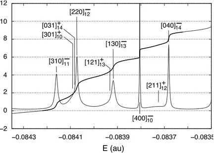
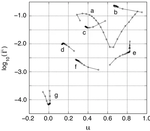
To find the resonance positions it is sufficient to add up the eigenphases from the scattering matrix and fit the result with a linear combination of arcotangent functions plus a smooth polynomial background. This procedure must be applied separately for each isolated group of resonances. Figure 1.6 illustrates the fitting procedure. Total phaseshift, divided by π, around an isolated doubly excited states multiplet in 1Po helium manifold below N=5 threshold is reported as a function
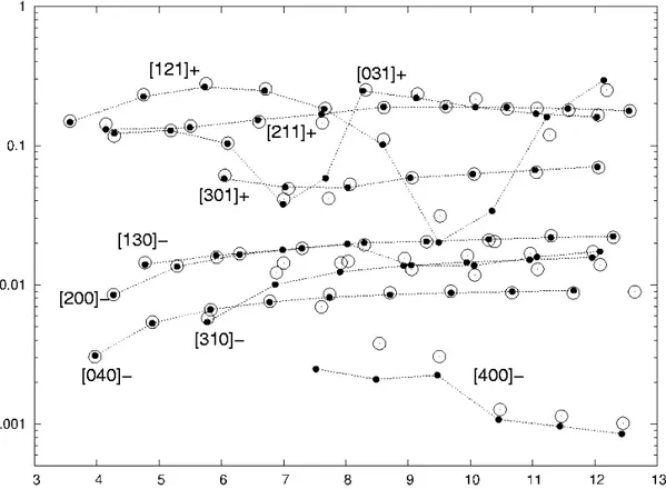
of energy together with its derivative (scaled to fit in the plot), which represents the density of states. The fitting function (nine resonance terms plus a polynomial background of fourth degree) is superposed to the phase shift as a thicker line. The corresponding resonance parameters are reported in table 1.2 (The outer principal quantum number n in the classification of resonances is chosen to match that by Rost et al [99]).
In figure 1.7 a more spectacular example of autoionizing multiplet series is reported: the 3De helium manifold below N=5 threshold.
Huge resonances with widths comparable to or larger than the intermultiplet distance may be missed because they cannot be distinguished from a polynomial background in a small interval. A technique to circumvent this is to subtract progressively the narrower fitted resonances and to repeat the fitting procedure on the residual spectrum.
E (au) [310]11
!
10+ [301] [121]13 [130]13 +!
[400]10!
12 [211]+ 8 6 4 2 0 !2 !0.0843 !0.0841 !0.0839 !0.0837 !0.0835Table 1.2: Parameters of a selected group of 1Po helium resonances below N=5 ionization
threshold, corresponding to the peaks shown in figure 1.6.
[N1N2m]A E (au) Γ/2 (au) [031]+14 -0. 084 080 6.79[-5] -0. 084 092 6.29[-5]a [121]+13 -0. 083 935 4.19[-5] -0. 083 966 5.68[-5]a [211]+12 -0. 083 729 5.76[-5] -0. 083 737 5.97[-5]a [301]+10 -0. 084 087 2.38[-5] -0. 084 103 2.48[-5]a [040]−14 -0. 083 682 2.76[-6] -0. 083 678 2.87[-6]a [130]−13 -0. 083 918 7.79[-6] -0. 083 919 7.60[-6]a [220]−12 -0. 084 073 4.76[-6] -0. 084 079 5.84[-6]a [310]−11 -0. 084 160 6.37[-6] -0. 084 169 5.77[-6]a [400]−10 -0. 083 805 3.77[-7] -0. 083 820 3.21[-7]a a[Rost et al (1997)] [99]
20 18 16 14 12 10 8 6 4 350 300 250 200 150 100 50 0 12 12.6 13.6
Figure 1.7: 3Dehelium total phaseshift divided by π (blue) and state density (red) below N=5
threshold as a function of the effective principal quantum number n∗. In the asymptotic region
each multiplet is formed by twelve resonances, corresponding to the degeneracy of the N=53De
threshold: 5sWd, 5pWp, 5pWf, and 5"W!−2,!,!+2 for " = 2, 3, 4. The excursion of the total
phaseshift in the interval of one effective quantum number reproduces closely this number as the inset shows. The nine narrower resonances are clearly visible as Lorentz peaks in the density of
states, that is the derivative of φtot/π with respect to n∗(The resonances in the inset has actually
been scaled for clarity). As shown in the text, for autoionizing Rydberg resonances the density of states per unit of effective quantum number can be seen as the number of revolutions performed by an electron temporarily captured when scattering off the parent ion.
The derivative of the δsum/π represents the density of states in the continuum
ρ = 1 π
dδ
dE. (1.53)
As first observed by Eisenbud [100], the derivative of the phase shift is proportional to the time delay of an electron scattering off the parent ion
τ = 2!dδ
dE = hρ(E). (1.54)
The first equation in 1.54 is often referred to as the Wigner-Eisenbud relation [101]. For a recent review of time delay in quantum scattering, see De Carvalho et al [102]. In the specific case of photoionization, the long range Coulomb interaction between the parent ion and the leaving photoelectron gives rise to infinitely many metastable states below each ionization threshold, arranged in multiplets. The multiplet series eventually stabilizes in a periodic pattern (that is the derivative of total phaseshift with respect to the effective quantum number n∗ ≡ [2(E
thr − E)]−1/2 converges
2 1
with characteristic sizes rising as n∗2, and periods rising as n∗3, analogously to the
third Kepler’s law. In the case shown in figure 1.7, the impinging electron may perform tens to hundreds revolutions before leaving the ion.
1.8
Radiative K-matrix
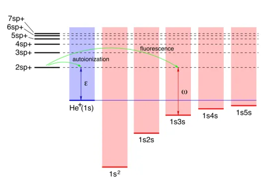
This section is devoted to the treatment of atom and radiation on equal ground. We are not presently interested in high intensity fields but to single photon pro-cesses where the branching ratios of fluorescence channels might be comparable to those of autoionization channels. In this case the ion yield spectrum, what is often actually measured in photoionization experiments, ceases to reproduce the absorp-tion cross secabsorp-tion, while the fluorescence yield spectrum grows complementarily. One expects also to find larger resonances and a qualitative modification of spec-tra: as the incident photon energy approaches a given photoionization threshold, the autoionization width gets narrower while the fluorescence width converges to a finite value and eventually dominates giving rise to a complete superposition of autoionizing states.
This idea has already be exploited by a number of authors. General theoretical formulation of the so called radiation damping can be found in [103–105]. The first application to the radiative decay on an isolated resonance have been pre-sented by Berrington and coworkers in 1990 [106]. In 1995 Robicheaux, Gorczyca, Pindzola and Badnell described in detail the inclusion of radiation damping in the close coupling equations with the “pole approximation”, obtained neglecting the channel-channel interaction through emission and absorption of virtual photons.
In the same way we defined a partial wave channel (see eq. 1.17), we can define a fluorescence channel, coupling to a bound state φa a photon with definite
spherical symmetry j, electric (λ = +) or magnetic (λ =−) character, and energy ω (see appendix B for definitions)
|φΓ ajλE& = ! maµ CLM Lama,jµ φLamaSσ ⊗ b (λ)† ωjµ|−&. (1.56)
As long as the electronic spin is a constant of motion, we can couple the angular momentum of the field to the orbital angular momentum of the electrons. More-over, when the A field is taken as uniform, the A2 term in the hamiltonian can be
%φΓajλω|H|φΓajλω!& = (Ea+ ω) δ(ω− ω") (1.57) 1s2 He (1s)+ 2sp+ 3sp+ 4sp+ 5sp+ 7sp+ 6sp+ 1s5s 1s4s 1s3s 1s2s fluorescence ! " autoionization
Figure 1.8: Schematic representation of autoionization and fluorescence decay channels The close coupling autoionization wave functions are seeked then in the follow-ing form
|Ψ℘αE& = |φαE&+
! γ ! -d)|φγ'& ℘ E− )Kγ';αE+ ! d - Ωd dω|d⊗ω& ℘ E− Ed− ω Kdω;αE (1.58) where in |d ⊗ ω& the bound state d is coupled to a dipole photon to form a state with the same symmetry of autoionization channels|φαE&. The ultraviolet cutoffs
Ωd have been introduced to regularize the integrals and can be chosen in such a
way that they do not appear in the final, considerably simplified equations. A similar expression holds for the fluorescence channels
|Ψ℘aω& = |a⊗ω&+
! γ ! -d)|φγ'& ℘ E− )Kγ';aω+ ! d - Ωd dω"|d⊗ω"& ℘ E− Ed− ω" Kdω!;aω (1.59) where it is understood that E = Ea+ ω. These equations are transformed into a
system of coupled integral equations through passages analogous to those followed in the previous sections. All the details and definitions of symbols are given in appendix E. The final system of equations for the components on autoionization
to the case where the fluorescence channels are completely omitted. This remains thus the only time-consuming step. The components on the fluorescence channels are given in terms of the former solutions by
Kbω,αE = Cω1/2{∇
b,αE+∇b,•P(E)K•,αE} (1.62)
Kbω!,aω = Cω"1/2∇b,•P(E)K•,aω (1.63)
The on-shell K-matrix is manifestly symmetric. Even if the matter K-matrix is left unchanged, the transition matrices T± do change, and so does the scattering
matrix S as well as all the resonance widths.
In the case of just one discrete state i coupled to a fluorescence channel a⊗ ω a simple calculation leads to the following expression for the radiative linewidth:
Γ(E) = 2πC2(E− Ea)|∇a,i|2
which coincides with the well known radiative decay rate of i. In appendix E, this method is applied, as an example, to the radiative decay of an autoionizing state.
Singlet helium photoionization
2.1
Introduction
Despite the apparent simplicity of the helium system, its photoionization spectrum displays a richness of details that has begun to be fully appreciated only in the last two decades. The N-th ion threshold is announced by a resonance multiplet series with (2N − 1) terms which, for small N (N ! 7) [23], can be labelled according to a set of approximate quantum numbers. When in a doubly excited state the outer electron is so far away from the nucleus that its effects on the inner electron can be approximated by a constant electric field, the available configurations of the inner electron are adequately labeled with the Stark quantum numbers N1,
N2 and m [107]. A set of Stark quantum numbers therefore identify an
asymp-totic Rydberg series of doubly excited states with assigned inner electron principal quantum number N = N1 + N2 +|m| + 1, total spin, angular momentum, and
parity. A single term in a series is identified with an additional index n for the principal quantum number of the outer electron: [N1N2m]n. A further symbol
A = +/− /0, originating in the molecular approximation scheme, is generally also specified (for further details on the many almost equivalent classification schemes of doubly excited states, see appendix F).
When many interacting doubly excited states with different N occur in the same energy interval, though, these approximate quantum numbers loose their meaning. This happens already below the N=4 threshold where, in the1Po symmetry, the
first intruder state, [031]+
5, appears. As the energy rises, the increasing number of
intruder states perturb the regularity of the photoionization spectrum [22, 24, 108] until, beyond N=9, it is virtually lost [23–25, 109].
Much theoretical work has been dedicated to the detailed study of anomalies above N = 4 threshold [21–24,99,108,110]. Nevertheless, not earlier than a couple of years ago (2006), the aforementioned very first anomaly in the photoionization spectrum of helium was still only experimentally resolved [21]. This is because the [031]+5 perturber, which falls just∼ 10 meV below the N = 4 threshold, affects the underlying autoionizing Rydberg series in a region where the principal quantum number n of the outer electron is so large, n≥ 14, to seriously challenge ordinary
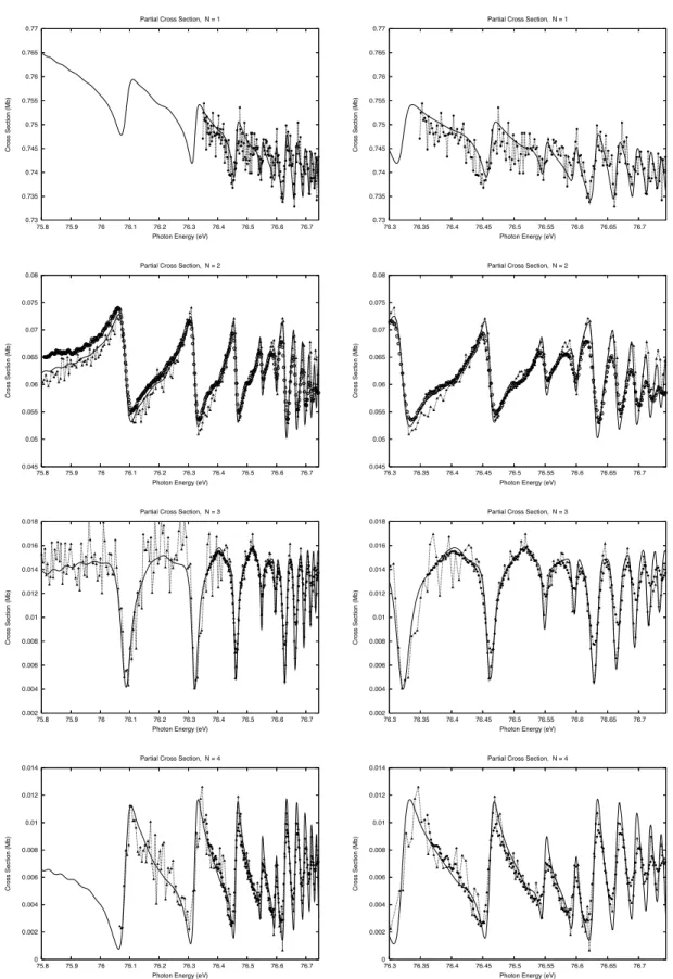
R-tion cross secR-tion (either total or partial) of helium is entirely described by a single dipole anisotropy parameter β. As far as we know, the first and only measurements of the partial cross sections asymmetry parameters βN below N=6 are reported as
preliminary data by Jiang and P¨uttner in Jiang PhD thesis [112]. A theoretical investigation of the photoionization spectrum under N=5 and N=6 thresholds was therefore undertaken [113] in order to reproduce their experimental findings. In sections 2.3 and 2.4 we discuss those results. We find a good agreement with all the available published data and a semi-quantitative agreement with Jiang and P¨uttner’s β6
N’s.
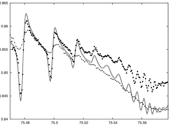
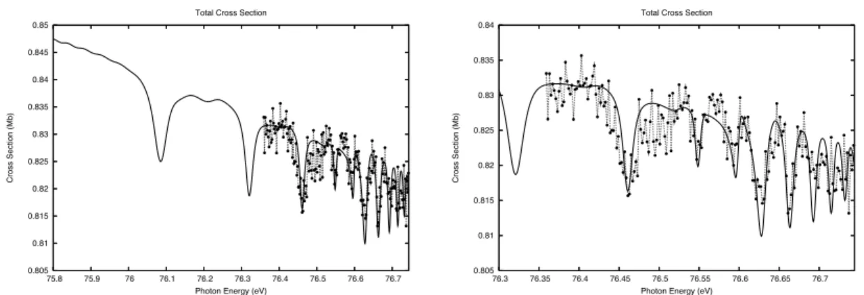
When non dipolar interaction terms between the atom and the incident radia-tion field are taken into account, the many multipolar amplitudes resulting in the same final quantum state give rise to interference effects that alter the photoelec-tron dipolar angular distribution (see appendix B). To measure these effects in helium at low energies is particularly challenging as helium is much smaller than the employed radiation wavelength and they are consequently also small. In prox-imity of resonance features of both dipolar and quadrupolar electric (the leading non dipolar) cross sections, though, the latter may even become dominant, result-ing in a sizable peak in the backward-forward photoelectron anisotropy, provided that the resolution is sufficiently high to resolve those resonances. The first success-ful measurement of this interference effect has been performed in 2002 by Krassig et al [114], but have not been reproduced yet with an ab initio calculation. In section 2.5 a set of such calculations is presented. A good quantitative agreement is found, with the exception of the immediate neighborhood of the dipolar Fano profile minimum, where the simulated nondipole anisotropy parameter is found to depend strongly on the experimental energy resolution.
2.2
[031]
+5, the first intruder state
Let summarize briefly what is expected below the N = 4 threshold. The 1Po
resonances accumulating at threshold are classified in seven series with different parabolic quantum numbers [N1N2m]A [99, 115]:
[021]+, [111]+, [201]+, [030]−, [120]−, [210]−, [300]−.
The nine-fold degenerate underlying continuum where these resonances are embed-ded can be partitioned itself within the parabolic quantum number scheme:
![Figure 2.8: Asymmetry parameters below N=5 threshold compared with data by Menzel et al • · · · •, circ · · · ◦ [125] and Jiang et al " · · · " [110].](https://thumb-eu.123doks.com/thumbv2/123dokorg/4938335.52000/48.918.157.765.256.925/figure-asymmetry-parameters-threshold-compared-data-menzel-jiang.webp)