Spectropolarimetric techniques and applications to stellar magnetism

UNIVERSITA’ DEGLI STUDI DI

CATANIA

DIPARTIMENTO DI FISICA E ASTRONOMIA

DOTTORATO DI RICERCA XXX CICLO

By

C

ESARE

S

CALIA

S

PECTROPOLARIMETRIC TECHNIQUES AND APPLICATIONS TO STELLAR MAGNETISM

A

BSTRACT

T

his dissertation is aimed at the measurement and the characterization of stellar magnetic fields, which are one of the most challenging topics in the modern astrophysics. They are been detected in almost all the stellar evolutionary stages, from pre-main sequence to degenerate stars. They are the keys from the understanding of several phenomena, such as accretion on pre-main sequence stars, stellar activity and spots and they are also important in order to investigate possible false detections of exoplanets and to characterize star-planet interactions. In particular, this thesis focus on the study of upper main sequence, active solar analogs and stars hosting planet, with particular attention on evolved stars.

Stellar magnetic fields can be measured through the polarization and the splitting due to Zeeman effects, from spectropolarimetric observations. In particular, this dissertation employs archive data of Narval and HARPSpol and it is based on observations obtained with the instruments CAOS (Catania Astrophysical Observatory Spectropolarimeter) in more than hundred nights, during the period of the thesis.

Full Stokes observations of the magnetic Ap starβ CrB are used in order to determine the transversal component and the angle of the magnetic fields.

The observations of a sample of 22 stars with detected planets are used in order to study the impact of the presence of the field; results show that the 47% of the giants and the 40% of the main sequence stars in the sample host magnetic fields. In particular, the field strenghts of the giant stars show a correlation with the rotational period, which can be connected to the presence of a dynamo process driven by rotation. Measurements are performed throught the Least Square Deconvolution technique, using a code that was implemented and tested during the period of thesis.

Furthermore, a new technique for the measurement of the effective magnetic field from high-resolution observations is introduced. This technique, called multi-line slope method, is tested with synthetic spectra and it is applied to a dataset of spectropolari-metric observations of the active star² Eri, which spans 9 years from 2007 to 2016. The temporal analysis allows to determine a period of variation (P1= 1099 ± 71 d) consistent

with the variation of the activity index. This measurement represents the first estimation of the period of the cycle of a star obtained from direct measurements of the magnetic field.

A

CKNOWLEDGMENTS

I

would first like to thank my thesis advisor and mentor Prof. Francesco Leone that guided me since the master and made me a scientist. I would also like to thank Prof. Martin Stift and his wife for the encouraging and Prof. Stefano Bagnulo for his support. I thank Dr. Luca Fossati and Dr. Alex Martin for time working together and all people of Armagh Observatory.

I would like to thank Manuele Gangi and all the group of the instrument CAOS for all the nights spent together at the telescope. I thank Salvo Guglielmino and all the people of the Catania Astrophysical Observatory for the support.

I also thank Giuseppe Marino and all the people of Gruppo Astrofili Catanesi (GAC) for introducing me into the fascinating world of astronomy.

Finally, I thank my mother for her endless support, my family, and my friends.

This research is based on observations collected at the European Organisation for Astronomical Research in the Southern Hemisphere under ESO programmes 079.D-0178(A), 084.D-0338(A), 086.D-0240(A). This research has used the PolarBase database.

T

ABLE OF

C

ONTENTS

Page

List of Tables xi

List of Figures xv

1 Introduction 1

1.1 Overview on the stellar magnetic field . . . 1

1.1.1 Pre-main sequence stars . . . 2

1.1.2 Solar magnetic field . . . 4

1.1.3 Late type stars . . . 7

1.1.4 Early type stars . . . 8

1.1.5 White dwarfs . . . 11

1.1.6 Giant stars . . . 12

1.2 Magnetic fields and exoplanets . . . 14

1.3 This work . . . 15

2 Description of polarized light 17 2.1 The polarization Ellipse and Stokes Parameters . . . 17

2.1.1 Properties of the Stokes Parameters . . . 21

2.2 Zeeman effect . . . 22

2.2.1 Analytical expression of Landé factor . . . 23

2.2.2 Transition between two atomic levels . . . 24

2.2.3 Effective Landé factor . . . 26

2.3 Weak field approximation . . . 27

2.3.1 Linear polarisation . . . 28

3 Measurement of polarized light 29 3.1 Polarizers . . . 29

TABLE OF CONTENTS

3.1.1 Polarizing beam splitters . . . 30

3.2 Retarders . . . 33

3.2.1 TIR retarders . . . 35

3.3 Prototype of a polarimeter . . . 37

3.3.1 Linear polarization . . . 39

3.3.2 Circular polarization . . . 40

3.4 Problems on polarization measurements . . . 40

3.4.1 Instrumental sources . . . 40

3.4.2 Atmospheric sources . . . 40

3.5 Instrumental implementation: two beam analyser . . . 41

3.5.1 Four beam procedure . . . 43

3.6 CAOS . . . 43

3.6.1 The polarimeter . . . 45

3.7 CAOS Calibration . . . 46

3.8 Data reduction . . . 48

3.8.1 Calibration . . . 48

3.9 Reduction of the images . . . 49

3.10 Computation of the Stokes parameters . . . 52

4 COSSAM 53 4.1 Radiative transfer for polarized radiation . . . 53

4.2 ADA for astrophysical computation . . . 57

4.3 Numerical solver of Stokes profiles . . . 58

4.4 Cossam extensions . . . 58

5 The trasversal magnetic field ofβCrB 63 5.1 Oblique rotator model . . . 64

5.2 Integrated quantities . . . 66

5.2.1 Effective magnetic field . . . 67

5.2.2 Magnetic field strength . . . 67

5.2.3 Transverse magnetic field . . . 68

5.3 Magnetic field modelling and parametrization . . . 69

5.4 Measurement of the transverse magnetic field . . . 71

5.4.1 Disk integrated relation . . . 73

5.5 HD 137909 . . . 74

TABLE OF CONTENTS

5.7 Modelling magnetic curves . . . 79

5.8 The orientation of the stellar rotational axis . . . 87

6 Magnetic field of stars hosting planet 89 6.1 Least square deconvolution . . . 89

6.2 Effective magnetic field measurement . . . 92

6.3 LSD tests . . . 93

6.4 Target stars . . . 98

6.5 Results . . . 99

6.5.1 Magnetic field strength vs rotational period . . . 101

6.5.2 Questioning of the exoplanet of_{ι Dra . . . 109}

7 The slope method for the measure of the effective magnetic field of cool stars 111 7.1 The slope method . . . 112

7.2 The multi-line slope method . . . 112

7.3 Numerical tests . . . 118

7.4 Noise simulations . . . 120

7.5 Comparison with the Least Square Deconvolution technique . . . 121

7.6 Magnetic field of Epsilon Eridani . . . 122

7.6.1 Questioning about the presence of planets . . . 124

7.6.2 Observations . . . 126

7.6.3 Measurements . . . 126

7.7 Periodicities of effective magnetic field . . . 128

8 Conclusion 135 A Appendix A: COSSAM applications to open clusters 139 A.1 Observations . . . 140

A.2 Abundance Analysis . . . 141

A.2.1 Cossam Simple . . . 141

A.2.2 Determination of stellar parameters . . . 141

A.2.3 Stars selection . . . 142

A.2.4 Abundance measurement . . . 143

A.3 Cluster’s membership . . . 143

A.4 Results and discussion . . . 146

TABLE OF CONTENTS

A.4.2 The blue straggler HD170054 . . . 149 A.4.3 Stellar metallicity . . . 152 A.4.4 HR diagrams . . . 153

L

IST OF

T

ABLES

TABLE Page

3.1 Order by order wavelength coverage. Columns report aperture numbers (A), diffraction orders (O), first and last wavelengths. . . 51

5.1 Ratio between the measured transverse field and the expected value. The equatorial velocity is equal to the projected velocity. . . 74 5.2 Data set of CAOS observation ofβCrB. . . 77 5.3 Measured transverse magnetic field ofβCrB. Eq 5.27 was applied to CAOS

spectra in the range 5000 to 6000 Å and to a single iron line. . . 79 5.4 Effective magnetic field ofβ CrB (Mathys, 1994). . . 82 5.5 Surface field ofβ CrB (Mathys et al., 1997). . . 83 6.1 Results of effective magnetic field measurement from the Least Square

De-convolution profiles obtained by COSSAM simulations for different values of rotational velocity and effective magnetic field. The percentages are computed as the difference between the measured and the syntetic values. . . 96 6.2 Effective magnetic field measures of² Eri observed with CAOS. . . 96 6.3 Table of stars observed with CAOS. The reference are respectively: [1] (Valenti

& Fischer, 2005), [2] (Jofré et al., 2015), [3] (Takeda et al., 2008), [4] (Trifonov et al., 2014), [5] (Soubiran et al., 2016), [6] (Wu et al., 2011), [7] (Mortier et al., 2013), [8] (Sato et al., 2012), [9] (Massarotti et al., 2008), [10] (Zoghbi, 2011), [11] (de Medeiros & Mayor, 1999), [12] (De Medeiros et al., 2002), [13] (Hoffleit & Warren, 1995), [14] (Richichi et al., 2005), [15] (Richichi & Percheron, 2002), [16] (Baines et al., 2008), [17] (Borde et al., 2002), [18] (Bourges et al., 2017), [19] (ESA, 1997), [20] (Simpson et al., 2010) and [21] (Kane et al., 2010). The symbol * is used for indicate values estimated from the interferometric diameter (see text). . . 98

LIST OFTABLES

6.4 Effective magnetic field measurements on the sample of stars observed with

CAOS. . . 99

7.1 Results of effective magnetic field measurements from the multi-line slope method (Bms) and from the slope method and from the slope method applied on all the simulated data points in the spectral region (Bslope) vs rotational velocity. The input effective magnetic field is Binp= -6.45 G. . . 118

7.2 Results of effective magnetic field measurements from the multi-line slope method (Bms) and from the slope method applied on all the simulated data points in the spectral region from 500 nm to 600 nm (Bslope) vs effective magnetic field strength. The rotational velocity is v sin(i) =3 km s−1_{. . . 119}

7.3 Results of the effective magnetic field measurements from the multi-line slope method (Bms) and from the slope method applied on all the simulated data points in a region from 500 nm to 550 nm (Bslope) in the case of a dipole shifted from the centre of the star. . . 119

7.4 Results of effective magnetic field measurements from the multi-line slope method (Bms) vs S/N ratio. The input effective magnetic field is Binp= 6.35 G and v sin(i) = 3 km s−1.σBmsis the standard deviation of the measures in the simulation (details in the text). The spectral region is between 500 nm to 600 nm. . . 119

7.5 Effective magnetic field measures of²Eri. . . 126

7.6 Table of the values of A0. . . 129

A.1 Gratings employed for the FLAMES/GIRAFFE observations. . . 140

A.2 Mean kinematic values of NGC6633. . . 146

A.3 List of programme star of NGC6633. The probability to be member is taken from Sanders (1973). The symbol * in the spectral-type column (Column 3) means that this was estimated from our determined effective temperature according to Currie et al. (2010). The J and K magnitude are taken from 2Mass catalogue (Cutri et al., 2003). The B and V magnitude are taken from APASS catalogue (Henden et al., 2016). The symbol * in the proper motion columns means that the value are taken from Gaia Collaboration (2016), for the UCAC stars the values are taken from UCAC2 catalogue (Zacharias et al., 2004) while for all the other stars are taken from Tycho-2 catalogue (Høg et al., 2000). . . 147

LIST OFTABLES

A.5 Abundance of elements for analysed non member stars, given in log(N/H). In parenthesis the lower and upper limit of the error. The last row gives the solar abundances from Asplund et al. (2009). . . 150 A.6 Abundance of elements for analysed member stars of NGC6633, given in

log(N/H). In parenthesis the lower and upper limit of the error. The last row gives the solar abundances from Asplund et al. (2009). . . 151 A.7 Abundance of elements for analysed member stars of NGC6633, given in

log(N/H). In parenthesis the lower and upper limit of the error. The last row gives the solar abundances from Asplund et al. (2009). . . 152 A.8 log(L /L¯), log(Teff), M/M¯and fractional ageτ for members star of NGC6633.155

L

IST OF

F

IGURES

FIGURE Page

1.1 Magnetic field over the HR diagram (Berdyugina, 2009). Percentage indicates the fraction of stars with magnetic field; stars with convective and radiative

envelopes are respectively at the right and left side of the dashed line. . . 2

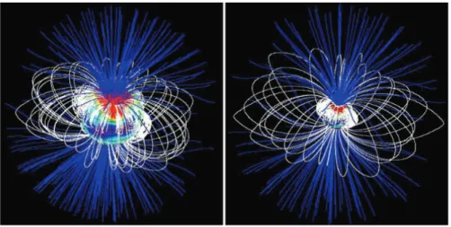
1.2 Topology of the magnetosphere of the T Tauri BP Tau (Donati et al., 2008). . . 3

1.3 Butterfly diagram of sunspots since May 1874. Credits NASA (https:// solarscience.msfc.nasa.gov/SunspotCycle.shtml). . . 4

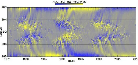
1.4 Synoptic magnetogram of the radial component of the solar surface mag-netic field. Credits NASA (https://solarscience.msfc.nasa.gov/images/ magbfly.jpg). . . 5

1.5 The average quiet-Sun temperature distribution . . . 7

1.6 Magnetic activity for Sun and other stars (Baliunas et al., 1995). . . 9

1.7 Stellar magnetic activity vs rotation (Noyes et al., 1984). . . 10

1.8 Detections of X-rays emission of single stars from ROSAT All-Sky Survey (Haisch et al., 1991). . . 13

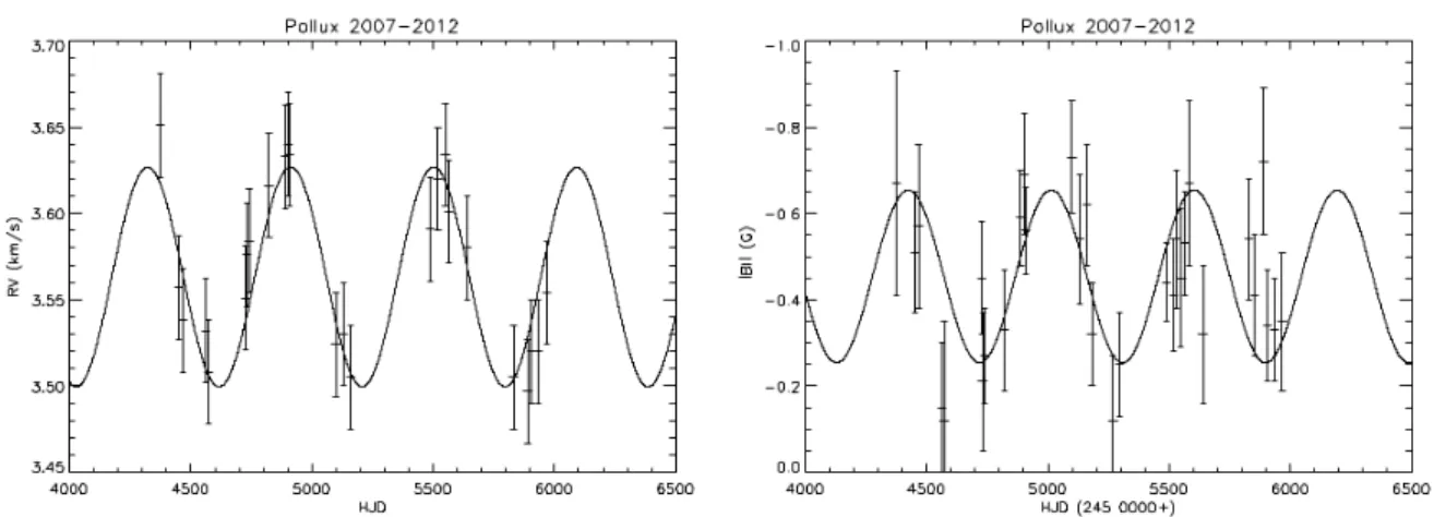
1.9 Radial velocity (left) and magnetic field (right) variations of Pollux, from Aurière et al. (2014). A sinusoidal fit with P = 589.64 d is showed in both figures. 15 2.1 Polarization ellipse (Degl’Innocenti & Landolfi, 2006). . . 18

2.2 Rotation of the reference direction with the angleα (Degl’Innocenti & Landolfi, 2006). . . 21

2.3 Polarization properties of Zeeman effect (Degl’Innocenti & Landolfi, 2006). . . 25

2.4 Examples of Zeeman patterns (Stift & Leone, 2003). . . 26

2.5 Anglesθ and χ of the magnetic field direction Degl’Innocenti & Landolfi (2006). 28 3.1 Rochon prism (Clarke, 2009). . . 31

3.2 Wollaston prism for positive (quartz) or negative (calcite) birefringence (Clarke, 2009). . . 31

LIST OFFIGURES

3.3 Glan-Foucault prism (Clarke, 2009). . . 32

3.4 Foster prism (Clarke, 1965b). . . 32

3.5 Savart plate. a) Two blocks of calcite; b) View of the displacement (Clarke, 2009). . . 33

3.6 General quarter-wave plate (left) and half-wave plate (right). Credits Edmund Optics (https://www.edmundoptics.com/resources/application-notes/ optics/understanding-waveplates/). . . 34

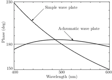
3.7 The phase delay of a compound half-wave plate made of quartz and MgF2, designed to be achromatic at 425 and 575 nm, is compared with a simple plate of quartz cut to be half-wave at 500 nm (Clarke, 2009). . . 35

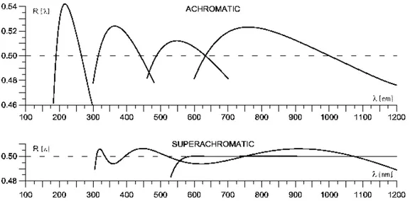
3.8 Comparison between achromatic and superachromatic retarders. Credits Bernard Halle Nachfolger GmbH (http://www.b-halle.de/EN/Catalog/ Retarders/Superachromatic_Quartz_and_MgF2_Retarders.php). . . 36

3.9 Quarter-wave (left) and half-wave (right) Fresnel rhombs (Keller, 2002). . . . 36

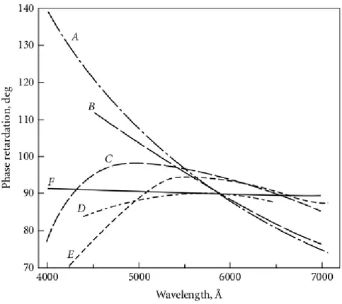
3.10 Phase retardation vs wavelength forλ/4 plates: A, quartz; B, mica; C, stretched plastic film; D, apophyllite; and E, quartz-calcite achromatic combination; F, Fresnel rhomb (Bass et al., 2010). . . 37

3.11 K prism retarder (Moreno, 2004). . . 38

3.12 Prototype of a polarimeter (Landi Degl’Innocenti, 1992). . . 38

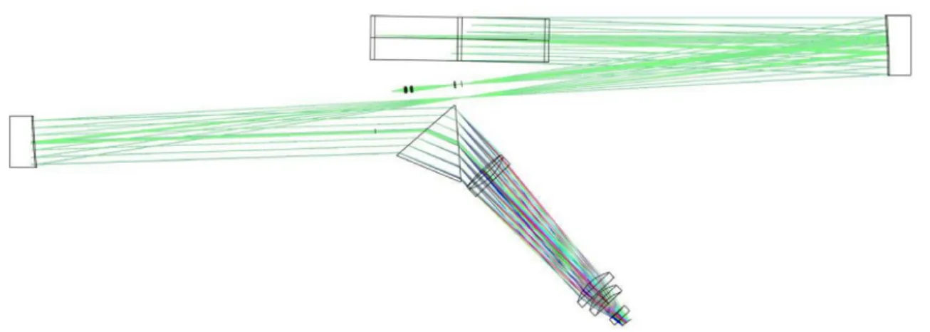
3.13 Optical layout of CAOS as seen from the top (Leone et al., 2016). . . 43

3.14 CAOS camera (Leone et al., 2016). . . 44

3.15 Retardance of CAOS wave plates. . . 46

3.16 Variation of Stokes profiles of Fe II 5018 Å of βCrB. The red curves are obtained with CAOS while the blue are obtained with ESPaDOnS. . . 47

3.17 Top: section of CCD frame showing the 1% scattered light level and its fit-ting with a polynomial function. Bottom: comparison after scattered light subtruction. . . 50

4.1 Polynomial magnetic field configuration with l = 1. . . 60

4.2 Polynomial magnetic field configuration with l = 2. . . 61

4.3 Polynomial magnetic field configuration with l = 3. . . 62

5.1 Magnetic field variations described by the oblique rotator model. Four curves relative to co-latitude of 20◦, 40◦, 60◦and 80◦are shown for each inclination respect to the line of sigh (Stibbs, 1950) . . . 65

LIST OFFIGURES

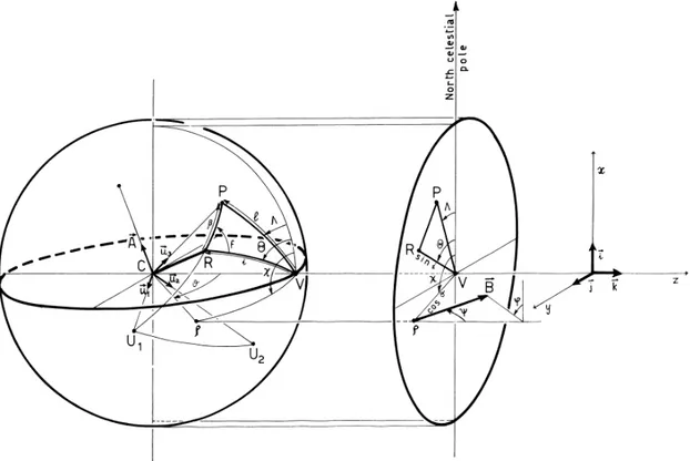
5.2 Geometry of a rotating magnetic star following Landi Degl’Innocenti et al.

(1981). . . 66

5.3 Simulated Stokes parameters (red) for an uniform 1 kG magnetic field, as ob-served at R = 35000 and S/N = 100 (top-left panel), at R = 35000 and S/N = 500 (top-right panel), at R = 115000 and S/N = 100 (bottom-left panel) and R = 115000 and S/N = 500 (bottom-right panel). . . 72

5.4 Measurements of SQfrom COSSAM simulations with B=1 T orthogonal to the rotational axis and along E-W direction, considering a rotational velocity of 3 km s−1(left panel) and 18 km s−1(right panel). . . 73

5.5 Variation of the total surface field |BS| and longitudinal field Beff of β CrB (Preston & Sturch, 1967). . . 75

5.6 Top: Beffmeasures of HD137909 obtained by Wade et al. (2000) (solid circles), Borra & Landstreet (1980) (open squares), Mathys (1991) and Mathys & Hubrig (1997) (open triangles). Bottom: scaled net linear polarization mea-surements obtained from LSD profiles by Wade et al. (2000) and broad-band polarization obtained by Leroy (1995). Credits Wade et al. (2000). . . 76

5.7 Stokes I, V , Q and U of β CrB for the FeII 4923.93 Å (top) and 5018.44 Å (bottom) observed with CAOS. . . 78

5.8 Exemples of measures SQof HD137909. . . 80

5.9 Exemples of measures SUof HD137909. . . 81

5.10 Genetic fit with multipolar magnetic field. . . 84

5.11 Genetic fit with dipolar magnetic field. . . 85

5.12 Examples of configurations with same transverse and longitudinal field but different variations ofχ. Field values are given in units of the polar magnetic field. . . 86

6.1 Comparison between the measurements of the effective magnetic field of² Eri observed with HARPSpol in 2010 (Kochukhov et al., 2011; Olander, 2013). The black points are obtained with our LSD code (black) and red points are the values obtained by Kochukhov et al. (2011). . . 94

6.2 Comparison between the LSD profiles of the magnetic star ² Eri observed with HARPSpol in 2010. On the left, the LSD profiles obtained by Chen & Johns-Krull (2013) (red) and Kochukhov et al. (2011) (black). . . 95

6.3 LSD profiles of the active cool star² Eri observed with CAOS. . . 97

6.4 LSD profiles of giant stars with planet:α Ari (top), 18 Del (center left), ² Tau (center right) and 4 Uma (bottom). . . 102

LIST OFFIGURES

6.5 LSD profiles of giant stars with planet:κ CrB (top), ² CrB (center), Omi Uma (bottom left) andβ Umi (bottom right). . . 103 6.6 LSD profiles of giant stars with planet: 42 Dra (top),γ Cep (center), HD167042

(bottom left) and 11 Com (bottom right). . . 104 6.7 LSD profiles of giant stars with planet: 6 Lyn (top left), HD38529 (top right),

HD210702 (bottom left) and_{ξ Aql (bottom right). . . 105} 6.8 LSD profiles of giant star with planetι Dra. . . 106 6.9 LSD profiles of main sequence stars with planet: 51 Peg (top left), 51 Peg (top

right), HD3651 (center left),υ And (center right) and HD190360 (bottom). . . 107 6.10 LSD profiles of the MIII stars HD6860 (β And). . . 108 6.11 Magnetic field strength vs rotational period. . . 108 6.12 Magnetic field strength vs rotational period in the work of Aurière et al. (2015).109 6.13 Effective magnetic field ofι Dra folded with the rotational period of the planet

ι Dra b Porbital= 510.72 d (Kane et al., 2010). . . 110

7.1 Slope method applied to the magnetic star HD 94660 (top) and to a non magnetic star (bottom) observed with the low resolution instrument FORS1 (Bagnulo et al., 2002). Observations were performed on-axis (at centre of the CCD) and off-axis (at the edges of the CCD) in order to exclude systematics on the measurement. . . 113 7.2 Examples of selected unblended lines (top left), unselected blend lines (top

right) and unselected strong lines (bottom) for a spectra of² Eri observed with HARPSpol on 5thJanuary 2010. . . 115 7.3 Example of normalisation of Stokes I. The red crosses refer to the points used

for the computation of the linear fit, which is reported in blue. . . 116 7.4 Magnetic field measurements of² Eri from HARPSpol data. Top and bottom

panels report respectively Stokes V and the null profiles as a function of the spectral derivative of Stokes I. It is possible to note that the presence of the field is evinced by the slope of the distribution of Stokes V . A flat distribution of the null profile indicates a good quality of the measure. The figure refers, from top to the bottom, to the observation made on the nights of 5, 7 and 9 January 2010. The sizes of the typical error bars are shown in the figures and the S/N is calculated from the standard deviation of the points of the null profile. About 3900 lines are used in the measures. . . 117

LIST OFFIGURES

7.5 Comparison between the multi-line slope method (black) and LSD (red) for

the² Eri HARPSpol observations from the year 2010 (Piskunov et al., 2011;

Kochukhov et al., 2011; Olander, 2013). . . 122 7.6 Comparison between the multi-line slope method (black) and LSD (red) for

the² Eri HARPSpol observations from the year 2010 (Piskunov et al., 2011;

Olander, 2013). . . 123 7.7 Magnetic curves of² Eri folded with the period of rotation of the star Prot= 11.35 d

(Fröhlich, 2007). Cross, diamonds and plus refer to observations obtained res-pectively with NARVAL, HARPSpol and CAOS. Zero phase is equal to MJD 54101 (Jeffers et al., 2014). Magnetic curves are obtained by a fitting through Eq. 7.5 (see text). . . 124 7.8 Wavelet spectrum of S-index measurements from 1968 to 2012 (Metcalfe et al.,

2013). The level of significance is indicated by the color scale; the weakest are white and blue while the strongest are black and red. . . 125 7.9 Top: Cleaned Fourier transform of the effective magnetic field of² Eri (black)

(Deeming, 1975; Roberts et al., 1987) and gaussian fit of the main periods (red). Bottom: Effective magnetic field measures (Table 7.6.3) folded with the two periods. Cross, diamonds and plus refers to observations obtained respectively with NARVAL, HARPSpol and CAOS. . . 130 7.10 S-index measures (Metcalfe et al., 2013) folded with the period P1. . . 131

7.11 Top: Cleaned Fourier transform of A0(black) (Deeming, 1975; Roberts et al.,

1987) and gaussian fit of the main periods (red). Bottom: A0 folded with the

two periods. . . 132 7.12 Temporal variation of A0. . . 133

A.1 A sample of the observed H_β lines. . . 142 A.2 LSD profiles of the possible binary stars. On the top left JEF25, on the top

right TYC445-1684-1, on the center left TYC445-1793-1,on the center right UCAC34148521, on the bottom ClNGC6633VKP129. . . 144 A.3 Color magnitude diagram. Green asterisk are the selected cluster members,

red triangles are the non members, blue cross are binary stars and black triangles are non selected stars. . . 145 A.4 vmicvs Teff. . . 149

LIST OFFIGURES

A.6 Left: spectroscopic HR diagram. Right: HR diagram. The evolutionary track (Bressan et al., 2012) is computed with the age log t = 8.75 (Williams & Bolte, 2007). . . 154

C

H A P T E R

1

I

NTRODUCTION

S

pectropolarimetry is a powerful technique that allows to study several astrophys-ical phenomena, such as circumstellar envelopes, stellar disks, exoplanets and stellar magnetic fields.

Despite the first application of polarimetry in astrophysics was made by Hale (1908) more than a century ago, a great improvement of the knowledge on stellar spectropo-larimetry was possible only in the last few decades, thanks to technological advance and to the introduction of modern spectropolarimeters, which allow to detect the small polarized signals of astrophysical sources.

This work of thesis is devoted to the measure of stellar magnetic fields across the HR diagram. The characteristics of the field changes for different stellar types and they reflect properties of the physical processes which play in stellar atmospheres.

1.1

Overview on the stellar magnetic field

Stellar magnetic fields were detected in almost all the stages of stellar evolution (Fig. 1.1.1), from pre main sequence stars (Johns-Krull, 2007; Hussain & Alecian, 2014) to solar analogue stars (Valenti et al., 1995; Reiners, 2012), upper main sequence stars (Babcock, 1947; Mathys, 2017), giant stars (Konstantinova-Antova et al., 2008; Aurière et al., 2015) and dwarfs (Kemp et al., 1970; Ferrario et al., 2015). A large distinction about the properties of stellar magnetic field can be done according to the presence of a convective envelope at the base of the stellar photosphere. Indeed, stellar convection is

CHAPTER 1. INTRODUCTION

Figure 1.1: Magnetic field over the HR diagram (Berdyugina, 2009). Percentage indicates the fraction of stars with magnetic field; stars with convective and radiative envelopes are respectively at the right and left side of the dashed line.

responsible of phenomena similar to the solar case, such as sunspots, prominences, hot corona and dynamo cycles. Stars without convective envelope possess stable magnetic fields, with large strength values.

1.1.1

Pre-main sequence stars

The study of the magnetic field of pre-main sequence stars is particularly important for stellar evolution, as shown by D’Antona et al. (2000).

Pre main sequence stars are objects in the evolutionary stage of contraction before the zero age main sequence. It is possible to distinguish between:

• T Tauri stars for mass lower than 2M_¯

1.1. OVERVIEW ON THE STELLAR MAGNETIC FIELD

Figure 1.2: Topology of the magnetosphere of the T Tauri BP Tau (Donati et al., 2008).

T Tauri

T Tauri are the progenitors of F, G, K and M stars. They are in the evolutionary stage of the contraction from the Hayashi track, where they are almost fully convective and the energy is released from gravitational collapse.

The magnetic field plays the fundamental role to regulate the accretion of the material on the star. In the magnetic accretion model (Uchida & Shibata, 1984), a strong magnetic field couples disk and star and it is responsible for the loss of star’s angular momentum so that the material can accrete with a rotation rate lower than the breakup velocity. The field is assumed to be dipolar and it stops the disk, forcing the material to accrete through the magnetic field lines (Shu et al., 1994).

Johns-Krull (2007) measured the magnetic field and showed that it reaches values up to a few kG. This strong field is responsible for flares (Guenther & Emerson, 1997) and strong X-ray emissions (Feigelson & Montmerle, 1999).

The geometry of the magnetic field was studied by Johnstone et al. (2014), who related properties of the magnetic field with the phenomenon of convection. They concluded that, when T Tauri are still fully convective, these stars host strong magnetic fields with a simple dipolar structure. This geometry starts to decay and it becomes more complex when the radiative core develops.

Ae / Be Herbig

Ae / Be Herbig stars are progenitors of B and A stars and they were discovered by Herbig (1960). Differently from the case of T Tauri, Herbig stars are expected to have convective

CHAPTER 1. INTRODUCTION

Figure 1.3: Butterfly diagram of sunspots since May 1874. Credits NASA (https:// solarscience.msfc.nasa.gov/SunspotCycle.shtml).

cores surrounded by radiative sub-photospheric envelopes, as showed by Iben (1965). The absence of strong and ordered magnetic field (Wade et al., 2007), suggests that the process of accretion of material in these stars is different from T Tauri. However, models of magnetic field generation and accretion processes are still open questions.

1.1.2

Solar magnetic field

The study of the Sun is important for all stellar and plasma astrophysics because it is the only case where several phenomena, assumed to be present also in other stars, can be seen in detail. Examples are spots, flares and chromospheric and coronal emission processes.

The existence of the solar magnetic field was speculated at the end of XIX century by Bigelow (1891), that observed similarities between the solar corona, during a total eclipse, and the field lines of a magnetized sphere.

The first application of spectropolarimetry in astrophysics, that corresponds to the first discovery of an extraterrestrial magnetic field, was performed by Hale (1908), who measured the magnetic field in sunspots.

Spots on the solar surface are known since 350 BC, from the observations of Theophras-tus (Mestel, 2012). They were observed also by Chinese in 23 BC and they were

rediscov-1.1. OVERVIEW ON THE STELLAR MAGNETIC FIELD

Figure 1.4: Synoptic magnetogram of the radial component of the solar surface magnetic field. Credits NASA (https://solarscience.msfc.nasa.gov/images/magbfly.jpg).

ered by Galileo (Wilson, 2003), who noted also that the period of the rotation of the Sun is close to the lunar month and that spots never appear in the polar regions.

A periodicity of 11 yr in the number of sunspots was first reported by Schwabe (1843). Actually, this value is only an average; the period of the spot’s number is not strictly constant and it varies between 8 and 15 yr (Foukal, 2004). The magnetic nature of the cycle was supposed also by Sabine (1852), that observed the connection between cycle and geomagnetic storms.

The drifts and the positions of spots were studied by Carrington (1859) and Spoerer (1880). They found that spots lie in a region between -30◦_{and +35}◦_{of latitude and they}

appear at lower latitude during the cycle (Spoerer’s law). The plot of the number and the position of the spots, during the cycle, results in the so called butterfly diagram (Maunder, 1913), showed in Fig. 1.1.2.

Hale & Nicholson (1925) studied the polarity of the sunspots and they found that regions of strong magnetic fields are grouped in pairs of opposite polarities and active regions, characterized by opposite polarities, are present in opposite hemispheres (Hale’s law).

Measurements of the integrated magnetic field of the Sun were performed by Babcock & Babcock (1955), that estimated a field value of ' 1 G. Babcock (1959) studied also the variation of the weak large scale magnetic field, observing that it reverses with the same period of the cycle. The variation is between 3 G, during the solar minimum, and 20 G, at the maximum (Priest, 2001). An example of polarity reversal is showed in the synoptic

CHAPTER 1. INTRODUCTION

magnetogram of Fig. 1.1.2 where it is possible to note that change of polarity occurs in the polar regions, at the time of the maximum of the cycle (Charbonneau, 2013).

Observations showed that the visible surface of the Sun, called photosphere, presents a structure at low scale called, called granulation, which is index of the action of stellar convection.

Solar eclipses revealed structures in outer part of the Sun, characterized by an increasing of temperature (Vernazza et al., 1981) and called chromosphere and corona. Because of the temperature distribution, shown in Fig. 1.1.2, different spectral lines can be used in order to obtain information of different regions of the solar atmosphere. In particular, lines like Ca H & H or calcium infrared triplet are important diagnostic indices for the study of the chromospheric active regions (Hale & Ellerman, 1903), which are connected to the magnetic field at the surface.

The cycle of the number of spots impacts all the regions of the solar atmosphere. It produces a cycle in the intensity of the chromospheric emission lines and in the X-ray emission which can increase of factor 100 during the cycle (Priest, 2001).

1.1.2.1 Solar dynamo

The phenomenology of sunspots, resumed for instance by the laws of Hale and Spoorer, indicates the presence of a strong and well organized toroidal magnetic field. Spots are created from the rise of magnetic flux tubes, due to buoyancy effects related to the magnetic activity (Fan, 2009).

Larmor (1919) proposed the idea that an axisymmetric motion of a conductiong fluid, for instance related to solar rotation, could generate and maintain the toroidal field. However, Cowling (1933) showed that a stable axisymmetric magnetic field can not be generated from an axisymmetric current because it incurs the effects of Ohmic dissipation. The problem was solved by Parker (1955), that showed that the break of symmetry, needed in order to avoid the prediction of Cowling’s theorem, could be obtained by the Coriolis twist which raises the material from the convective cells.

Solar dynamo mechanism can be described by the action of two processes:

• differential rotation, which creates the toroidal field from poloidal field, through the shearing of field lines, in a process calledΩeffect (Steenbeck & Krause, 1969). Models suppose that this phenomenon is originated in the region at the base of the convective envelope, called tachocline (Charbonneau, 2010);

1.1. OVERVIEW ON THE STELLAR MAGNETIC FIELD

Figure 1.5: The average quiet-Sun temperature distribution .

• helical turbulence, which twists the rising flux tubes by the Coriolis force. The tubes can reconnect and create the poloidal field from the toroidal, in a process calledα effect.

1.1.3

Late type stars

Late type main sequence stars are objects with surface temperature Ts≤ 104K. Energy in

their core is provided by the p-p chain and they are characterized by a radiative core. This results in a stellar envelope which is convectively unstable because of the high opacity due to ionization of hydrogen and helium. This convective sub photospheric envelope generates a magnetism similar to the solar case. For this reason, stellar magnetic fields

CHAPTER 1. INTRODUCTION

of late type main sequence stars are analyzed extending the results of solar physics. A magnetic field similar to that one of the Sun is very hard to be detected in other stars, because it is characterized by small scale magnetic regions in the stellar surface and their magnetic signals result in a low value, when integrated over the visible stellar hemisphere.

For this reason, indirect indices of magnetism are very important for the study of late type stars. Examples of indicators are the emission chromospheric lines Ca H & K, which can be used in order to detect the presence of magnetic active regions, in analogy of the solar case.

A mile stone on the study of the magnetism of cool stars was the Mt-Wilson survey (Wilson, 1978; Baliunas et al., 1995) which revealed, for the first time, magnetic cycles for stars different from the Sun (Fig. 1.1.3). An other important index of the presence of magnetic field is the X-ray emission which, in analogy to the solar case, is related to the presence of a hot magnetic corona, with temperature close to 106K. X-ray emission of late type stars was measured by Vaiana et al. (1981) and Pallavicini et al. (1981). Schmitt (2001) showed that X-ray emission is present in almost all late type stars, with level also four orders larger than the Sun.

In this context, an important parameter for the magnetism of late type stars is stellar rotation. In particular, magnetic activity showed a correlation with the so called Rossby number Ro= Pobs/τc (Noyes et al., 1984), as showed in Fig. 1.1.3; Ω is the rotational

velocity andτcis the turnover time at the base of the convective envelope.

Magnetic activity for different spectral types was studied by Vaughan & Preston (1980). They found a gap between hot and inactive stars and young, active and fast rotating stars.

1.1.4

Early type stars

Stellar structure of early type stars presents several differences respect to the late type case. These stars are characterized by the presence of a convective core, due to the energy production of the CNO mechanism, and by a radiative stellar envelope.

Following Mestel (2012), the principal properties of the magnetic fields in early type can be resumed in a:

• mean longitudinal component with typical value of few hundred gauss. The largest value for the superficial field is 34kG (Babcock, 1960);

1.1. OVERVIEW ON THE STELLAR MAGNETIC FIELD

CHAPTER 1. INTRODUCTION

Figure 1.7: Stellar magnetic activity vs rotation (Noyes et al., 1984).

• longitudinal and superficial magnetic fields variations with periods of the order of few days. However, in some cases the variation can be of the order of 100 days, several years or decades, such as the case ofγ Equulei which presents a period of the order of a century (P = 97.16 yr) (Bonsack & Pilachowski, 1974; Bychkov et al., 2016);

or decades! Add some references, for instance gamma Equulei

• chemical peculiarity of magnetic stars of types A or B (Ap or Bp);

• variations are due to stellar rotation;

The statistic of the presence of magnetic fields in early type stars presents also differ-ences respect to the lower main sequence case. While almost all late type stars present magnetic activity, only 10% of upper main sequence stars are magnetic. Furthermore, there is an anti-correlation between magnetism and rotational velocity. Indeed, rapidly rotating early type stars are generally non-magnetic.

Variation of magnetic field is described using the oblique rotator model (Stibbs, 1950), where rotational and magnetic axes differ of an angleβ. Observations showed that in

1.1. OVERVIEW ON THE STELLAR MAGNETIC FIELD

a small sample of stars with a period of about one month, β is in the order of 10◦or 20◦(Landstreet & Mathys, 2000).

Magnetic fields of early type stars are stable at long term; this suggests a fossil origin for the magnetic field, which can be created in the molecular cloud where the star formed or in a dynamo process at the time of the pre main sequence phase (Mestel, 2012).

1.1.5

White dwarfs

White dwarfs represent one of the final stages of the stellar evolution (Althaus et al., 2010). They are compact objects, with a temperature in a range between 3000 K to 100000 K and a general slow rotation (≤ 40 km s−1). The majority of white dwarfs (about 80%) is hydrogen rich (H-rich) and the remaining part is helium rich (He-rich). About 25% of H-rich and 20% of He-rich white dwarf are polluted by heavy elements.

Ferrario et al. (2015) showed that the distribution of magnetic fields of white dwarfs seems to be bimodal, one mode characterized by high field strength (from 1 to 1000 MG) and one by low field value (< 0.1 MG).

There are several scenarios proposed in order to explain the magnetic field in white dwarfs, for instance:

• fossil field from the evolution of Ap or Bp stars (Angel et al., 1981; Wickramasinghe & Ferrario, 2005);

• evolution of binary systems through a dynamo that operates in a common envelope phase (Nordhaus et al., 2011) or in a hot corona, created in the merging process of two white dwarfs (García-Berro et al., 2012);

• dynamo mechanism created by the convective mantle of a crystallizing white dwarf (Isern et al., 2017). This is produced in the interior of a white dwarf, composed by a mixture of12C and16O, when the solid oxygen phase crystallizes and settles down, creating a convective mantle of carbon rich liquid by a Rayleigh-Taylor instability (Isern et al., 1997);

• amplification process during the phase of helium burning (Levy & Rose, 1974);

The first two scenarios can explain the magnetism of the group with strong magnetic field while the last can explain the low field group. However, origin of the magnetism in white dwarf is still unknown.

CHAPTER 1. INTRODUCTION

1.1.6

Giant stars

The study of magnetic fields in giant stars is important for stellar evolution theory because it represents the connection stage between white dwarfs and main sequence stars. The field is strictly connected to the evolution of angular momentum and stellar rotation, as stated by Heger et al. (2005), and it could determine the shape of planetary nebulae, as shown by Blackman et al. (2001). Moreover, the field can inhibit the convection processes, which produce the mixing of elements, and it can impact the chemical evolution of the star.

Magnetic fields are expected in the interiors of red giants, from dynamo process related to differential rotation in radiative core (Spruit, 2002), and they are confirmed by the observations of g-mode by asteroseismology (Fuller et al., 2015).

Magnetic fields on the stellar surface are related to the external convective envelope, more than internal dynamo processes (Brandenburg & Subramanian, 2005). Their presence was expected on active giant stars, in order to explain the brightness variation of their spectra by the presence of spots. For instance, Kron (1947) supposed the presence of spots on binary RS Cvn stars AR Lac, composed by a G-K giant and a less massive G-M main sequence star, which was confirmed by the Doppler imaging of the same class star HR 1099 (Vogt & Penrod, 1983); field was also detected in the rapidly rotating FK Com giant stars.

The expected magnetic field of evolved stars has a very complex topology, concentrated in small-scaled structures (Hubrig et al., 1994). For this reason, direct observations of Zeeman effect are difficult, because the average magnetic field results in a very small polarized signal of the order of 10−4.

Direct measures of magnetic fields on the surface of evolved stars started with the detection of the field in V390 Aurigae, obtained by Konstantinova-Antova et al. (2008). The correlation between field and rotation can be used in order to investigate the origin of the magnetic field and, in particular, the possible indication of a dynamo process driven by stellar rotation. This correlation was found for 37 Com (Tsvetkova et al., 2017), V390 Aur (Konstantinova-Antova et al., 2012) and 31 Com (Borisova et al., 2016).

In the other hands, dynamo mechanism can not easily explain the presence of mag-netic field of stars with very long rotational periods. In this case, the magmag-netic field can be assumed to be a fossil remain from previous evolutionary stages, such as a magnetic main sequence star. Landstreet (2004) showed that a kG field, present on the main sequence stars, is expected to decrease to a few G or less in the giant phase, because of the magnetic flux conservation. An example is the case could be EK Eri (Aurière et al.,

1.1. OVERVIEW ON THE STELLAR MAGNETIC FIELD

Figure 1.8: Detections of X-rays emission of single stars from ROSAT All-Sky Survey (Haisch et al., 1991).

2008), which has a rotational period of 300 days and it shows a mostly poloidal magnetic field of 100 G (Aurière et al., 2011). Other examples are 14 Cet (Aurière et al., 2012),

β Cet (Tsvetkova et al., 2013) and OU And (Borisova et al., 2016).

X-ray activity

Indirect evidence of the magnetism of evolved stars was the measure of the X-ray emissions due to confined and very hot plasma in the corona (Vaiana et al., 1981).

Observations show that the X-ray emission stops for stars later than K3, as reported in Fig. 1.8. This phenomenon, called X-ray dividing line (Haisch et al., 1991), is evidence of some change on the dynamo mechanism which drives the magnetic fields in stellar corona.

The idea of a dynamo connected to stellar rotation, as presented by Parker (1955), is confirmed by the correlation between activity and rotation velocity. Pallavicini et al. (1981) found that:

(1.1) LX∼ (v sin(i))2

In order to explain this, Pallavicini et al. (1981) concluded that rotation is an important ingredient that maintains the generated magnetic field.

CHAPTER 1. INTRODUCTION

Dynamo theory is also supported by the observation of the decreasing of X-ray emission over the life time of the star. This result can be explained by a rotational spin down, caused by a mass loss connected to a magnetic stellar wind (Skumanich, 1972).

Relation Eq. 1.1 saturates for fast rotators, how shown by Micela et al. (1985) for a sample of K stars members of the Pleiades cluster. The value of saturation is large for later spectral types and it can be related to bolometric luminosity, as showed by Pizzolato et al. (2003):

(1.2) Psat_rot∼ L−1/2_bol

This result is another indication of the properties of the convective envelope through the spectral types.

1.2

Magnetic fields and exoplanets

Since the first detection of an exoplanet in the star 51 Peg by Mayor & Queloz (1995), the astrophysical community spent a big effort to find and classify as much as possible exoplanets, with the charming desire to find planets similar to the Earth.

Several techniques are applied for this purpose. One of the most important is the radial velocity method, which consists on the measure of variations of the Doppler shift, that is assumed to be related to the gravitational pull due to the presence of a possible orbiting planet. At the moment, 456 extrasolar planets were found with this technique. However, this method can lead to false detections because of the effects of surface magnetic fields. Indeed, analyzing the case of HD 166435, Queloz et al. (2001) showed that the surface magnetic activity of the star can produce a similar signal, in radial velocity, found in stars with true planetary motions. Other false detections were claimed in the years, such as the case of HD 219542 (Desidera et al., 2004), HD 200466 (Carolo et al., 2014) and HD 99492 (Kane et al., 2016). In this context, the direct detection of stellar magnetic field can be used in order to select cases of possible false exoplanets.

The study of the modulation of the magnetic field can be used directly for test the presence of exoplanets. An important case is Pollux, where a planet was found by Hatzes & Cochran (1993) and it was confirmed by Hatzes et al. (2006) but the spectropolarimetric observations of Aurière et al. (2014) revealed that the period of radial velocity and magnetic field are coincident, as shown in Fig. 1.2. Hence, they claimed that spots, associated with the magnetic poles, explain the variation of radial velocity and they make the hypothesis of exoplanet unnecessary.

1.3. THIS WORK

Figure 1.9: Radial velocity (left) and magnetic field (right) variations of Pollux, from Aurière et al. (2014). A sinusoidal fit with P = 589.64 d is showed in both figures.

Magnetic fields are also important in order to study the interaction between stars and planets (Preusse et al., 2006) and the environment around planet-hosting stars (Alvarado-Gómez et al., 2016).

1.3

This work

This work of thesis is devoted to the measurement and the analysis of stellar magnetic fields.

During the work, we described the general techniques for the observation of stellar polarisation and we developed methods of magnetic field diagnostic, in order to study the fields across the HR-diagram, from the main sequence to giant stars.

The aim was to obtain an observational report, in order to characterize the behavior of the magnetic field and to put it in correlation with stellar properties, such as stellar rotation in the case of giant stars, activity index for late type stars or magnetic field geometry in the case of early type magnetic stars.

Furthermore, we showed how the analysis of the temporal variability can be used in order to estimate important stellar parameters. For instance we estimated the radius of the early type stars, the dynamo period of cool stars and we question the detection of one exoplanet.

After a general description of the polarised radiation in Chapt. 2, we introduced the observational techniques used in stellar spettropolarimetry in Chapt. 3, giving partic-ular attention to the description of the instrument Catania Astrophysical Observatory

CHAPTER 1. INTRODUCTION

Spectropolarimeter (CAOS), which was also calibrated during the period of the thesis. Chapt. 4 described the code COSSAM, which was used in order to compute synthetic polarised spectra, representing an important tool for the physical interpretation of the observations. In particular, during the Ph. D. we modified COSSAM in order to include a polynomial expansion for the stellar magnetic field.

The study of the linear polarisation of the early type starβ CrB is reported in Chapt. 5, where we showed how it allows to constrain parameters of the magnetic field geometry and, in this way, it is possible to estimate stellar radius and the orientation of the rotational axis in the sky.

Chapt. 6 is devoted to the analysis of a sample of star hosting planet, with a particular attention to the study of magnetic fields in evolved stars. These measurements were performed through the Least Square Deconvolution using a code that was implemented and tested during the work of thesis.

The analysis of the field in cool main sequence stars is showed in Chapt. 7, where we introduced a new technique, called multi-line slope method, that was used in order to study the temporal variability of the star² Eri. Final conclusions are reported in Chapt 8.

C

H A P T E R

2

D

ESCRIPTION OF POLARIZED LIGHT

T

he astrophysical investigation of the universe is historically performed by means of the electromagnetic waves. However, because technological limitations, in the past it was mainly performed the analysis of the direction (astrometry) and the intensity (spectroscopy) of the light.

This chapter is devoted to the description of a third aspect of the electromagnetic radiation, more difficult to measure, called polarization: the physical quantity associated with the characteristics of the orientation of the electric field vector in time and space.

2.1

The polarization Ellipse and Stokes Parameters

This description and nomenclature of polarization follows Degl’Innocenti & Landolfi (2006).

In classical physics, it is possible to describe, in a simple way, the idealized case of a pure monochromatic plane wave propagating in vacuum; this treatment can be performed equivalently by the use of the electric or the magnetic field vector. Usually, the representation in terms of the electric field is preferred because detectors are generally build using materials whose interaction with the electromagnetic radiation is dominated by the electric vector.

In a right-handed coordinate system, with the z-axis equal to the direction of propa-gation and an x-axis pointing to an arbitrary direction in the plane perpendicular to the

CHAPTER 2. DESCRIPTION OF POLARIZED LIGHT

Figure 2.1: Polarization ellipse (Degl’Innocenti & Landolfi, 2006).

direction of propagation, the electromagnetic wave can be described by:

(2.1) Ex(~r, t) = E1cos(kz − ωt + φ1) = Re[ε1e

i(kz−ωt)_]

E_y(~r, t) = E2cos(kz − ωt + φ2) = Re[ε2ei(kz−ωt)]

with:

(2.2) ε1= E1e

iφ1

ε2= E2eiφ2

where E1, E2,φ1eφ2are four positive constants related to the amplitudes and to the

phases of electric field.

In the most general case, the tip of the electric field vector rotates in time in the x-y plane, describing an ellipse called polarization ellipse (Fig. 2.1).

Calling (x0, y0) the couple of axes obtained by a rotation of (x, y) of an angleα. The electric field in this system is given by:

(2.3) Ex0(t) = (E1C cosφ1+ E2S cosφ2) cos(ωt) + (E1C sinφ1+ E2S sinφ2) sin(ωt) E_y0(t) = (−E₁S cosφ₁+ E₂C cosφ₂) cos(ωt) + (−E₁S sinφ₁+ E₂C sinφ₂) sin(ωt)

where:

(2.4) C = cos α ;S = sin α

The angleα in chosen so that (x0, y0) is coincident with the proper axes of the polar-ization ellipse, with the long axis directed along x0. Calling a the semi-major and b the semi-minor axes, the electric field can be written as:

(2.5) Ex0(t) = a cos(ωt − φ0) E_y0(t) = b cos(ωt − φ₀)

2.1. THE POLARIZATION ELLIPSE AND STOKES PARAMETERS

Comparing Eq. 2.3 and Eq. 2.5, it’s possible to derive:

(2.6)

a cosφ0= E1C cosφ1+ E2S cosφ2

a sinφ0= E1C sinφ1+ E2S sinφ2

b cosφ0= −E1S sinφ1+ E2C sinφ2

b sinφ0= E1S cosφ1− E2C cosφ2

That is equivalent to:

(2.7)

a2_{+ b}2_{= E}2_{1+ E}2₂ ab = −E1E2sin(φ1− φ2)

a2_{− b}2_{= (E}2_{1− E}2₂) cos 2α + 2E1E2cos(φ1− φ2) sin 2α

(E2₁− E2₂) sin 2α = 2E1E2cos(φ1− φ2) cos 2α

The geometrical properties of the polarization ellipse depend on four bilinear com-binations of the electric field components. Introducing the so called Stokes parameters:

(2.8)

I = E2₁+ E2₂ Q = E2₁− E2₂ U = 2E1E2cos(φ1− φ2)

V = 2E1E2sin(φ1− φ2)

the angleα is given by:

(2.9) Q sin 2α = U cos 2α with the constraint:

(2.10) a2− b2= Q cos 2α + U sin 2α

Choosing the interval (0,π) as the interval of definition for α, we obtain for Q 6= 0:

(2.11) α =1 2arctan( U Q) + α0 where: (2.12) _α0=            0 π π/2 i f Q > 0&U > 0 i f Q > 0&U < 0 i f Q < 0

CHAPTER 2. DESCRIPTION OF POLARIZED LIGHT and for Q = 0 (2.13) α =    1 4π 3 4π i f U > 0 i f U < 0

In the case Q = U = 0 the angle α is undefined.

After some algebra, the values of the semi-axis of the polarization ellipse are given by: (2.14) a = 1 2[ p I − V +pI + V ] b =1₂[pI − V −pI + V ]

The four Stokes parameters are not independent, being related by:

(2.15) I2= Q2+ U2+ V2

We can introduce also the ellipticity, that is the ratio of the semi-minor and the semi-major axes of the ellipse. We call the angleβ so that −π₄≤ β ≤ π₄. The sign ofβ is positive in the case of right-handed polarization, while it is negative for the left-handed case.

It can be shown that:

(2.16) tan 2β =_p V

Q2_+U2

Stokes parameters, introduced in Eq. 2.8, can be rewritten as:

(2.17)

I = ε∗₁ε1+ ε∗₂ε2

Q = ε∗₁ε1− ε∗₂ε2

U = ε∗₁ε2+ ε∗₂ε1

V = i(ε∗₁ε2− ε∗₂ε1)

where Eq. 2.2 is used. In this way it is possible to introduce a 2x2 Hermitian matrix, called polarization tensor:

(2.18) Jij= ε∗_iεj= 1 2 Ã I + Q U − iV U + iV I − Q !

The more general case of quasi-monochromatic wave can be obtained through the average over a time much longer than the wave period.

2.1. THE POLARIZATION ELLIPSE AND STOKES PARAMETERS

Figure 2.2: Rotation of the reference direction with the angle_{α (Degl’Innocenti & Landolfi,} 2006).

2.1.1

Properties of the Stokes Parameters

Stokes parameters have important characteristics, which are useful for the next sections. We reported the properties of:

• Rotation of the reference direction:

The Stokes vector in a new system (I0_{, Q}0_{, U}0_{, V}0_{), obtained by a rotation of an angle}

α as shown in Fig. 2.2, can be written as:

(2.19)

I0_{= I}

Q0= cos(2α)Q + sin(2α)U Q0= −sin(2α)Q + cos(2α)U

V0_{= V}

It is possible to note that Stokes I and Stokes V are invariant under rotation, while the linear polarization rotates of an angle 2α in the Q-U plane.

super-CHAPTER 2. DESCRIPTION OF POLARIZED LIGHT

position of an unpolarised beam and a totally polarised beam

(2.20)        I Q U V        =        I −pQ2_+U2_{+ V}2 0 0 0        +        p Q2_+U2_{+ V}2 Q U V       

2.2

Zeeman effect

Polarization arises in the presence of asymmetry in the emitted source or in the medium between the source and the observer. Examples of processes which can produce polariza-tion are:

• reflection

• scattering by grains, molecules and free electrons

• synchrotron emission

• magnetic fields

This work is concentrated on the measure of the stellar magnetic field, whose effects are connected to Zeeman effect. In this case, the preferential direction of the magnetic field breaks the symmetry of the emission, generating circular and linear polarization.

The first explanation of this process was given by Zeeman (1897), who discovered the splitting of the lines and their polarization characteristics in the presence of magnetic fields. Here we reported a quantum description, following Degl’Innocenti & Landolfi (2006).

In the presence of an external and uniform magnetic field, the Hamiltonian of a system of atoms can be described by the addition of an unperturbed Hamiltonian H0and

a magnetic Hamiltonian HB, which is given by:

(2.21) HB= e0h 4πmc(~L + 2~S) ·~B + e2₀ 8mc2(~B ×~r) 2

where~L and~S are the total orbital angular momentum and total spin,~B is the magnetic field vector and~r is the position operator. The second term of Eq. 2.21, called diamagnetic term, is important only for very strong magnetic fields (for instance for white dwarfs) and it can be neglected for purpose of this work.

2.2. ZEEMAN EFFECT

Introducing the Bohr magnetonµ0 the magnetic Hamiltonian can be written:

(2.22) HB= µ0(~L + 2~S) ·~B

If magnetic field is so weak that HB¿ H0 (magnetic energy much smaller than the

energy interval of the unperturbed Hamiltonian), the effects of the magnetic field can be computed using perturbation theory. In this case, called Zeeman regime, the corrections of the unperturbed energy levels E_αJ are given by the diagonalisation of the matrix:

(2.23) ­

αJM|HB| αJM0® = µ0

D

αJM|(~L + 2~S) ·~B|αJM0E= µ0B g MδMM0

where J and M are respectively the total angular momentum and his projection on the z-axis, taken with the direction of the magnetic field, and g is the Landé factor:

(2.24) _{g = 1 +}

D

αJ ||~S||αJE p

J(J+1) (J 6= 0)

The first order eigenvalues of the total Hamiltonian (H0+ HB) are given by:

(2.25) E_αJ+ µ0gBM (M = −J, −J + 1,...,J)

where it is possible to note that the presence of the magnetic field removes the M degeneracy of the unperturbed Hamiltonian. Moreover, the splitting is proportional to the factor g and to the magnetic field.

2.2.1

Analytical expression of Landé factor

Analytical expressions of Landé factor can be found for the cases of coupling between angular momentums.

The easiest situation is the case of L-S coupling. In this scheme, L and S are good quantum number and, through the projection theorem, it is possible to obtain:

(2.26) DβLSJ||~S||βLSJE= D

βLSJM||~S ·~J||βLSJME p

J(J + 1)

whereβ is the generical quantum number of the electronical configuration and: (2.27) ~S ·~J =1 2[J 2 + S2− L2] It is possible to write: (2.28) gLS= 1 + 1 2 J(J + 1) + S(S + 1) − L(L + 1) J(J + 1)

CHAPTER 2. DESCRIPTION OF POLARIZED LIGHT

and, using the compact notation:

(2.29) γ(A,B,C) =A(A + 1) + B(B + 1) − C(C + 1) 2A(A + 1)

Eq. 2.28 can be written as:

(2.30) gLS= 1 + γ(J, S, L)

In the case of j-j coupling scheme, it is possible simplify Eq. 2.24 in a similar way. Considering the levels with orbital angular momentum l1 and l2 and with angular

momentum of spin s1= s2= 1/2, the matrix element can be written as:

(2.31) Dβ(l1s1)j1, (l2s2)j2, J||~S||β(l1s1)j1, (l2s2)j2, J

E

and the Landé factor is given by:

(2.32) gjj= 1 + γ(J, j1, j2)γ(J, 1/2, l1) + γ(J, j2, j1)γ(J, 1/2, l2)

2.2.2

Transition between two atomic levels

In the case of a transition between two atomic levels, with angular momentum J and J0 and Landé factor g and g0, the unperturbed line will split in a collection of components, with frequencies:

(2.33) νJ J_{M M}0 0= ν0+ νL(g0M0− gM)

where the termνLis called Larmor frequency and it is define by:

(2.34) νL=µ0 B h = e0B 4πmc= 1.3996 × 10 6_B

It is possible to write Eq. 2.33 in term of wavelength as:

(2.35) λJ J_{M M}0 0= λ0−∆λB(g0M0− gM)

where the term∆λBis the splitting and it is given by:

(2.36) ∆λB= λ20 νL c = λ2 0e0B 4πmc2 = 4.6686 10 −10_λ2 0B

Among all the possible combinations of M, selection rules have to be considered. They depend on the type of interaction, such as dipole, magnetic-dipole, electric-quadrupole and so on. The simplest cases are the electric-dipole transitions, which are also the most probable to observe. In this case, selection rules are given by:

2.2. ZEEMAN EFFECT

Figure 2.3: Polarization properties of Zeeman effect (Degl’Innocenti & Landolfi, 2006).

The components withδM = −1 are called σrbecause they are shifted to longer

wave-lengths. Their polarisation is generally elliptical and it degenerates into circular, if the components are observed along the direction of the magnetic field, or to linear, if observed along a plane perpendicular to the magnetic field.

The components with δM = +1 are called σb because they are shifted to shorter

wavelengths. The polarization behavior is similar to the case ofσr, an exception is the

sign of the circular polarization which is inverted.

The components withδM = 0 are called π and their polarisation is always parallel to the magnetic field.

Properties of the polarization produced by the Zeeman effects are resumed in Fig. 2.3.

We refered to normal Zeeman effect or normal Zeeman triplet, if the angular mo-mentum of any transition is zero (J = J0= 0) or if the levels have the same Landé factor (g = g0). In this case, only three components are present:σratλ0+ g∆λB,σπatλ0 and

σbatλ0− g∆λB. The other cases are indicated as anomalus Zeeman effect and they can

CHAPTER 2. DESCRIPTION OF POLARIZED LIGHT

Figure 2.4: Examples of Zeeman patterns (Stift & Leone, 2003).

strengths of components can be computed by:

(2.38) J0_{= J + 1 M}0_{= J J}0_{= J − 1} σb M0= M + 1 _{2(J+1)(2J+1)(2J+3)}3(J+M+1)(J+M+2) 3(J−M)(J+M+1)_{2J(J+1)(2J+1)} 3(J−M)(J−M−1)_{2J(2J−1)(2J+1)} π M0_{= M} 3(J−M+1)(J+M+1) 2(J+1)(2J+1)(2J+3) 3M2 J(J+1)(2J+1) J(2J−1)(2J+1)3(J−M)(J+M) σr M0= M − 1 _{2(J+1)(2J+1)(2J+3)}3(J−M+1)(J−M+2) 3(J+M)(J−M+1)_{2J(J+1)(2J+1)} 3(J+M)(J+M−1)_{2J(2J−1)(2J+1)}

2.2.3

Effective Landé factor

The quantity (g0M0− gM) is a property of the particular transition called effective Landé factor. It is related to the sensitivity of the line to the magnetic field and it is defined as the separation of the center of gravity of theσrrespect to the line center, in units of∆λB

2.3. WEAK FIELD APPROXIMATION

Shenstone & Blair (1929) showed that the effective Landé factor geffcan be computed

using: (2.39) geff= 1 2(g1+ g2) + 1 4(g1− g2)d where the term d is given by:

(2.40) d = J1(J1+ 1) − J2(J2+ 1)

Typical values of geffvary from 0.5 to 2.5. Harvey (1973) reported transitions with very

large geff, such as the MnI 4070.278 Å with geff= 3.32, while Sistla & Harvey (1970)

reported lines with geff= 0, such as the FeI 5576.089 Å .

2.3

Weak field approximation

In the cases of weak field, when the Zeeman separation ∆λB of a Zeeman pattern

(assumed as triplet splitting) is small compared to the intrinsic broadening of a spectral line, it is possible to introduce a useful approximation, which is used in order to measure stellar magnetic fields.

In this case, Unno (1956) showed that the circular polarization emerging from a stellar point can be written as:

(2.41) V(λ,θ) =∆λBcosφ

d I(λ,θ) dλ where:

(2.42) ∆λB = 4.67 10−13geffλ2B

andφ and θ are respectively the angle between the magnetic field vector and the line of

sight and the angle between the local surface normal and the line of sight.

Landstreet (1982) showed that the integration over the unresolved stellar disk presents difficulties related to the effects of stellar rotation, which Doppler shift the profiles of different stellar regions, and to the fact that the anglesφ and ∆λB change

over the visible stellar disk.

Assuming that the velocity broadening is small compared to the intrinsic broaden-ing, and neglecting the first effect, Landstreet (1982) showed the relation between the observed Stokes V and the observed Stokes I:

(2.43) V I = −4.67 10 −13_g effλ2Bl d I dλ 1 I

CHAPTER 2. DESCRIPTION OF POLARIZED LIGHT

Figure 2.5: Angles θ and χ of the magnetic field direction Degl’Innocenti & Landolfi (2006).

where Bl is the integral over the visible hemisphere of the magnetic field component

along the line of sight, called effective magnetic field (see Sect. 5.2.1).

2.3.1

Linear polarisation

In the case of weak field approximation (Sect. 2.3), it is possible to obtain equations for linear polarization, similar to Eq. 2.43 for Stokes V (Degl’Innocenti & Landolfi, 2006):

(2.44) Q I = −5.45 10−26G¯λ4B2sin 2_{(θ) cos(2χ)}1 I ∂ 2_I ∂λ2 U I = −5.45 10−26G¯λ 4_B2_sin2_{(θ) sin(2χ)}1 I∂ 2_I ∂λ2

The quantity B2_⊥= B2sin2(θ) is the square root of the transverse component of the magnetic field (see Sect. 5.2.3). The anglesθ and χ are showed in Fig. 2.5.

The term ¯G is called second order effective Landé factor:

(2.45) G = g¯ 2eff− δ with: (2.46) δ = 1 80(g1− g2) 2 (16 s − 7d2− 4) where d is defined in Eq. 2.40 and:

(2.47) s = J1(J1+ 1) + J2(J2+ 1)

g1, g2, J1 and J2 are respectively the Landé factors and the angular momenta of the

levels.

The parameter ¯G plays a similar role to geff for Stokes V . It is possible to note

that ¯G ≤ g2_eff, since δ is equal zero for triplet end non-negative for any Zeeman patter. Moreover, ¯G can assume negative values (about 8% of Fe I have ¯G ≤ 0) and the average value is­_¯

C

H A P T E R

3

M

EASUREMENT OF POLARIZED LIGHT

T

he measurement of Stokes parameters is obtained by means of instruments called polarimeters, which are composed by polarizers and retarders. In this chapter, we illustrated the instrumentation and the techniques used to measure, at high resolution, the polarization of stars; in particular, we concentrated on the description of the spectropolarimeter Catania Astrophysical Observatory Spectropolarimeter (CAOS), which was calibrated and used during the entire period of the Ph. D.

3.1

Polarizers

The polarizer is an optical device which returns a linearly polarized beam, independently of the polarization state of the incident light (Clarke & Grainger, 1971). The direction of the emergent radiation is called transmission axis.

An example of polarizer is the Polaroid, that is characterized by the presence of one single polarized beam at the exit. Mathematically, it can be described by:

(3.1) Ã ²0 a ²0 b ! = eiψ Ã 1 0 0 0 ! Ã ²a ²b ! = eiψ Ã ²a 0 !

where ²a and²b are the components at the entrance of the polariser (along the

trans-mission axis and the orthogonal axis),²0_aand²0_bare the components at the exit of the polariser andψ is a phase difference.

Polarisers can be obtained by means of one or more birefringent crystals, like calcite or quartz. These devices, called polarizing beam splitters, are characterized by the fact