Acknowledgements
I. Regional recessions and recoveries: theories and empirical evidence
I.1 Introduction p. 2 I.2 Resilience and regional evolution p. 3 I.3 Explaining regional evolution p. 8 I.4 The empirics of regional recessions and recoveries p. 20 I.5 Conclusion p. 30 References p. 32
II. Recessions, recoveries and regional resilience: evidence on Italy
II.1Introduction p. 2 II.2 Regional resilience p. 3 II.3 Italian regional evolution: preliminary empirics p. 5 II.4 Econometric analysis p. 9 II.5 Conclusion p. 21 References p. 23 Tables and Figures p. 26 Appendix p. 34
III. An exploratory analysis on the determinants of regional resilience in Italy
III.1 Introduction p. 2 III.2 Theoretical arguments p. 3 III.3 Detecting regional resilience p. 8 III.4 Explaining regional resilience p. 15 III.5 Conclusion p. 25 References p. 27 Tables and Figures p. 30 Appendix p. 41
The motivating research question of the present PhD thesis has been the following: it is not sufficient to choose a question that is interesting and important; you must also choose a question that you have some hope of answering (N.G. Mankiw, 1988). With this in mind, I have tried to shed light on the importance of studying recessions and recoveries at regional level, both in theory and in practice. In particular, the focus has been the development of some econometric tools for analyzing the Italian case. The reader could say if I have been able to provide some answers to this issue.
At least three reasons can sustain this perspective. First, the progressive improvement of data availability at infra national level provides a fertile ground for conducting empirical investigations. Second, the rooted divide showed by different regions within the same country sustains the search for more structured explanations, which can partially rely upon the asymmetric impact of booms and busts. Third, if regions react to fluctuations in a different way, then, modelling place-aware countercyclical monetary and fiscal policies may result more effective.
Three chapters constitute the main structure of this contribution. Chapter I reviews selected theoretical and empirical approaches dealing with regional evolution in order to identify recent developments and extensions incorporating spatial econometrics techniques. Chapter II investigates transient and permanent asymmetric effects of national-wide recessions across Italian regions during the last thirty years, by proposing the recent resilience framework as an helpful synthesis. Chapter III studies the determinants of the uneven cross-regional behaviour during crises and recoveries, by presenting two complementary econometric models, namely a linear vector error correction (VECM) model and a non-linear smooth-transition autoregressive (STAR) specification.
Some of the main results here obtained are: regions within the same country differ in terms of both shock-absorption and post-recession pattern; the broad impact of a common shock shall take into account temporary and persistent effects; differences in recessions and recoveries among areas can be motivated by some elements such as industrial structure, export propensity, human and civic capital, and financial constraints. Moreover, the presence of spatial interdependencies and neighbouring interactions can play a relevant role.
Moving from some of the results here presented, the desirable next step should be addressed towards a deeper analysis of the determinants of regional heterogeneity during recessions and recoveries, cross-country comparisons, the development of a more structured theoretical and empirical background, the assessment of the place-specific impact of countercyclical policies. These and other questions are left for future research.
Acknowledgements (Ringraziamenti)
I ringraziamenti sono per volontà in Italiano, poiché credo così facendo si possa esprimere la mia gratitudine nel modo migliore. Una tesi di dottorato è per natura il completamento di un percorso di studio avanzato al quale hanno contribuito in vario modo diverse persone con le quali ho intrattenuto rapporti professionali e personali durante questi anni.
Innanzitutto, due persone meritano una menzione a parte. Il mio supervisore, prof.ssa Tiziana Cuccia, che mi ha seguito passo dopo passo, introducendomi alla carriera accademica con maestria, correggendomi con sincerità e attenzione, sostenendomi con costanza e spirito propositivo. Il prof. Peter Burridge dell’Univerisità di York, il cui apporto in questa tesi così come in altri lavori è stato fondamentale in termini di rigorosità metodologica, di sviluppo delle principali conclusioni e per il continuo sostegno.
Ci tengo a ringraziare Roberto Cellini per la sua onnipresente disponibilità, i preziosi suggerimenti e le interessanti discussioni. Un grazie particolare va a Paolo Cosseddu, Dario Nicolella, Giuseppe Nicotra, Belmiro Jorge Oliveira per il sincero supporto e le proficue chiacchierate. A vario titolo ringrazio anche: Alberto Abadie (Harvard Kennedy School), Carlo Bianchi (Università di Pisa), Ray Chetty (Harvard University), Maurizio Ferrera (Università di Milano), Bernard Fingleton (University of Cambridge), Paolo Graziano (Università Bocconi), John D. Hey (University of York), Marco Magnani (Harvard Kennedy School), Gian Cesare Romagnoli (Università di Roma Tre), Paul Schweinzer (University of York), Dan Shoag (Harvard Kennedy School), Lanfranco Senn (Università Bocconi), Rodrigo Wagner (Tufts University).
Ci tengo a ringraziare anche Isidoro Mazza, il coordinatore del Dottorato, per la sua disponibilità, correttezza e per l’indispensabile supporto. Come di consueto, sono l’unico responsabile di eventuali errori od omissioni.
theories and empirical evidence
Abstract
The present work represents a survey in regional economics. Specifically, the main objective is a review of the literature and the design of the state of the art of the knowledge about regional recessions and recoveries. The regional resilience framework recently conceptualized offers a helpful starting point for broadening the research perspective on this topic. Selected theoretical and empirical approaches are presented in order to identify transient and permanent effects of national-wide recessions across regions. More recent developments are discussed together with possible future areas of research. Spatial econometrics extensions of empirical models are also presented for dealing with cross-sectional heterogeneity.
Keywords: regional business cycles, disaggregate fluctuations, hysteresis, asymmetric co-movement, dynamic-factor models, SpSVAR, non-linear models.
2
I.Introduction
At least three reasons can motivate the renewed interest for regional topics. First, the presence of long-standing regularities like divergent patterns of convergence across territories and the rooted divide showed by different regions within the same country sustains the search for more structured explanations. Second, in the last two decades data availability at infra national level has substantially improved with detailed micro data now accessible more easily. Third, specific analytical tools such as spatial econometrics and techniques for dealing with cross-sectional heterogeneity have been progressively incorporated in empirical works favouring a deeper knowledge of geographical interdependencies.
In particular, the recent re-discovery of the concept of resilience among regional scientists (see, among others, the special issue of the Cambridge Journal of Regions, Economy and Society, 2010; Martin, 2012) has the value of revitalizing the study of regional recessions and recoveries both in theory and in practice. Although it does not represent a watershed in the existing literature, the resilience framework offers a new perspective for explaining the uneven geography of crises and the asymmetric behaviour of upturns. Not so surprisingly, then, an increasing number of contributions explicitly focus on this issue (Fingleton et al., 2012; Fingleton and Palombi, 2013). Moreover, a larger amount of policymakers both in the US and in Europe is introducing resilience in the policy debate.
This survey aims to shed light on the more recent theoretical and empirical developments concerning the regional evolution of booms and busts. In the next pages, I will try to answer the following questions, recognizing the role of the resilience approach as a useful starting point. How can we identify the impact of economic shocks at infra national level? What are the determinants behind potential territorial differences during crises and recoveries? Can growth differentials across places be explained by dissimilar reactions to shocks? Do national countercyclical policies, monetary and fiscal, require to be integrated by region-specific elements to be more effective?
The remaining of the study is organized as follows. Section II briefly describes the distinctive features of the regional resilience framework and why it can provide an helpful starting point for bridging the gap between alternative traditions in the analysis of regional evolutions. The state of the art of theoretical contributions analysing regional shocks is surveyed in section III. Section IV deals with recent developments in the empirical
3
literature. The final section offers some concluding remarks and possible avenues for future research.
II. Resilience and regional evolution
Resilience is a concept traditionally used in Ecology, Engineering and Physics for analysing the adaptability of particular ecosystems to given disturbances, denoting the resistance of a material or investigating some physical properties in presence of extraordinary events. In Economics, it will probably become soon a buzzword in the sense expressed by Robert Solow for commenting social capital: a new word for reshaping old ideas. Nevertheless, it can contribute to study recessions and recoveries at infra national level in a more integrated perspective, by bringing together two traditional and alternative strands of the literature dealing with the effects of economic shocks.
More specifically, two meanings of resilience have been recently proposed. Engineering resilience denoting the ‘ability of a system to return to, or resume, its assumed stable equilibrium state or configuration following a shock or disturbance’, and ecological resilience defining ‘the scale of shock or disturbance a system can absorb before it is destabilized and moved to another stable state or configuration’ (Martin, 2012). Both concepts share two common features: the presence of a shock hitting a particular (economic) system and the focus on the impact of the generic shock without précising the nature of the shock itself. Moreover, both concepts have been explicitly introduced for studying and comparing regional economic evolutions1.
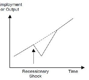
Engineering and ecological resilience, however, considerably differ in terms of both underlying paradigms and consequences arising from the shocks. Indeed, engineering resilience is based upon an implicit equilibrium dynamic where disturbances become relevant only for detecting temporary effects and identifying asymmetries between the bust-phase and the boom-bust-phase across geographical units. Figure 1 illustrates this pattern.
1 In addition, Martin (2012) suggests to integrate the twofold meaning of resilience with four common and related elements: i) the sensitivity of a regional economy to disturbances and disruptions (resistance); ii) the speed and extent of the recovery-phase (recovery); iii) the extent to which the regional economy re-defines its structure (re-orientation); iv) the degree of resumption of the growth path that characterised the regional economy prior to the shock (renewal).
4
Figure 1: Engineering Resilience
Source: Martin, 2012.
As a consequence, a particular fluctuation is able to impose a reduction in the pattern of a variable for a certain period, but its structural behaviour is re-established in the long run (bounce back or peak-reversion effect). In other words, a given economic system, such as a region, fluctuates around its normal level of growth. Disturbances are unpredicted accidents along this trajectory. According to this approach, the decline in GDP and employment does not influence an economy in a perpetual way. A place, such as a region or a city, then, is involved in a self-equilibrating continuous process.
Engineering resilience can be related to traditional business cycles models interested in assessing the transient impact of recessions and the characterizing elements of recoveries. As recently pointed out by Fatás and Mihov (2013), this way of analyzing business cycles dates back at least to Mitchell (1927) and Burns and Mitchell (1946), and it finds an evident application in the ‘plucking’ model of Milton Friedman (1964) and its extensions (Kim and Nelson, 1999)2. In this framework, recessions are extraordinary events
which determines cycles, and there is a relation between a given recessionary event and its recovery. Moreover, the shock-absorption phase can be different (asymmetric) in the post-recessionary period.
Therefore, if we consider engineering resilience at regional level three aspects assume relevance. First, we need to correctly identify each disturbance (i.e. recession) and recovery in terms of both its timing and impact. In general, this means specifying a
2 It is worth noting that Fatás and Mihov (2013) distinguish this approach, which is the basis for the NBER business cycle dating committee methodology, from the so-called trend-cycle approach (Lucas, 1975, 1977; Kydland and Prescott, 1982) where the fluctuations are symmetric and caused by small and frequent shocks affecting a long-run trend.
5
national-wide cycle on the basis of pre-defined criteria: endogenous like the adoption of Markov-switching dating methods or exogenous on the basis of the analysis of peaks and troughs (Hardin and Pagan, 2002).
Second, it can be interesting to evaluate the overall effect of a given cycle by estimating its costs as cumulative losses in employment or GDP experienced during the cycle itself. And, variations in costs among areas within the same nation, captured by special-purpose indexes, can be associated to divergent resilient paths.
Third, it may result helpful to compare the effects of different cycles across time and space in order to provide a deeper knowledge of the geography of crises within a country. For example, regional differences in the timing of a recession (i.e. ‘entry’ and ‘exit’), as documented by Owyang et al. (2005) for the US, can be conceived as a signal of engineering resilience. Regions affected longer than the national average, with anticipated entry and postponed exit, may be candidates to be less (engineering) resilient than the rest of the nation.
At the other end of the spectrum, ecological resilience relies upon the disequilibrium perspective firstly conceptualized by Nicholas Kaldor and Gunnar Myrdal along Keynesian lines. A particular system may develop along not-equilibrating trajectories depending on the initial conditions, history of shocks and agents’ expectations. The presence of a long-run equilibrium, then, is neither assumed nor needed for describing a specific growth path. In this context, recessionary events act as substantive economic disturbances which are able to influence the future development of a given place. Hence, the adverse effects of a crisis become permanent not dying out over the periods and the memory of recessions matters for the future.
This definition of resilience is close to the rooted concept of hysteretic behaviour in Economics. Hysteresis, familiar among Economists since the past, can be defined as a ‘situation where one-time disturbances permanently affect the path of the economy’ (Romer, 2001). As a consequence, a peculiar economic system is not necessarily involved in self-adjusting dynamics, but it can experience multiple patterns in terms of post-recessionary evolution. In other words, the relation between long-run growth and shock-persistence becomes crucial. The four diagrams in figure 2 illustrate different possible post-recessionary patterns for an economy.
6
Figure 2: Ecological Resilience
(A) (B)
(C) (D)
Source: Martin, 2012.
A shock can shift downward the long-run potential of a system while maintaining a constant rate of growth (A). Or, the recessionary event may cause both a decline in the long-run growth and in its variation over time perpetuating a perverse cumulative process (B). Whereas the first case is typical of a territory experiencing a downsize in its structural evolution, the second represents a more negative situation in which a place will suffer prolonged adverse conditions.
Conversely, recovering after a recessionary shock can move the economy over its initial equilibrium with a constant rate after a certain period (C). Or, a given slump could stimulate positive reactions of a system addressing a long-term favourable cumulative
7
process (D). Both situations can be described as processes of creative destruction à la Schumpeter, where the turning point is represented by the adverse shock.
The central element in this case is the relation between a given shock and the induced behaviour of the system under observation. In this sense, we are interested in defining the threshold of shock-absorption required to move from one equilibrium to another: this depends on both the magnitude of the shock and the specific vulnerability of the area3. And, it may also result important to highlight either which kind of equilibrium is
achieved after a shock or what is the out-of-equilibrium pattern followed. Therefore, ecological resilience can be related to models characterized by multiple equilibria and non-linearity.
The concept of resilience, as it has been recently introduced in Economics, offers a worthwhile and quite intuitive stimulus to think hard when dealing with the impact of recessions across areas. On the one side, it combines both the temporary impact of disturbances on a given equilibrium level and the persistent out-of-equilibrium evolutions. On the other side, it provides further motivations for analysing the effects of shocks on economic growth following a place-specific approach (Cerra and Saxena, 2008; Cerra et al., 2013).
Moreover, the intrinsic spatial nature of regional resilience sustains its role of additional informative element for assessing the real impact of monetary policy decisions. Indeed, in presence of regional heterogeneity, it becomes crucial to identify what are the reasons behind monetary policy effectiveness. In particular, a regional-based perspective analysing the three traditional channels associated to monetary policy, namely money, credit and bank lending, is able to look at the transmission of shocks in a more accurate way.4
And, the analysis of the geographical unevenness during recessions and recoveries can act as a helpful starting point for proposing place-based countercyclical policies.
At this point, it is interesting to note how the resilience framework can result helpful for complementing the new directions pursued by the third generation of real business cycles models (Farmer, 2013; Plotnikov, 2013), which are aimed to introduce
3 To be more precise, the specific nature of each shock plays an additional important role. To give an example, as demonstrated by Calvo and Reihnart (2002), currency crises are very different from banking crises if we consider both their origins and effects. While the former have direct implications for trade and public finances, the latter mainly influence credit availability and agents’ expectations in financial markets.
4 Traditionally, three channels of transmission of monetary policy have been identified. The money channel is the relation between a monetary shock and the variation of aggregate demand. The credit channel is the impact of monetary decisions on the broad credit market in terms of loans’ availability lato sensu. The bank lending channel (or narrow credit channel) measures the impact of monetary policy on small banks and small and medium enterprises. For a more detailed discussion, see Owyang and Wall (2005).
8
multiple equilibria in unemployment5. These models rely upon assumptions peculiar to
‘Old Keynesian Economics’ (Farmer, 2008), where the natural rate hypothesis does not hold and deviations of the unemployment rate from its optimal value may be permanent. More on these models will be presented in the next section.
Asking what definition of resilience, engineering or ecological, is able to better describe the pattern of a given economy ex post with respect to a recessionary event is a sort of conundrum. Engineering resilience is probably more appropriated when we adopt a long-term equilibrium perspective and our data do not show particular breaks, while in presence of non-linear evolutions and if we recognize the possibility of modelling out-of-equilibrium economic relations, ecological resilience can result more suitable to analyse the phenomenon at hand.
In accordance with the unified approach heretofore discussed, the next section deals with the current state of the theory of regional recessions and recoveries, by considering both the mainstream equilibrium approach and some disequilibrium-based views.
III. Explaining regional evolution
Before proceeding to outline some of the main contributions dealing with regional recessions and recoveries three premises need to be discussed. First, the starting point of our analysis is a macroeconomic perspective and, therefore, we are interested in modelling the dynamic of aggregate variables leaving only a marginal role to the wide area of study developed by urban studies, economic geography and related disciplines6. Second, in the
following pages we provide a selective review for the purposes of framing the analysis of resilience, recognizing that a synthesis of the theoretical contributions on regional evolution is both cumbersome and outside the boundaries of the present work. Third, the focus on the regional dimension is motivated by the need of understanding the asymmetric behaviour showed by regional fluctuations and the evidence of place-specific elements denoting business cycles (Owyang et al., 2005; Wall, 2012).
5 The expression ‘third generation’ has been applied by Roger Farmer in its recent survey on endogenous real business cycles for distinguishing real business cycles models where multiple equilibria of unemployment are explicitly introduced from the ‘second generation’ (Benhabib and Farmer, 1994) in which there are multiple patterns of adjustment for reaching the same equilibrium level. The first generation refers to the pioneering contributions of Lucas (1977) and Kydland and Prescott (1982).
6 It shall be noted, however, that some aspects hereafter discussed such as labor mobility and spatial interactions are common to both the approach here adopted and other disciplines. This point will be further clarified when explicitly addressed in the main text.
9
A simple Real Business Cycle (RBC) model is firstly introduced and discussed, highlighting its basic characteristics for dealing with economic shocks. More recent developments and some extensions for incorporating regional heterogeneity are also examined. Subsequently, a flexible framework for separating aggregate and regional fluctuations (Quah, 1996) is sketched providing some intuition for its empirical application and possible avenues for future research. Finally, regional hysteresis is presented within a recent RBC framework (Plotnikov, 2013), in combination with its possible causes and consequences.
III.1 (Real) Business Cycle models
Modern Real Business Cycle (RBC) models rely upon the dynamic stochastic general equilibrium approach firstly pioneered by Lucas (1975), Kydland and Prescott (1982) and King, Plosser and Rebelo (1988). Although they represent nowadays the mainstream theoretical view for analysing the economic behaviour of an aggregate economy, it shall be noted that they differ from the data-driven business cycle tradition historically referred to the NBER methodology (Fatás and Mihov, 2013). In particular, the latter is focused on the characterization of aggregate economic series by detecting expansions and contractions without assuming a priori that cycles are deviations from a given equilibrium level (i.e. overcoming the trend-cycle pattern). As a result, the discussion of (traditional) data-driven business cycle models is postponed to the empirical section.
The basic assumptions of a generic RBC model are the following: i) a representative-agent framework; ii) households and firms maximize their objective functions subject to given constraints; iii) the cycle-phase is determined by supply-driven Total Factor Productivity (TFP) shocks or neutral technology shocks (Justiniano et al., 2010); iv) the natural rate hypothesis holds for unemployment; v) agents have rational expectations and markets clear. For a more detailed discussion, see Stadler (1994) and Farmer (2012).
As an example7, let’s consider a representative individual living for an infinite time
period and having preferences described by the relation:
7 The following set up is based upon the basic RBC model presented in King et al. (1988) and recently used by Roger Farmer (2013). Additional specifications will complicate the notation without modifying the basic insights we want to point out.
10
∑
where , , denote the discount factor, consumption and leisure, respectively. Firms produce according to the neoclassical production function
where output ( ) results, as usual, from the combination of capital ( ), labour ( ) and total factor productivity ( ). The law of motion of capital accumlation is
with denoting the depreciation rate of capital and the gross investment. Every period two resource constraints are faced by the representative agent:
where the first relation relates total output to the sum of consumption and investment, and the second one constraints the allocation of time between labour and leisure to the total endowment of time here normalized to 1. Additional constraints are: , ,
, .
Assuming that individual preferences are represented by a logarithmic utility function and production is expressed in the usual Cobb-Douglas form8, the following
system of equations allows to determine the time paths of output, consumption, capital, labour supply and total factor productivity9:
8 More specifically, the two restrictions on preferences must be: a) the intertemporal elasticity of substitution in consumption shall be invariant to the scale of consumption; b) the income and substitution effects linked to labour productivity growth must not interfere with labour supply. Apart from the logarithmic function, the other possible preferences form is the CES representation (King et al,.1988).
9 In addition to equations (1.1)-(1.5), the following boundary conditions must hold: i) ̅̅̅; ii) ̅̅̅; iii) {( ) } , which are the initial condition for capital, the initial condition for TFP and the trasversality condition, respectively.
11 (1.1) (1.2) { ( )} (1.3) (1.4) (1.5)
Equations (1.1) – (1.5) respectively identify: the production function, the capital accumulation relation, the agents’ Euler equation, the first order condition for labour markets, and the evolution of total factor productivity. At this point, it is worth noting that total factor productivity follows a first order autoregressive process where the innovation has distribution . Moreover, in this context five parameters need to be specified, namely the rate of time preference ( ), the elasticity of capital ( ), the labour supply parameter ( ), the autocorrelation coefficient ( ) and the standard deviation ( ) of the disturbance affecting Total Factor Productivity in equation (1.5).
In general, two main categories of disturbances are associated to the basic RBC model10. On the one hand, when consumption smoothing varies over time or unexpected
changes in demand are faced by firms through inventories (Stadler, 1994), an adjustment occurs to re-balancing the evolution of a given economy. On the other hand, random fluctuations of the rate of technological change are able to hit the system under observation. However, only the second mechanism is defined as recession. More importantly, the evolution of an economy is characterized by the continuous presence of fluctuations triggered by the innovation process of TFP, which represent business cycle phases per se. In this context, each shock represents a transitory fluctuations in economic activity away from a permanent level (Morley and Piger, 2012). And, the link between recessions and recoveries is generally missed when applying RBC models.
10 In reality, an additional source of innovation has been found to be relevant in these models: sunspots (Aziaridis, 1981). Sunspots shocks are typically referred to disturbances arising from agent’s beliefs rather than fundamentals.
12
These basic intuitions still remain valid when additional features are introduced to the simple framework previously discussed. In particular, more recent Dynamic Stochastic General Equilibrium (DSGE) models deal with imperfect competition (Rotemberg and Woodford, 1995), taxes (Raurich et al., 2006) and other sources of frictions (Smets and Wouters, 2007) such as labour market rigidities modeled in the spirit of the well-known matching models. In a complementary way, multiple steady-state equilibria have been also explored (Behnabib and Farmer, 1994) within the RBC framework, mostly driven by other forces (e.g. increasing returns-to-scale) than TFP shocks.
Three final comments can be pointed out. First, the underlying behavior of RBC models can be extended in principle to every economic system (i.e. region, city, etc.) without introducing ad hoc specifications. And, this has been the starting point of most of empirical analyses studying RBC at infra national level. In this case, the presence of cross-sectional dependence across places within the same country or the occurrence of spatial interactions are solved by modifying some empirical aspects (e.g. introducing heterogeneity in the error terms or filtering the series for each region). Second, as highlighted by Larry Summers (1986) some years ago, studying the business cycle by means of DSGE models does not necessarily implies providing a better understanding of the evolution of a given economy. This is particularly true when the parameterization shows some arbitrary components (Stiglitz, 2011). As we will see in the next section, the data-driven approach has maintained its explanatory power, though it does not rely upon sophisticated theoretical assumptions. Finally, RBC models do not allow to separate aggregate (i.e. national-wide) from disaggregate (i.e. place-specific) disturbances, limiting the possibility of jointly examining these two sources of business cycle dynamics.
III.2. Aggregate vs disaggregate fluctuations
The contemporaneous identification of aggregate shocks and disaggregate fluctuations is not a trouble-free task from a theoretical point of view, though it has been deliberately assumed as an objective by many empirical contributions (Carlino and Mills, 1998; Clark, 1998; Hamilton and Owyang, 2012). In general, disaggregate elements are considered as a byproduct of aggregate cycles of which they represent a natural complement. To give an idea of the importance of distinguishing aggregate from disaggregate cycles, in this sub-section the simple prototype model firstly presented by Danny Quah (1996) is discussed as its possible extensions.
13
Let’s start by assuming that physical geography is defined as a probability space ( ) with denoting a set of generic (finite or infinite) dimensions (e.g. a circle, a plane, etc.), a relevant subset of , and a probability measure which maps → [0,1]. The function attributes specific characteristics to a given location , and it can be thought as the relation between a particular place (i.e. region or city) and its idiosyncratic features. In this sense, is able to capture both time-invariant and time-varying regional elements.
Considering only labour input , regional output in a representative location is given by the standard technology:
, (1.6)
where, as usual, and decreasing in denotes the productivity of labour.
Combining the relation (1.6) with the measure on locations, we can obtain a probability relation for region-specific characteristics , employment and output . The aggregate total output is obtained by summing up region-specific output for all locations:
̅ ∫ ∫ ( ) (1.7)
and, consequently, the distribution of wages across regions can be easily obtained from:
( ) ( ) (1.8)
When labour is freely mobile across regions, in equilibrium, wages are equal whatever location we consider, and local labour markets clear. More formally,
̅ ( ) (1.9)
14
where ̅ is the common wage at aggregate level. Quah (1996) demonstrates that the following maximization problem
∫ ( )
∫ (1.11)
is solved by a particular employment level belonging to the set of non-negative measureable functions .
For our purposes and without loss of generality11, it can be assumed that the
representative production function has the form , with a scalar, and . Therefore, the marginal productivity of labor is , and local labor demand is ⁄ ⁄ ⁄ As a result, the labour market clearing condition becomes:
⁄ ⁄ ∫ ⁄ (1.12) which, after some adjustments, gives the following equilibrium wage expression:
̅ ( ⁄ ) (1.13) where is the expectation operator and an artificial random variable.
In addition, in each region the employment optimal allocation is obtained by the relation
⁄ ̅ (1.14) which positively depends on region-specific characteristics z . Note that, in (1.14), . When regions differ in terms of place-based features the same happens for employment, notwithstanding the aggregate and uniform wage. This idea is also reflected if we consider regional output in equilibrium, namely:
15
⁄ ̅ (1.15) that has been obtained by simply substituting equilibrium employment into the regional technology function. Once again, it can be noted that regional output is increasingly influenced by the location function .
From (1.15), and after some manipulations, the resulting aggregate output is ̅ ̅ ⁄ 12. Substituting this expression and the wage relation described in (1.13) into (1.15), and applying a logarithmic transformation, equilibrium regional output is:
̅ (1.16)
Equation (1.16) states an important relation underlying regional output dynamic: two components, namely aggregate and disaggregate, are able to influence this pattern. As a consequence, national disturbances and place-specific fluctuations are both candidates for explaining regional evolutions. For instance, the positive/negative variation of regional GDP can be motivated by country-wide GDP movements or spatially-driven shocks such as seemingly regional Dutch disease phenomena (Papyrakis and Gerlagh, 2007), or both.
At this point, it is interesting to note that a crucial element of this framework is the almost complete independence between aggregate disturbances and disaggregate ones: common shocks cannot interfere with the locational process (i.e. the function z must be invariant to changes in ̅), apart from national innovations which make invariant (e.g. a vertical shift). In other words, what matters here is the possibility of disentangling the effects of regional shocks to national aggregates (given that national variables are simply the aggregation of regional ones), and vice versa.
The key element for applying this simple model in reality is the identification of a specific distribution which is able to discriminate across regions in terms of employment, output, income, and so on. And, this is the way pursued by Danny Quah for capturing both distribution dynamics and the impact of a given shock. Causal relations between national aggregate series (e.g. GDP) and regional dynamics (i.e. shifts in the region-specific
12 Remembering the definition of p-norm for a random variable, the expression (1.13) of the aggregate wage can be rewritten as ̅ ‖ ‖ , which gives aggregate output as ̅ ‖ ‖ ‖ ‖ ‖ ‖ ̅ ⁄ .
16
point distribution from one period to another) can be easily inferred in this set up. Moreover, it can be interesting to evaluate the magnitude of mobility dynamics showed by each region in response to a common shock.
Borrowing an expression used by Danny Quah, this model is simple and naïve. However, it has been presented here given as it is able to shed light on the way regions react to shocks arising from both national and regional level. In this direction, expanding this basic set up by introducing a different production technology, incorporating labour market frictions and further modeling labour mobility will probably enrich our knowledge about regional dynamics during crises and recoveries.
III.3. Regional hysteresis
Both approaches previously introduced have the merit of analysing the impact of shocks on the evolution of a given economic system, though they are quite different in terms of initial assumptions and main results. However, they share a common feature: shocks are transient events along the path of a particular economy. In other words, unexpected disturbances such as recessions will affect regional evolution (e.g. employment or GDP) in a temporary way, without altering its underlying behaviour13.
Alternatively, one possible way of studying the persistent effect of shocks has been traditionally associated to the idea of hysteresis (Blanchard and Summers, 1996; Ball, 2009). In particular, early contributions on this topic have been explicitly committed to find an explanation for long-lasting dynamics such as the high unemployment rate showed by some countries in Europe (Blanchard et al., 2006)14. Although hysteresis-based explanations
have been applied to justify several empirical regularities, its main usage can be ascribed to the persistence of unemployment at both national and regional level.
A large set of arguments has been proposed in order to explain why an economic system can be locked-in as a consequence of path-dependent trajectories (Setterfield, 2009). Focusing on employment evolution, for instance, one-way migration of people and ideas can perpetuate a depressing disequilibrium process widening divergences among places in terms of labour attractiveness (Burrdige and Gordon, 1981; Martin and Sunley, 1998).
13 In principle, the Quah’s model could incorporate path-dependent effects by specifying the location process or modelling aggregate and disaggregate disturbances in a different manner, but such extensions are not present in the literature, at least to our knowledge, and we discard these hypotheses.
14 Despite hysteresis is traditionally referred to a negative pattern (e.g. a structural rise in unemployment), it does not imply a priori a negative relation between future outcomes and past events. In this sense, ecological resilience implicitly recognizes the presence of both positive and negative long-lasting relations.
17
Moreover, a decline in the capital stock (human and physical) caused by an adverse event can explain the long-lasting impact of a recession (Rowthorn, 1999)15. Insider-outsider
effects in wage determination, labour hoarding and labour market tightness, firing costs and institutional rigidities are some of the additional reasons behind hysteresis (for a more detailed review, see Røed, 1997).
More recently, hysteresis-based explanations have represented the basis for analysing the persistent effect of recessions and, as a direct consequence, of jobless recoveries (Calvo et al., 2012)16. In this sense, it is interesting to describe how and why a
given economy is not able to rebalance its pre-shock employment level. And, whether or not a particular recessionary moment can shift the economy toward a different equilibrium, where unemployment may result higher/lower. This seems another way to look at the disequilibrium effects induced by recessions, familiar to the Keynesian tradition.
Let’s investigate this aspect by means of the ‘Old-Keynesian version of the RBC model’, which is a recent extended version of the RBC model presented in the sub-section III.1. Now, incomplete factor markets are introduced together with the hypothesis that there are frictions in the labour supply curve (Plotnikov, 2013)17. The initial assumptions of
the basic RBC model are still valid and, therefore, equations (1.1) - (1.3) and (1.5), and the three boundary conditions (see, footnote 9) remain unchanged. What changes now is the determination of the equilibrium wage, which in this case is obtained by a search mechanism, instead of in a competitive market.
Equation (1.4) can be divided in
(1.17a)
(1.17b)
15The relationships between capital shortage and unemployment is an evergreen issue within the economic debate and it is mainly focused on the inelasticity of factor substitution between labour and capital (Bean, 1989; Rowthorn, 1999; Stockhammer and Klaar, 2011).
16 A complementary perspective in the study of hysteresis is the connection between ‘sheltered economies’ and lack of convergence recently re-proposed by Rodriguez Posé and Fratesi (2007). Basically, these authors link the poor performance of some areas (e.g. regions) to their inability of catching up with national evolution.
18
with denoting real wage. In this context, the relation (1.17a) does not hold, given the incompleteness of labour market, and it is necessary to solve the system of equations by pursuing a different route.
As in Farmer (2010), the total workforce can be thought as the sum of production workers and recruiters . Each recruiter is able to hire a fraction of workers, namely , with the parameter (i.e. the recruiting technology) determined in aggregate and representing the degree of congestion in the labour market. As a consequence, the relation (1.1) can be rewritten as
(1.18) where ( ) denotes the externality arising from the recruiting mechanism.
Under the hypotheses discussed in Farmer (2010), it can be showed that ̅⁄ , with ̅ the average employment level and, therefore, the above relation becomes
̅ , (1.19) capturing a labour market externality. In other words, the relation (1.19) states that the higher the employment level is, the more difficult is to find workers to be employed. And, more importantly, ̅ represents the specific steady-state employment level.
In this case, the model is closed by assuming that individuals consume on the basis of adaptive expectations based upon their permanent income as in Friedman (1957). More precisely, consumption is defined as a proportion of the future income earned by individuals, namely
(1.20)
where permanent income is given by the expression
19
with the parameter denoting the degree of adaptation in expectations driven by the current income, and a belief shock18.
Evaluated at the steady state, equations (1.1) - (1.3) and (1.5) allow to obtain the relations:
̅ ̅ (1.22)
̅ ̅ (1.23)
̅ ̅ (1.24)
where the overscore characterizes variables at the steady state. Moreover, the following constraints must hold:
(1.25)
This model is solved by combining equations (1.2), (1.3), (1.5), (1.17b), (1.18), (1.20), (1.21) together with the initial conditions (see, footnotes 9 and 18). For our purposes, it is worth pointing out that this framework identifies the equilibrium employment at the steady-state as a path-dependent variable, which is driven by the adaptive agents expectations. To give an example, when shocks are absent the steady-state value of employment depends on the starting belief about permanent income, namely . However, the presence of shocks, either TFP recessions or simple variations in consumption smoothing, pushes the system towards a different steady-state, with a diverse level of employment (i.e. unemployment) achieved by a shift in expectations on permanent income.
Although this new version of the RBC model suffers from the same shortcomings yet identified within the RBC framework and it does not explicitly deal with regional interdependencies, it allows to consider the long-term effect of exogenous shocks in terms of employment/unemployment. Indeed, linking the equilibrium level to expectations based
20
upon future income and considering incomplete labour markets, the Plotnikov’s model is able to relate unexpected disturbances to the persistent behavior of unemployment. In other words, the concept of hysteresis is a crucial element in this context where equilibria are path-dependent. Being a quite new approach in the literature, the ‘Old-Keynesian’ perspective applied to RBC models needs further research. Nevertheless, the first empirical attempts provide supporting results and a possible starting point for extending the analysis at infra national level.
IV. The empirics of regional recessions and recoveries
Since the seminal contribution of Burns and Mitchell (1946), and probably even before, the study of business cycles at both aggregate and disaggregate level has been mostly an empirical task. Indeed, macro econometricians have been deeply involved in dating, measuring, disaggregating and explaining the evolution of output series such as GDP or employment. Therefore, the detection of turning points in economic activity and the reaction of a given economic system to unexpected disturbances have been primary challenges faced by practitioners. As a result, a multifaceted spectrum of techniques has been proposed in this context. For a more detailed discussion, see Stock and Watson (2003) and De Haan et al. (2008).
In this section, we select three main areas of empirical research focusing on regional recessions and recoveries19. First, the state of the art of the data-driven approach is
surveyed by discussing both some well-known measures (i.e. filters and leading indicators) in combination with the bulk of this area of study, namely the Markov-based perspective firstly pioneered by Hamilton (1989). Second, two structural linear models are presented, a (spatial) structural VAR and a simple version of the regional dynamic latent factor model (Owyang et al., 2009). Finally, nonlinear issues are addressed by using the basic version of the Multiple-Regime Smooth-Transition Autoregressive Model (MRSTAR) discussed in van Dijk and Franses (1999).
For each empirical area, our lens are based upon the four objectives of macroeconometrics indicated by Stock and Watson (1999): describing and summarizing macroeconomic data, making forecasts, quantifying the true structure of a given economy,
19 Given our purposes, we do not consider here the burgeoning literature on panel VAR which represents the new frontier for the empirical assessment of DSGE models. For more on this topic, see the detailed review in Canova and Ciccarelli (2013).
21
advising policy makers. Moreover, given the regional focus of this work, contributions dealing with spatial effects within these three area are also reviewed.
IV.1. Measuring and detecting regional cycles
One popular way of investigating the behaviour of output series like GDP, employment and industrial production is based upon the detection of the degree of synchronization across countries/regions or the identification of possible co-movements between output fluctuations. In general, this approach follows three steps. First, a decomposition of the trend-cycle pattern is made by means of non-parametric filters. Second, a measure of correlation is used for relating what is obtained from the previous step. At the end of the second step, synchronization and co-movements are eventually found out. Finally, the correlation measure derived from the second step is the dependent variable of cross-section or panel regressions, which have the objective to explain the causes behind the particular behaviour emerged from the data20.
The well-known Hodrick – Prescott high-pass filter is one of the most applied filtering approach in this field. Basically, it derives the trend component by minimizing the observed deviations from the trend series, subject to some smooth parameters. The Baxter – King or band-pass filter combines an high-pass filter with a low-pass filter in order to capture both high and low frequencies at predefined cut-off points. A similar band-pass procedure is applied by the Christiano – Fitzgerald filter. In a quite different way, the Phase Average Trend filter (Boshan and Ebanks, 1978) introduces an algorithmic for detecting cyclical turning points in the series and connecting the mean value between each cyclical peak for estimating the trend pattern. All these filtering procedures allow to separate cyclical fluctuations and trend dynamic, providing a first approximation of the incidence of disturbances.
Once de-trended series have been obtained, the degree of business cycle synchronization across units and possible co-movements are investigate by measuring correlation lato sensu. A simple way of doing this is to apply the (Pearson) correlation coefficient for each variable of interest. More articulated indexes have been proposed such as the dynamic co-spectrum measure of Croux et al. (2001) and the concordance index of Harding and Pagan (2002). In particular, the latter is able to capture co-movement by
20 More precisely, an independent additional phase has been progressively pursued within this framework, namely the estimation of the amplitude and the duration of recessionary events. As a consequence, several speculations on the costs of different recessions have been proposed in the recent literature (Claessens et al., 2009; Fatas and Mihov, 2013).
22
counting the percentage of the time where two series are in the same phase of the business cycle.
The natural subsequent step is analysing what are the causes behind synchronization and co-movements. For instance, Belke and Hein (2006) study the evolution of synchronization across European regions (NUTS II) and its determinants, by running a panel regression where the dependent variable is the de-trended synchronicity index obtained by applying the Hodrick - Prescott filter. In a complementary way, Artis et al. (2011) extend this approach by introducing spatial effects through the estimation of a spatial panel model.
A quite different approach has been developed by Stock and Watson (1989) for defining the so-called leading indicators for the US States (for an extended version, see Crone and Clayton-Matthews, 2005). More specifically, the Stock and Watson’s model relates the evolution of a given economy to a (unobserved) dynamic factor model defined by the following dynamic equations:
(1.26)
(1.27)
(1.28)
where the system is composed by a measurement equation (1.26) and two transition equations (1.27) - (1.28). and denotes the observed variable, the common state of the economy to be estimated and the lag operator, respectively. are idiosyncratic components. The common factor is estimated by using a Kalman filter and the resulting leading indicators (or coincidence indexes) for each State capture the relation between the national common dynamic (i.e. the reference point) and the State-level result.
Probably, the most widely used approach for measuring and dating recessions and recoveries is the Markov-switching model evolved along the lines tracing back to Hamilton (1989)21. Here, business cycle turning points are linked to the mean growth rate of a
21 The Markov-switching model is a nonlinear representation. It has been placed here (and not in the subsection IV.C) given that it is part of the data-driven approach, rather than of the structural nonlinear modeling perspective. The basic version has been extensively modified and integrated. For new developments in this context, see Chauvet and Yu (2006), Kim, Piger, and Startz (2008), Guerin and Marcellino (2011), Morley and Piger (2012).
23
parametric statistical time series model. Let’s identifies economic activity (GDP or employment), a simple Markov-switching model results from the combination of the following relations:
(1.29)
(1.30)
with and the stochastic innovation. In a two-regimes context, the state variable { } captures the distinction between recessions and recoveries. At this point, note that is an unobserved variable and, therefore, we need to specify its transition process. For instance, assuming that follows a first-order two-state Markov chain, transition probabilities are [ ] .
This basic version of the Hamilton’s model is able to unveil the main aspects of this approach. In particular, according to the specific transition probabilities a switch of (from 0 to 1) implies a variation in the growth rate of economic output from to
As a consequence, the model estimates the probability that a country/region is in recession (expansion) at a given point in time.
This procedure has been successfully applied for investigating the time of entry and exit of each State in the US for different national-wide recessions (Owyang et al., 2005). Also, these authors have estimated and compared the State-specific probability of remaining in a recession or recovery phase. More recently, Hamilton and Owyang (2012) have extended the Markov-switching approach at infra national level by disaggregating regions (US States) in different clusters with similar business cycle characteristics. Using Bayesian posterior inference, the authors provide additional evidences on the geographical unevenness of recession in the US.
The data-driven approach lato sensu briefly reviewed here has been the merit of describe and summarize macroeconomic data in a quite appropriate way. Not so surprisingly, then, it represents the starting point for the NBER business cycle dating methodology and the leading indicators used by both the Conference Board at international level and the Federal Reserve System within the US. The correct identification of the underlying structure of a given economy and the set of policy proposals associated
24
to this perspective are positive elements in favour of its adoption. The forecasting accuracy of data-driven models at regional level, and in particular of the Markov-switching model needs further investigation, given that it is a quite recent issue in regional applications (Owyang et al, 2012)22.
IV.2. Structural linear models
Clark (1998) developed a structural linear vector autoregression (SVAR) model for disentangling national, regional and industry-specific employment fluctuations for the US case over the period 1947 - 1990. Using matrix notation, the original Clark’s model assumes the following form:
∑ (1.31)
∑ ̃ (1.32)
∑ ̃ (1.33)
where is the vector of both region and industry employment growth rates, the coefficient matrix to be estimated and the vector error term. Equations (1.32) - (1.33) represent the structure of the error terms for regions (r) and industries (i). , ,
identify the innovations at national, industry and regional level, respectively.
In the identification process, the coefficient (i.e. capturing the impact of the common national shock) has to be estimated, while the parameters ̃ and ̃ represent constant values. In particular, the coefficient ̃ (i.e. capturing the industry-specific shock on each region) is set equal to the employment share of industry i in region r‘s total employment; and, the coefficient ̃ (i.e. capturing the region-specific shock on each industry) is set equal to the employment share of region r in industry i‘s total employment. Intuitively, the above error structure allows to introduce a distinct source of fluctuation (i.e. national) and two related disturbances arising from regions and industries23.
22 To our knowledge, the model developed by Owyang et al. (2012) is the first application of the data-driven approach for forecasting purposes. The authors integrate aggregate and disaggregate predictors in a probit model estimated by applying the Bayesian model averaging (BMA) approach. Their main result is the additional informative content in terms of forecasts, both in-sample and out-sample, achieved by considering regional elements.
23 As usual in SVAR models, an identifying restriction is required in order to estimate the above relations. For this reason, Clark (1998) applies the restriction that the variance of the national shock has to be equal to one.
25
The resulting SVAR model has been estimated by considering both fixed (at a given point in time) and time-varying impact coefficients ̃ and ̃ . In the first case, estimation is conducted by applying the unweighted method of moments (MOM); while in the time-varying specification it has been adopted the second moments procedure implied by the model. Basically, the latter relies upon the estimation of a system of nonlinear equations relating observed time series to the cross products of VAR residuals. As usual, impulse-response functions and forecast error variance decomposition are two traditional ways of examining model results.
In principle, the introduction of SVAR models for analyzing regional recessions and recoveries can appear a worthwhile task: in this sense, see, among others, the contribution of Carlino and De Fina (1998). However, modeling spatial interdependencies within the SVAR framework means amplifying the over-parameterization issue traditionally associated to these models. In a pair of interesting papers, Valter di Giacinto (2003 and 2010) develops and estimates a spatial version of the SVAR model (SpVAR)24, which
explicitly considers simultaneous regional interdependencies across geographical areas. More precisely, the basic idea behind the SpVAR model is the assumption that the impact of region-specific shocks is deeper in neighboring regions and it progressively decreases as geographical distance increases (Di Giacinto, 2003) 25. Formally, two kinds of
constraints need to be specified for the identification of the SpVAR model: i) standard (non-spatial) constraints linked to the recursive ordering of the endogenous variables; ii) restrictions on the spatial effects coefficients derived from the underlying spatial structure captured by (the usual) spatial weight matrices (Di Giacinto, 2010). Once identified, the SpVAR can be estimated by applying Full Information Maximum Likelihood (Amisano and Giannini, 1997).
In recent years, the dynamic-factor model (Forni et al., 2000) has been increasingly applied as an alternative specification to study the (linear) evolution of economic series such as GDP or employment at infra national level. Here, the regional extension proposed by Owyang et al. (2009) is briefly discussed. More specifically, let’s consider the following relation:
24 A different spatial approach to VAR models has been proposed by Beenstock and Felsenstein (2007).
25 In the SpVAR model, Di Giacinto maintains the three assumptions of Carlino and De Fina, namely: i) region-specific shocks contemporaneously affect only the region of origin, although they are allowed to spill over into other regions during future periods; ii) monetary policy actions and shocks to macro variables are assumed to affect regional income with at least a one-period time lag; iii) macro control variables are not contemporaneously affected by shocks in the remaining variables in the model and do not affect each other. For a more detailed discussion, see Di Giacinto (2003).
26
(1.34)
where is a specific observation in region i at time t, the term is the common component characterizing , and the idiosyncratic element. The overall number of common factors is defined by the vector and it can be interpreted as the set of national-wide disturbances affecting each regional pattern. The vector of factor loadings, namely , detects the impact of each common factor on regional evolution.
One way of estimating the model in (1.34) is applying the principal component approach to determine the factor matrix and the factor loading vector . In a set of recent papers (Chauvet and Hamilton, 2005; Chauvet and Piger, 2008 and 2012), the basic dynamic-factor model has been integrated with a Markov-switching structure of the common component. Despite such extensions, however, what is relevant in this case is the possibility of distinguishing two sources of shocks interfering with regional dynamics. For a given recessionary event, then, the different magnitude registered by national-wide and place-specific shocks is explicitly identified in this set up by modeling the dynamic common factor in an appropriate way.
Moreover, the introduction of spatial elements in this framework is possible through the factor loading vector. In concrete, Owyang et al. (2009) estimate different spatial Durbin models taking the form
(1.40)
where is the vector of estimated factor loadings affecting region i , is the canonical spatial weight matrix, and are matrices of covariates and is the error term. Once defined the spatial structure of the model (i.e. specifying the spatial matrix), consistent estimates of the spatial autocorrelation coefficient can be obtained by applying Maximum likelihood26.
26 More articulated version of the spatial generalized dynamic-factor model have been recently proposed (Lopes et al, 2011).
27
Structural linear models offer a sounded approach to deal with macroeconomic data, given as they are focused on detecting and estimating structural relations between economic series. As we have seen, their application at regional level provides a fruitful area of research, though further contributions are required. Both the SVAR model and the dynamic-factor approach allow to separate different sources of shocks. Moreover, the spatial version of the SVAR introduces the possibility of cross-sectional interactions among areas.
The forecasting performance of these models (Chauvet and Potter, 2012) is an open question in the literature: whether their in-sample forecasting ability seems quite affordable, the out-sample one shows some limitations. In general, SVAR models are good predictors in normal times, but during recessions they do not provide accurate forecasts. Conversely, dynamic-factor models do quite well in forecasting during recessions (see, among others, Stock and Watson, 2003; Marcellino, Stock and Watson, 2003).
IV.3. Recent nonlinear developments
Whether national and regional dynamics are better approximated by a non-linear pattern instead of a linear one is an open debate within the theoretical and empirical literature studying recessions and recoveries (Chauvet and Potter, 2012; Morley et al., 2012; Ferrara et al., 2013). Yet in its 1951 Econometrica paper, Richard M. Goodwin explored the non-linear behavior of the business cycle in search of a different explanation for the underlying structure of a given economy. Since then, and even before, several contributions have been proposed for modeling output series taking into account non-linearities.
The Markov-switching autoregressive model of Hamilton (1989) and its extensions, the self-exciting threshold autoregressive model of Beaudry and Koop (1993) and nonlinear error correction models (Escribano, 2004) are examples of specifications aimed at capturing the multifaceted nature of recessions and recoveries. For a more detailed discussion, see Potter (1999), Skalin and Teräsvirta (2002), Teräsvirta (2006). In general, the introduction of nonlinear attributes shall be welcomed given as it contributes to dealing with multiple equilibria, asymmetric adjustments and path-dependent patterns27.
In this subsection, non-linearities are introduced by means of the multiple-regime smooth-transition autoregressive (MRSTAR) model firstly presented by van Dijk and
27 It is not surprisingly, then, if one way of exploring hysteresis in unemployment is testing for non-linear dynamics and multiple equilibria in the labour market.
28
Franses (1999). Two main strengthen point of this approach are the ability of modelling multiple regimes and the attribution of a particular informative content to the transition(s) variable(s). For a univariate time series a general representation of the four-regime MRSTAR model is:
{ ( ) } [ ] { ( ) }
[ ] (1.41)
where ̃ , ̃ , , and is a white-noise error process with mean zero and variance .
The generic transition function with is continuous and bounded between 0 and 1, and, for our purposes, the usual logistic version (LSTAR) is adopted:
( ) { [ ∏ ]}
(1.42)
with denoting the speed of transition between regimes28, the total number of
transition points, the transition(s) variable(s) and the threshold(s) value(s) indicating the level of the transition variable at which a transition point occurs.
The main difference between the MRSTAR model here presented and the basic LSTAR version (Granger and Teräsvirta, 1993; van Dijk et al., 2002) is the introduction of two transition functions (instead of one), namely and , which enable to consider four distinct regimes. Additional regimes can be directly incorporated by following the same procedure, but this will complicate the notation without modifying the basic insights of the MRSTAR model. At this point, it is interesting to note that the MRSTAR specification nests several other non-linear time series models (van Dijk and Franses, 1999).
28 Three features of the parameter are worth noting: i) is an identifying restriction; ii) when the model in (1.41) becomes linear; iii) when the logistic function approaches a Heaviside function, having the value 0 for