Politecnico di Milano
Facolt`a di Ingegneria dell’Informazione
Corso di Laurea Specialistica in Ingegneria Informatica
Dipartimento di Elettronica e Informazione
A SYSTEM FOR VIDEO STREAMING IN WIRELESS SENSOR
NETWORKS
Relatore: Ing. Matteo CESANA Correlatori: Ing. Luca Pietro BORSANI
Ing. Alessandro REDONDI
Tesi di Laurea di: Stefano PANIGA Matr. 721598
Sommario
Il lavoro proposto illustra le fasi progettuali ed implementative che hanno condotto alla realizzazione di un sistema di Video Streaming per reti di sensori wireless. Nella prima parte del documento sono analizzate le reti di sensori allo scopo di individuare vincoli e limitazioni che condizionano le scelte progettuali. Successivamente, tale analisi viene estesa alle reti di sensori multimediali.
Nella sezione teorica del documento viene presentato lo stato dell’arte delle tecniche di compressione di immagini e video. Tale ricerca `e stata orientata all’individuazione dell’algoritmo di compressione video pi`u adatto allo scopo di questo lavoro. Successi-vamente vengono descritte le fasi progettuali ed implementative che hanno portato allo sviluppo del sistema di Video Streaming. Viene inoltre descritta la simulazione volta a confrontare il protocollo di rete implementato con l’alternativa proposta.
Infine, le performances del sistema sono testate ed analizzate. Il sistema ottenuto per-mette l’invio di un flusso video attraverso i diversi nodi componenti la rete di sensori fino al gateway, dove tale flusso viene visualizzato.
Abstract
This dissertation describes the design and the implementation phases which brought to the realization of a Video Streaming System on a Wireless Sensor Network. In the first part, the Wireless Sensor Networks are analyzed to understand the general constraints and limitations that underneath the development environment. Subsequently this anal-ysis is extended to the Multimedia Wireless Sensor Networks.
The document reports also a survey on the current data compression techniques. Such methods were studied to find the best data compression algorithm usable in the Video Streaming System.
In the implementation section the requirements and the constraints that characterized the work development are presented, together with the design issues encountered and the solutions adopted. Moreover it is reported the simulation aimed to compare the used network protocol with one of the most common alternatives.
Finally the performances of the Video Streaming System are tested and analyzed. The presented system allows to send a video through the diverse nodes of a wireless sensor network till reaching the gateway, where the images flow is displayed.
Contents
1 Introduction 1
2 Wireless Sensor Network 5
2.1 Sensors . . . 7
2.2 Network . . . 8
2.3 Designing guidelines . . . 9
2.4 Applications . . . 10
3 Wireless Multimedia Sensor Network 13 3.1 Multimedia sensors . . . 15
3.2 Design Issues . . . 17
3.3 State Of The Art. . . 19
4 Image Coding Techniques 23 4.1 Fourier Transforms . . . 24
4.2 Wavelets . . . 25
4.3 Image Compression Algorithms . . . 27
4.3.1 Lossless compression . . . 27
4.3.2 Lossy compression . . . 30
4.4 Video Compression Algorithms . . . 35
5 Hardware and Software 41 5.1 Crossbow Intel Mote 2 . . . 41
5.2 Crossbow IMB400 . . . 44
5.3 TinyOS . . . 45
5.4 NesC . . . 46
5.5 Hardware Abstraction Architecture . . . 48
5.6 Tossim . . . 49
6 Video Streaming System Implementation 53 6.1 Architecture Of The Existent System . . . 54
6.2 Development Of The Video Streaming System. . . 55
6.2.1 Analysis Of The Existent System . . . 56
6.2.2 Video System Implementation . . . 60
6.2.3 Radio Transmission Implementation . . . 69
6.3 Symulation Of A Different Network Protocol . . . 73
7 Performances Evaluation 77 7.1 Testbed . . . 78
7.2 Image System Analysis . . . 80
7.3 Video System Analysis . . . 83
7.4 Network Protocols Analysis . . . 94
8 Conclusions 99 8.1 Future Developments . . . 100
List of Figures
2.1 Schema of a WSN. . . 6
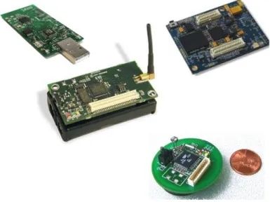
2.2 Wireless Sensors Examples . . . 7
2.3 WSN for Pipeline Security . . . 10
2.4 Environmental Monitoring Example . . . 11
3.1 CMUcam1, CMOS Based Camera . . . 15
3.2 CMOS Sensor Functioning Schema . . . 16
3.3 Spatial and Temporal Correlation Example. . . 18
4.1 Lossless Compression Schema . . . 28
4.2 Jpeg Compression Schema . . . 32
4.3 EZW Encoding Schema. . . 34
4.4 PRISM Encoding Schema . . . 38
4.5 DPCM Transmitter and Receiver Schema . . . 39
5.1 Intel Mote 2 . . . 42
5.2 IMB400 Module . . . 44
5.3 TinyViz Screenshot . . . 50
6.1 Camera GUI On Receipt Operations . . . 56
6.2 Run Length Encoding . . . 57
6.3 Example of a Shifted Picture . . . 59
6.5 Video Streaming Frames Sequences . . . 61
6.6 Video Coding Process . . . 62
6.7 Video Decoding Process . . . 63
6.8 Screenshot of the Gateway Side Application . . . 64
6.9 Video Packet Schema . . . 65
6.10 Interaction of Receiver and Display Threads . . . 66
7.1 Schemas of the Test Packets . . . 79
7.2 Picture Sample Used for Network Performances Monitoring . . . 80
7.3 Graph of the Transfer Times of a QVGA Picture . . . 81
7.4 Graph of Packets Retransmissions of a QVGA Picture. . . 82
7.5 Percentage of Retransmitted Packets in the Video Streaming System . 85 7.6 Percentage of Packets Lost in the Video Streaming System . . . 87
7.7 Graph of Buffer Emptying Times in High Motion Mode . . . 88
7.8 Graph of Buffer Emptying Times in Low Motion Mode . . . 89
7.9 Buffer Refilling Times in the Video Streaming System . . . 91
7.10 Resynchronization Time in the Video Streaming System . . . 93
7.11 Graph of The Simulated Sending Times of the Low Noise Simulation 95
List of Tables
5.1 CC2420 Power Levels . . . 43
7.1 Pictures Processing Times . . . 81
7.2 Video Processing Times. . . 84
7.3 Low Noise Simulation Results . . . 94
Chapter 1
Introduction
T
HEconsiderable scientific interest around Wireless Sensor Networks (WSN) of the past years was mainly due to the great potentialities of this kind of technology. WSNs offer a low cost and easily scalable network for data col-lection and environmental monitoring purposes. The price of this simplicity is payed in a resource constrained architecture presenting many limitations in terms of perfor-mance and functioning autonomy. These architectural limits give rise to a whole set of design issues faced by the scientific community in the last years: need to reduce en-ergy consumptions, reliability of the nodes, processing power of the motes, etc. Many research results have been reached allowing to extent the applications range of this technology from the original military context to other fields like environmental moni-toring, healthcare, data collection, etc.In the recent years, the technology progresses, in particular in image chips develop-ment, allowed to equip sensors with multimedia functionalities. Indeed, new CMOS based cameras reduce consistently the amount of energy required for image acquir-ing, maintaining a fair pictures quality. Such advances, together with the production of more powerful sensors and, at the same time, with reduced energy consumptions, extended further the fields of application of the WSNs in such a way that a new name was coined: Wireless Multimedia Sensor Network (WSNM).
WSNMs offer many new utilization possibilities that range from environments video monitoring, surveillance systems, patients monitoring, etc. But together with these new functionalities also new problems came. The processing efforts required by the multimedia contents strain also the new generation and most powerful sensors. More-over, such huge amount of data causes problem also in the transmission phase. Indeed, the network must sustain the increase of network traffic with related problems such as congestion and packets losses management. Together with this routing issues, the need of higher transmission rates and the long active periods of the radio chip bring not negligible energy consumption problems.
The developing of the video streaming system presented in this work had to take in account all these design issues. Before starting the software development, we did an accurate research on the current data compression techniques to evaluate whether one of them could perform better than the already implemented Jpeg encoder, for still images and to chose a light and efficient compression method to further reduce trans-mitted data size in the video subsystem.
The implemented work is based on an image acquisition software available among the Intel Mote 2 contributions developed by the Stanford University for TinyOS [3]. We exploited the original Jpeg compression algorithm implementation and the drivers of the OV7670 camera chip , installed on the IMB400 CrossBow multimedia module, to build a Difference Pulse Code Modulation (DPCM) algorithm to efficiently encode the video frames sequences. In a second phase the module for the serial communication with a general purpose computer, provided by the TinyOS contributions, has been ex-tended to support a reliable multihop radio protocol, based on the CC2420 chip drivers provided by the TinyOS 2.1.1 release.
The radio protocol implementation consisted in developing a sender module for the camera mote together with a base station attached to the general purpose machine. The base station has in charge to receive packets through the radio channel and to for-ward them to the gateway, on the serial connection. Moreover, we implemented the software supporting the insertion in the network of one or more intermediate nodes to
create a multihop network paradigm.
Also a Tossim simulation of the currently used network protocol has been imple-mented, as well as another losses management solution. This simulation was needed to compare such protocol with one of the most common alternatives, the Selective Repeatparadigm. Once the photo and the video subsystems, together with the radio protocol, were completed, the system performances were analyzed measuring image processing and network parameters. The different functionalities were tested varying the number of intermediate nodes, till a maximum of four, and the transmission power levels, going from 0 dBm to -25 dBm. The testbed preparation required some code modifications aimed to collect information without compromising the correctness of the measurements.
The outcome of the work will be deeply reported and explained in the rest of the dis-sertation:
Chapter2introduces the sensor networks describing the most important features and the most common applications.
In Chapter3, Wireless Multimedia Sensor Networks are analyzed also reporting the new challenges and issues deriving from this new sensor network paradigm.
Chapter4presents the results of the initial research work about the state of the art of images and video compression techniques.
In Chapter 6 we describe the design and development phases of the system deploy-ment. Moreover it is described the development of the network protocols simulation. In Chapter 7, the results of the performance tests for the different system configura-tions are presented.
Finally, in Chapter8considerations about the performances of the implemented system and the work outcomes are presented, together with possible future developments.
Chapter 2
Wireless Sensor Network
W
ireless sensor network (WSN) is a relatively new technology gaining a growing attention in the scientific and industrial community. This fact is referable to the diverse noteworthy and peculiar features offered by a sensor network, especially whether developed on a wireless architecture. A WSN, represented in Figure2.1, consists in a set of sensor nodes (also called motes) commu-nicating each others through a wireless channel, with no constraints on the topology of the network. Those sensors constitute a low cost and low power networked sys-tem, particularly well suitable to data collection and environment monitoring, easily adaptable to different aims through software programming. Moreover, this technology offers contained installation costs and a reduced maintenance. Examples of monitored data range from simple measurements, like temperature or humidity values, to more elaborated information, like accelerations or vibrations.The technological improvements in the hardware design of the last years have per-mitted to deal with sensors supporting a certain degree of on board computation and consuming a relatively small amount of energy; much help has come also from the large use of energy saving policies that involves network operations as well as the soft-ware executed by the sensor.
Figure 2.1: Schema of a WSN
The design of this kind of network is similar to the common ad-hoc networks planning methodology but with some differences, imputable to the distinct technology adopted: the number of nodes in a WSN can be notably higher than in an ad-hoc net-work, motes are densely distributed in the environment and the topology could change frequently. However, WSNs present new problems with respect a common wireless scenario: motes are largely exposed to malfunctions and are subjected to tight energy constraints. Though the network protocol has often been designed to maximize the energy savings communication is the activity with the highest energy dissipation in a generic WSN. Another issue comes from a common wireless network problem, that results amplified by the resource limits of the WSN: this is the low reliability of the wireless channel. While in a wired network the capacity of each link is fixed, in a wire-less environment, due to the interference level perceived at the receiver, the channel capacity can vary even consistently. Things get worse in a sensor network scenario, because transmission capacity is already limited and retransmissions cost energy.
2.1
Sensors
The typical hardware configuration of a mote consists of a micro controller for computation, a RAM memory to store dynamic data structures, flash memories where are placed the execution code and long-lived data, a communication module, composed of an antenna and a wireless transceiver, one or more sensors and a power source, usu-ally provided by batteries to support the versatility often required to this kind of net-work architecture. Some examples of currently available sensors are showed in Figure
2.2
It is possible to classify the sensing units in two separated categories: passive and ac-tive. While the first type of sensors does not need to act in an active manner to acquire information, like light and pressure transducers , the other one require a direct and constant action to acquire data, consuming a considerable amount of energy. This is the case, for example, of a sensor equipped with a camera.
One of the most famous motes is the MicaZ: it is based on an Atmel micro controller
Figure 2.2: Wireless Sensors Examples
log memory. On the communication side it has an IEEE 802.15.4 2.4-GHz transceiver that supports a maximum rate of 250 Kbps and a range of about 50 meters. It acquires data through a 10-bit ADC, and runs on two AA batteries. The processor current draw is of 8 mA in active mode while the radio frequency transceiver consumes almost 20 mA in receive mode.
2.2
Network
Inter node communication could be reached through different techniques. Infrared data transmission is tolerant to interference, offers reliable transmissions and is license-free but requires each node to be in line of sight with the others. Another approach exploits Bluetooth proprietary technology. The main issues of this solution are: high energy consumption, strong limitations on the number of nodes in the network and complex overlying MAC layer.
Many solutions bases the network communication on the IEEE 802.15.4 standard. The IEEE 802.15.4 standard was developed to provide a framework and the lower levels for low cost, low power networks. It only provides the MAC(Media Access Control) and PHY(PHYsical) layers, typically for a Personal Area Network (PAN), leaving the upper layers to be developed according to the market needs.
The chief requirements are low-cost, low-speed but ubiquitous communication be-tween devices. The concept of IEEE 802.15.4 is to provide communications over distances up to about 10 meters and with maximum transfer data rates of 250 Kbps. Additionally, when the hardware supports radio sleep mode, it permits to the recovered node a fast re-synchronization with the network.
2.3
Designing guidelines
To realize the typical WSN requirements, innovative mechanisms for a communi-cation network have to be found, as well as new architectures and protocol concepts. One of the main challenges is the need to support specific quality of service, lifetime and maintainability requirements of specific applications. On the other hand, these peculiar mechanisms also have to generalize to a wider range of applications allowing to contain costs.
The wireless medium adopted by these networks imposes the designer some limita-tions. In particular, communication between over long distances is only possible using prohibitively high transmission power. The use of intermediate nodes as relays can reduce the total required power. Hence, for many WSN implementations, multihop communication is a necessary solution.
The considerable number of nodes and the request of a simple deployment require the ability of the network to configure most of operational parameters autonomously, in-dependent with respect to external configuration. For example nodes should be able to determine their geographical position using only other nodes of the network. Also, the network should be able to tolerate failing nodes or to integrate new nodes.
In some applications, a single sensor is not able to decide whether an event has hap-pened but several sensors have to collaborate to detect an event and only the joint data of many sensors provides enough information. Instead of sending all the data to the edge of the network, where is processed, the information is elaborated in the network itself to achieve a collaboration model reducing the transmission load. An example could be the measurement of the average temperature in a place: while data are propagated through the network they are aggregated to reduce the total number of transmissions.
In a WSN, where nodes are typically deployed redundantly to protect against failures, the identity of the particular supplying data node becomes irrelevant. What is im-portant are the answers and the values themself, not which node has provided them.
Hence, the address-centric approach typical of traditional communication networks leaves room to a data-centric paradigm.
Another property required in a WSN is locality: nodes, who are very limited in mem-ory resources, should attempt to limit the state that they accumulate during protocol processing only to information about their direct neighbors. This help the network to scale to large numbers of nodes without having to rely on powerful processing at each single node.
Obviously, all these properties must be implemented in energy efficient manners, nec-essary to support long lifetimes.
2.4
Applications
WSN development was originally motivated by military purposes: this technology is particularly suitable in a war environment due of the fault tolerant characteristics and the self organizing capacity of the network. Furthermore, due to the low cost of
Figure 2.3: WSN for Pipeline Security
the components and the high mote density, the destruction of some devices does not affect the network integrity. Common uses include: battlefield surveillance, targeting and target tracking systems,nuclear, biological or chemical attack detection.
In the last years, WSN are gaining popularity even in a civilian context, where this science has found many fields of application, especially in environment monitoring
Figure 2.4: Environmental Monitoring Example
like, for example, precision agriculture,tracking of movements of small animals, pol-lution study. Two examples of WSN applications in a civilian context are showed in Figures 2.3 and 2.4. But WSN find space also in healthcare area, where this tech-nology is used in tracking and monitoring of patients as, for instance, in the Laura project [15], in drug administration in hospitals, providing interface for the disabled people etc. Others applications concern factory automation processes and smart home technologies.
Chapter 3
Wireless Multimedia Sensor Network
W
SN were originally focused on the collection of scalar data, simple pro-cessing and transmission to remote locations. Here, received data were processed by more powerful devices to obtain the most accurate infor-mation. More recently, the availability of inexpensive and low power hardware such as CMOS camera and microphones that allow to capture multimedia content from the environment has fostered the development of Wireless Multimedia Sensor Network (WMSN). These new devices allow retrieving video and audio streams, still images and scalar sensor data. In addition to the ability to collect multimedia data, WMSN are able to process, store and, in case of heterogeneous sources, correlate or fuse different information flows. This new research direction, not only enhance existing sensor net-work applications such as tracking, home automation, and environmental monitoring, but they will also enable several new ways of employment of this kind of technology:• Multimedia surveillance sensor network:
wireless video sensor networks will be composed of interconnected, battery-powered miniature cameras, each packaged with a power wireless transceiver capable of processing, sending and receiving data. Video and audio sensors will be used to complement existing surveillance systems.
Multimedia sensors could infer and record potentially relevant activities (thefts, car accidents, traffic violations), and make video/audio streams reports available for future query.
• Traffic avoidance, enforcement and control systems:
it will be possible to monitor car traffic in big cities or highways and deploy services that offer traffic routing advice to avoid congestion or simply to collect vehicular traffic data.
• Advanced health care delivery:
Patients will carry medical sensors to monitor parameters such as body temper-ature, blood pressure, pulse oximetry, ECG, breathing activity. Furthermore, remote medical centers will perform advanced remote monitoring of their pa-tients via video and audio sensors, location sensors, motion or activity sensors, which can also be embedded in wrist devices.
• Automated assistance for the elderly and family monitor:
Multimedia sensor networks can be used to monitor and study the behavior of elderly people. Networks of wearable or video or audio sensors can infer emer-gency situations and immediately connect elderly patients with remote assis-tance service or relatives.
• Environmental monitoring:
Several projects on habitat monitoring that use acoustic and video feeds are being envisaged. For example, arrays of video sensors are already used by oceanographers to determine the evolution of sandbars via image processing techniques[10]].
• Person locator services:
Multimedia content such as video streams and still images, along with advanced signal processing techniques, can be used to localize missing people, or identify wanted criminals.
• Industrial Process Control:
Imaging, temperature and pressures for instance, may be used for time-critical industrial process control. For example, in quality control of manufacturing pro-cesses, such as those used in semiconductor chips, automobiles, food or phar-maceutical products.
3.1
Multimedia sensors
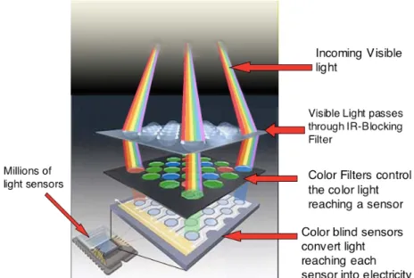
Figure 3.1: CMUcam1, CMOS Based Camera
A multimedia sensor does not differ much from common sensors, as those exam-ined in Chapter2. Basically they are equipped with a processing unit, a communication subsystem, a coordination system and a storage unit. The great difference is the multi-media module and the correspondent analog-to-digital (ADC) converter. Usually this module is equipped with a microphone but, most of all, an image sensor as the one showed in Figure3.1. This add new capacities to the mote but increases also the com-plexity of some components such as the ADC. Since 1975 till few years ago, the de
facto standard for image sensors was the CCD (charge coupled device). As compared to traditional CCD technologies, there is a need for smaller, lighter camera modules that are also cost-effective when bought in large numbers to deploy a WMSN.
In a CCD sensor, the incident light energy is captured as the charge accumulated on a pixel, which is then converted into a voltage and sent to the processing circuit as an ana-log signal. This architecture brings some disadvantages with respect to its integration on a wireless sensor: they require more electronic circuitry outside the actual image sensor, are more expensive to produce and, above all, they consume up to 100 times power than a CMOS sensor. Unlike the CCD sensor, the CMOS chip incorporates
am-Figure 3.2: CMOS Sensor Functioning Schema
plifiers and A/D-converters, which lowers the cost for cameras since it contains all the logics needed to produce an image. Every CMOS pixel contains conversion electron-ics. Compared to CCD sensors, CMOS sensors have better integration possibilities and more functions. However, this addition of circuitry inside the chip can lead to a risk of more structured noise, such as stripes and other patterns. CMOS sensors also have a faster readout, lower power consumption, higher noise immunity, and a smaller
system size[11]. In Figure3.2 it is showed how the CMOS sensor captures the image transforming it in an electrical signal. Depending upon the application environment, such as security surveillance needs or biomedical imaging, these sensors may have different processing capabilities.
3.2
Design Issues
The volume of data collected as well as the complexity of the necessary in-network stream content processing provides a diverse set of challenges in comparison to generic scalar sensor network research. Multimedia motes have to support tasks increasingly demanding in terms of number and computational complexity of operations. Due to the considerable energy dissipation spent in transmission, acquired data have to be elaborated in order to reduce size. This task could require a lot of energy resources if low complexity and efficient coding techniques are not used. Moreover, acquiring more and more accurate data, increase dramatically the load in the entire network. For this matter, it is necessary, to combine data compression techniques with new trans-mission policies aimed at reduce the network traffic.
The wide variety of applications envisaged will have different requirements. In addi-tion to data delivery modes typical of scalar sensor networks, multimedia data include content based requirements. This force to consider QoS (Quality of Service) and ap-plication specific requisites. These requirements may pertain to multiple domains and can be expressed, amongst others, in terms of a combination of bounds on energy con-sumption, delay, reliability, distortion, or network lifetime.
Multimedia contents, especially video streams, need transmission bandwidth that is orders of magnitude higher than that supported by currently available sensors. For ex-ample, the nominal transmission rate of state-of-the-art IEEE 802.15.4 is 250 Kbit/s. Data rates at least one order of magnitude higher may be required for high-end multi-media sensors, with comparable power consumption. Therefore we need to balance the trade-off between transmission performance and energy consumption. A help could
come from new transmission techniques such as UWB (Ultra Wide Band)[4]
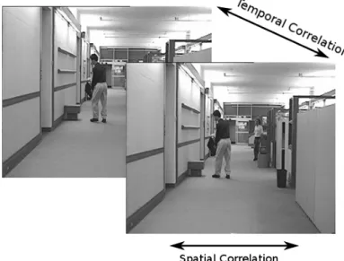
Because of the considerable amount of data generated by multimedia sensors, efficient processing techniques for lossy compression are necessary for this kind of networks. Traditional video coding methods are based on reducing bits generated by the source encoder by exploiting the source statistics. More commons encoders rely on intra-frame compression techniques to reduce the redundancy within the same intra-frame and inter-frame compression to exploit redundancy between subsequent frames. The two correlation types are showed in Figure 3.3. Since predictive (inter-frame) coding
re-Figure 3.3: Spatial and Temporal Correlation Example
quires powerful processing algorithms it may not be suited for low-cost multimedia sensors. The solutions adopted try to move as much computation as possible to the decoder, designing lightweight and distributed source encoders that produce different small data flows put together by the decoder [9].
WMSN allow performing multimedia in-network processing algorithms on the raw data extracted from the environment. This requires new architectures for collaborative, distributed and resource constrained processing that allow for filtering and extraction of semantically relevant information at the edge of the sensor network. In this way it,
is possible to increase the system scalability by reducing the transmission of redundant information, merging data originated from multiple views, on different media and with multiple resolutions.
Obviously power consumption has a central role in the deployment of WMSN. The considerable amount of data and its elaboration require energy saving oriented algo-rithms, even more than in traditional WSN. In fact, while the energy consumption of traditional sensor nodes is known to be dominated by the communication facilities, it may not necessarily be true in WMSN.
Wireless multimedia sensor networks will support several heterogeneous and indepen-dent applications with different requirements. It is necessary to develop flexible, hier-archical architectures that can accommodate the requirements of all these applications in the same infrastructure.
3.3
State Of The Art
The field of video sensor networks is a relatively new area of interest that offers different research opportunities. The add of multimedia content to the sensor networks required a rethinking of the network layers and architecture. Many of the last years re-searches were focused on answering to the requirements of the new network paradigm. With the increase of the required bandwidth, the old MAC (Medium Access Control) protocols became inefficient. Indeed, existing schemes are based mostly on variants of CSMA/CA (Carrier Sense Multiple Access, with Collision Avoidance) MAC protocol and present notable limitations in terms of latency and coordination complexity. The channel contention could be significantly reduced using two radios in which to one is delegated the task of channel monitoring and is responsible for waking up the main ra-dio for data communication. The disadvantages of this approach reside in the distinct channels assignment and in the increased hardware complexity.
A contention free alternative could be the implementation of a TDMA (Time Divi-sion Multiple Access) protocol. With this paradigm, channel resources are assigned
in a small time interval with a contention based method while the rest of the frame is contention-free and divided on the basis of the QoS (Quality of Service) requirements. The main problems of this technique concern the network scalability and the complex network-wide scheduling.
A third way reproduces MIMO (Multiple Input Multiple Output) antenna systems, where each sensor functions as a single antenna, sharing information and simulating a multiple antenna array.
The unreliability of the wireless channel requires error correction mechanisms. The main link layer classes of error correction protocols are FEC (Forward Error Control) and ARQ (Automatic Repeat Request). While the former applies different degrees of redundancy to different parts of the video stream, on the basis of the part importance, the ARQ protocols use the bandwidth efficiently at the cost of additional latency in-volved with the retransmission process. Recent comparisons between the two tech-niques showed that for certain FEC block codes (BCH), longer routes decrease both the energy consumption and the end-to-end latency [21].
In a WMSN could exist nodes with different capabilities. Consequently there could be different routes with different characteristics based on the diverse features of the nodes along the path. Moreover the routing could be based on video stream content. For instance, streams belonging to cameras with the same orientation could follow the same route to facilitate redundancy removal.
Another approach could speed up the routing procedures differentiating between flows with different delay and reliability requirements. Each node selects its next hop based on link-layer delay measurements [8].
Transport layer protocols can follow UDP (User Datagram Protocol) or TCP (Trans-port Control Protocol) models. Usually, for multimedia contents, UDP paradigm is more appreciated. It allows to give more importance to timeliness constraints than reliability requirements. The Real-time Transport Control Protocol (RTCP), based on UDP, permits a dynamic adaptation to the network conditions, allowing bandwidth scaling and integration of different images in a single composite. In addition, with
application level framing (ALF) it is possible to ensure a better compatibility between different networks, such as WSN and IP-networks, encoding specific instructions in the packets header.
On the other side, TCP approaches support a more selective management of the net-work traffic. For example, in MPEG protocol, some frames, called I-frames, can not be retrieved by interpolation and dropping packets indiscriminately, as in the case of UDP, may cause discernible disruptions in the multimedia content. It would be better to introduce a sort of selective reliability mechanism that increases the protection of these packets with respect to less important parts.
Although many of the cited works were developed in a simulated environment, some of them were implemented. For example in the surveillance systems, where WMSN allow costs reduction and more flexibility in the system installation, new way of mon-itoring are offered, like target classification and tracking [7].
Alongside of the existent development environments, new frameworks are developed with the aim of helping the designers in implementing new multimedia applications that can exploit the potentialities offered by sensors with multimedia capabilities [16]. The increase of the network traffic, due to the multimedia content of the network, re-quires the developing of new routing protocols to efficiently drain the huge amount of data. Older protocols must be updated or substituted by newer and more reliable traffic management methods [19].
Other research studies concern testbeds to test new protocols and applications devel-oped for Wireless Multimedia Sensor Networks or to measure how the existent tech-niques perform with respect to the new and more problematic multimedia approaches [13].
Chapter 4
Image Coding Techniques
T
HE considerable amount of information produced by a multimedia sensor together with the limited resources of commons WSN, require data com-pression techniques to reduce the network load and the intermediate node’s processing efforts.Images are made of pixels, each pixel is described by a variable number of bits de-pending on the image type, grayscale or colored, and quality. The number of bits re-quired to represent an image may be substantially lower because of redundancy. This redundancy can be classified in three different types: spatial redundancy, due to the correlation between neighboring pixel values, spectral redundancy, generated by the correlation between different color planes or spectral bands and temporal redundancy, due to the correlation between different frames in a sequence.
Image compression research aims to reduce the number of bits required to represent an image by removing these redundancies.
The most general categories in which a compression method could fall are: lossless and lossy compression. While lossless methods allow to reconstruct an image identical to the original, on a pixel-per-pixel base, lossy compression drops some information with respect to the original, so that the result of reconstruction operations contains degradations.
In a WMSN environment, the choice of a technique aimed to reduce the size of an image captured by a node must be driven by the performance limits of the mote’s hardware and by the energy constraints to which it is subjected.
The major part of compression techniques elaborate the signal transforming it and pro-cessing data in frequency domain to exploit properties of the transform with the aim of a more efficient compression of the information.
4.1
Fourier Transforms
There exist many types of transforms: Fourier, Cosine, Hadamard, Karhunen Lo-eve, Tchebichef, etc. Each one has different properties and complexity. In the image compression field discrete Fourier transformation (DFT) is frequently used because it can condense most of the image information in few coefficients. The main issue is the high computational complexity. On the other side, Hadamard transformation is very fast and performs better than Tchebichef or discrete cosine transformation (DCT) with images containing rapid gradient variations while loses effectiveness for continuous tone images[12].
One of the most used transforms, adopted in JPEG and MPEG standards, is DCT. This technique is used when the input signal contains only real parts: it is referable to the Fourier transform where the the imaginary part is always zero. It is appreciated for the compromise between performance and effectiveness offered and for some owned properties like the fact that for real inputs it gives real output so that less storage space is needed and for the ability of exploiting the correlation between adjacent pixels. DCT is able to concentrate most of the signal in the lower spatial frequencies so that, in the subsequent quantization operations, most of high frequencies coefficients have a zero or negligible value and can be cut. Another advantage of the DCT is the possibility of computing the transform with a reduced complexity. Although the direct application of these formulas would requires O(N2) operations, it is possible to compute the same
thing with only O(NlogN) complexity by factorizing the computation similarly to the fast Fourier transform (FFT) [6].
The DCT represents a finite set of points in a sum of cosine functions,oscillating at different frequencies.
The one dimension DCT formula is:
n
∑
0 xncos[ π N(n + 1 2)k] k= 0, ..., N − 1 (4.1)For image processing, which obviously deal with two dimensions arrays, it is suf-ficient to apply such transformation two times.
Consider a signal X of size M by N. Then the 2D DCT of X is given by Y which is also a M by N signal, where Y is given by:
Ypq= αpαq M−1
∑
m=0 N−1∑
n=0 Xmncos(π 2m + 1 2M p)cos(π 2n + 1 2N q) (4.2) αp= 1 √ M i f p== 0 2 √ M else αq= 1 √ N i f q== 0 2 √ N elseThe purpose of the transformation is to prepare the data set for the compression. The output of the DCT algorithm contains the same information of the original image, it is a lossless step. Usually this transformation is followed by two others elaborations: quantization and entropy encoding. These will be examined in details in the next para-graphs.
4.2
Wavelets
The Fourier transform is only able to retrieve the global frequency content of the signal, while the time information is lost. This is overcome by Short Time Fourier Transform (STFT) which, applying a constant temporal window in the calculation of
the Fourier transform, can retrieve also temporal information. Notice that, due to the fixed window length, they are extracted constant-time and constant-frequency reso-lution samples. This works well for low frequencies where often a good frequency resolution is required over a good time resolution while, for high frequencies, time resolution is more important than frequency resolution.
The wavelet transform allows a multi-resolution analysis. It is calculated similarly to the Fourier transform but trigonometric analysis functions are replaced by a wavelet function. A wavelet is a short oscillating function that contains both the analysis func-tion and the window. Time informafunc-tion is obtained by shifting the wavelet over the signal while the frequencies are changed by contraction and dilatation of the wavelet function.
The discrete wavelet transform (DWT) is gaining increasing importance in digital im-age processing. It uses filter banks to perform the wavelet analysis. The DWT trans-form decomposes the signal into wavelet coefficients from which the original signal can be reconstructed again. The wavelet coefficients represent the signal in various frequency bands. The coefficients can be processed in several ways, giving the DWT attractive properties over linear filtering.
The DWT is defined as:
C( j, k) =
∑
n∈Z f(n)ψjk(n) (4.3) where ψjk(n) = 2− j 2ψ(2− jn− k)Images are analyzed and synthesized by bi-dimensional filter banks. The low frequen-cies, extracted by high scale wavelet functions, represent flat background, the high frequencies represent regions with textures. The compression is performed with a multi level filter bank that divides the signal in subbands. Lower bands, that give an approximation of the original image and are supposed to last for the entire duration of the signal, must be codified with less bits whereas higher frequencies, that represent image details and are assumed to appear from time to time, should have fewer bits.
After the DWT analysis, bit allocation and quantization is performed on the coeffi-cients. The coefficient are grouped scanning and coded for compression. The process of entropy coding can be split in a modeling part where probabilities are assigned to the coefficients and a coding part where each coefficient is coded. An image could be compressed also ignoring coefficient under a threshold to obtain lossy compression. This technique finds application also in video compression.
4.3
Image Compression Algorithms
There is a considerable number of compression techniques in literature. As for transforms algorithms each one has peculiar advantages and disadvantages. It is not in the purposes of this work to discuss all the existent methods, therefore only some of them will be taken in account in order to give an idea of the diverse approaches that can be used in image processing.
4.3.1
Lossless compression
Lossless compression algorithms allow the reconstruction of the exact original data set starting from compressed data. This kind of compression is used in many appli-cations such as ZIP or GZIP file formats. It is mainly adopted for text or source code compression or in specific image format such as PNG or GIF. All the lossless com-pression techniques rely on Shannon’s noiseless coding theorem [18] that guarantees the correct decoding of the compressed data as long as the average number of symbols out of the decoder exceeds the source entropy by an arbitrary small amount.
As showed in Figure 4.1, almost all lossless compression methods consist of two stages: decorrelation and entropy coding. Decorrelation means remove the redun-dancies present in the original data source while entropy coding consists, basically, in assigning smallest codewords to more frequent source symbols.
employed especially in grayscale images coding. This method considers the binary representation of each pixel and builds as many matrixes as the number of bits that constitute the pixel word, filling each matrix with bits that covers the same position in the different words (bit planes). Each bit-plane is then separately compressed using run-length encoding.
Decorrelation
s(n) Entropy Coding x(n)
Figure 4.1: Lossless Compression Schema
Decorrelation
One noteworthy decorrelation technique is linear prediction. It consists basically in a differential pulse code modulation (DPCM) without quantization. For each sample it builds a prediction from the weighted sum of neighboring samples. Decorrelation is accomplished subtracting predictions to the actual sample values so that the entropy of the source results diminished.
Another decorrelation method is associated to transforms. Since to avoid losses we can not apply quantization, the approach consist in coding the information otherwise discarded. This is accomplished subtracting the output of the lossy coder (transforma-tion and quantiza(transforma-tion) from the original data set and entropy coding the result. It must be said that this coding technique does not reach a noteworthy compression ratio. Alongside of these technologies there is a set of multi resolution techniques includ-ing hierarchical interpolation (HINT), the Laplacian pyramid and the S-Transform. These methods form a hierarchy of data sets representing the original data with vary-ing resolution and supportvary-ing therefore progressive transmission which allows data to be decoded in several stages. For example, HINT starts with a subsample version of the original data set that has been coded with any lossless technique. Linear prediction
is then applied to subsampled data to estimate intermediate samples. Subsequently the difference between estimated intermediate sample and actual intermediate samples is entropy coded. The process is repeated until all the intermediate samples have been estimated.
Entropy Encoding
The probability mass function (PMF), in probability theory, is a function that gives the probability that a discrete random variable assume a certain value. Unless the PMF of the decorrelated data is uniform, entropy coding can be applied to further compress the data. The majority of compression schemes employ Huffman coding or arithmetic coding.
Huffman coders generate, given a source alphabet and the corresponding PMF, the optimal set of variable length binary codewords of minimum average length. The Huffman codes length is always within one bit of the entropy bound. Most practical Huffman encoders are adaptive and estimate the source symbols probabilities from the data. A Huffman code is built in such a way that a word can not be a prefix of another word and that words with highest number of occurrences are coded with shorter code-words.
Arithmetic coding is a generalization of Huffman coding. The principle is the same as Huffman coding: it is a variable length encoding scheme where frequently used characters will be stored with fewer bits. Rather than separate the input into compo-nent symbols replacing each with a codeword, the arithmetic encoding codes all the message in a single number, a fraction n where 0.0 < n < 1.0. The decoding process start dividing the real interval [0.0, 1[ in subintervals corresponding to the PMF of the symbols. In this way exists a direct relation between an interval and a source alphabet symbol. The first decoded word is found looking up in which interval the received number falls. Then the individuated interval is subdivided in the same manner as be-fore and the procedure is recursively repeated until all the message has been decoded.
The Lempel-Ziv-Welch (LZW) coder was developed for text compression but was also applied in signal compression with limited success. It is a dictionary based technique: when a sequence of symbols matches a word stored in the dictionary, its index is sent, otherwise the sequence is forwarded without coding and is subsequently added to the dictionary. This algorithm does not need to be preceded by decorrelation procedures because exploits source correlation. The main issue of this method is that the dictio-nary size increases rapidly with increasing sample resolution, making it unsuitable for high performance applications.
Another frequently used technique is the run-length coding, particularly useful for compression of binary source data where long sequences of the same symbol have high probability. The idea at the ground of this method is to transmit the length of the runs of repeated symbols instead of transmitting each symbol.
4.3.2
Lossy compression
Lossy compression is a data encoding method in which some information is de-liberately discarded to achieve a better compression ratio. This methods are mainly applied in the discretization of continuous sources in a finite set of discrete values but find also employment in the transformation of a discrete source in another with a smaller alphabet. Obviously the applying of this techniques introduce a distortion in the resulting output signal. This degradation is usually quantified through dedicated metrics that, with the reached compression ratio (the ratio between compressed size and original size), is used to estimate the fairness of the algorithm.
Quantization
Quantization is the non invertible operation used to discretize a set of continu-ous random variables. It can be distinguished in: scalar quantization, referred to the quantization of a single random variable, and vector quantization, referred to the quan-tization of a block of random variables simultaneously. Moreover, it can be applied
to already discrete sources to obtain a coarser representation of the original data set which allows the possibility of higher compression ratios. The method is based on a set of output values, called reproduction levels, and on a set of decision regions stated with the constraint that each one of the source symbols belongs to one interval. The quantization function substitutes each value of the source with the corresponding re-production level. In this way the initial alphabet is reduced to a smaller set of symbols. Vector quantization is the generalization of the scalar quantizer of a single variable to the case of a block or a vector of random variables. Augmenting the samples length increases the coding capacity because the simultaneous coding of a group of random variables allows a more efficient representation of the source information. The func-tioning is the same for the single variable case but here the decision regions are in Rn. The design of an optimal generic quantizer for a source with given statistics, con-sists in finding the codebook and the partition that minimize the distortion. There are different optimization methods: for scalar quantizer it is often used the Lloyd-Max algorithm from which it has been derived the Linde-Buzo-Gray (LBG) algorithm for vector quantizers.
Jpeg
Jpeg is the acronym for Joint Photographic Expert Group. It has published diverse standards for image compression: among those we mention Jpeg, lossy compression algorithm of continuous tone still images, Jpeg-LS, lossless and near lossless com-pression algorithm for continuous tone still images and Jpeg2000, scalable coding of continuous tone still images, lossless and lossy.
The most famous of them, Jpeg, has been developed in different implementations. The baseline version of the standard includes the following phases: each color component is divided in blocks of 8x8 pixels each, then each block is processed independently applying DCT transform, subsequently the output of the DCT step is quantized cutting off the transform coefficients with a value minor than a threshold. At last the data flow
is run length and Huffman encoded. The quantization step could be influenced tuning the quality factor of the Jpeg algorithm: this number is usually comprised between 0 and 100 and its value is inversely proportional to the quality of the output image. A schema of the Jpeg compression steps is showed in Figure4.2.
The Jpeg standard is appreciated for its low complexity, the limited memory require-ments and the reasonable coding efficiency. On the other side it presents also many issues such as blocking artifacts at low bit rate, does not have lossless capabilities, poor error resilience etc.
Some of the problems have been fixed in the Jpeg2000 standard. Here we find an im-proved coding efficiency, full quality scalability from lossless to lossy at different bit rates, division of the image in subimages (tiling), improved error resilience and region of interests, part of the image that can require a better quality compression. Another interesting characteristic in Jpeg2000 standard is the use of wavelet transformation in place of the discrete cosine transformation. This brings consistently advantages in scalability management: while in Fourier transformations, to which DCT belongs, the basis functions cover the entire signal range, varying in frequency only, wavelet basis functions vary in frequency as well as spatial coordinate. This allow to achieve spa-tial scalability reconstructing from only low resolution coefficients as well as quality scalability decoding only sets of bit planes, starting from the most significant bit plane.
DCT 8x8
Blocks Quantization
Entropy Encoding
CodedStream Run LengthEcoding
Embedded Zerotree Wavelet and Set Partitioning in Hierarchical Trees
An embedded coding is a process of encoding the transform coefficients that allows for progressive transmission of the compressed image. Zerotrees are a concept that al-lows for a concise encoding of the positions of significant values that result during the embedded coding process. The embedding process used in EZW is called bit-plane encoding. The EZW algorithm is specially designed to use with wavelet transforma-tion.
The method is divided in multiple steps, showed in Figure4.3. First of all it must be chosen the threshold value, so that there exist at least one wavelet coefficient greater than the threshold. Subsequently, the threshold value is halved and then, in the sig-nificance pass, the algorithm builds the set of wavelet quantized coefficients assign-ing wq= Tk and sending in output the coefficient sign whether the absolute value of
the correspondent wavelet coefficient is greater than the threshold, otherwise leav-ing wq= 0. In the refinement pass the algorithm scans through significant values: if
w(m) ∈ [wq(m), wq(m) + Tk] it outputs the bit 0, if w(m) ∈ [wq(m) + Tk, wq(m) + 2Tk]
it outputs the bit 1.
In few words, the bit-plane encoding of the EZW algorithm consists in computing bi-nary expansions for the transform values using the initial threshold as unit and then recording in magnitude order only the significant bits of these expansions. During the decoding process the signs and the bits output can be used to reconstruct an approxi-mate wavelet transform to any desired degree of accuracy. Once obtained the desired detail level, it is possible to decide to stop the decoding process.
Zerotrees are exploited to reduce the number of bits sent to the decoder. It must be noticed that natural images in general have a low pass spectrum. When an image is wavelet transformed the energy in the subbands decreases as the scale decreases (low scale means high resolution), so the wavelet coefficients will, on average, be smaller in the higher subbands than in the lower subbands. Moreover, large wavelet coefficients are more important than smaller wavelet coefficient. There are coefficients in different
Coded Stream Bit -Plane Encoding
Significant Pass Refinement Pass Wavelet Transform Arithmetic Encoding Zerotree Location Input Stream
Figure 4.3: EZW Encoding Schema
subbands that represent the same spatial location in the image and this spatial relation can be depicted by a quad tree except for the root node at top left corner representing the DC coefficient which only has three children nodes. A quad tree is defined as a tree of locations in the wavelet transform. If the tree root is in [i,j] its children are located at [2i,2j], [2i+1,2j], [2i, 2j+1] and [2i+1,2j+1]. A quad tree can have multiple levels when a child is the root of another tree.
A zerotree is defined as a quad tree which, for a given threshold T, has insignificant wavelet transform values at each of its locations.
Once wavelet coefficient have been encoded, with respect to the current threshold, in ones (higher than T) and zeros (lower than T), the EZW exploits the zerotrees based on the observation that wavelet coefficients decrease with scale. It assumes that there will be a very high probability that all the coefficients in a quad tree will be smaller than a certain threshold if the root is smaller than this threshold. In this case the whole tree can be encoded with the zerotree symbol. Fortunately, with wavelet transform of natu-ral scenes, the multi resolution structure of the wavelets does produce many zerotrees allowing to reduce notably the compressed data size. After identified the zerotrees, the data are encoded using an arithmetic encoding algorithm.
version of the EZW. It offers highest PSNR (Pixel Signal Noise Ratio) for given com-pression ratios, consequently it is probably the most widely used wavelet algorithm for image compression. Set partitioning refers to the way these quadtrees divide up, partition, the wavelet transform values at a given threshold. The analysis of this parti-tioning of transform values has been exploited to improve EZW algorithm.
SPIHT makes use of three lists: the List of Significant Pixels (LSP), List of Insignif-icant Pixels (LIP) and List of InsignifInsignif-icant Sets (LIS). These are coefficient location lists that contain their coordinates. After the initialization, the algorithm takes two stages for each level of threshold: the sorting pass (in which lists are organized) and the refinement pass (which does the actual progressive coding transmission). The re-sult is in the form of a bitstream.
SPHIT uses a state transition model to encode zerotree information. Every index in the baseline scan order is assigned to a state depending on its value with respect the current threshold and the output of a significant function. From one threshold to the next the locations of transform values undergo state transitions. State transitions are coded with a smaller amount o¡f bits with respect the whole states: the states are four and only from one state all the others can be reached; the second and the third state can reach only two states while the last state is final. Encoding only the state transitions allows SPHIT to reduce the number of bits needed.
This algorithm performs better than other more sophisticated algorithms. For example it outperforms Jpeg both in perceptual quality and in terms of PSNR. Moreover it is less exposed to artifacts. It also is more efficient and more effective than EZW [17].
4.4
Video Compression Algorithms
Today’s digital video coding paradigm represented by the ITU-T and MPEG stan-dards mainly relies on a hybrid of block based transform and interframe predictive coding approaches. In this coding framework, the encoder architecture has the task to exploit both the temporal and spatial redundancies present in the video sequence,
which is a rather complex exercise. As a consequence, all standard video encoders have a much higher computational complexity than the decoder (typically five to ten times more complex), mainly due to the temporal correlation exploitation tools, notably the motion estimation process. This type of architecture is well-suited for applications where the video is encoded once and decoded many times, i.e., one-to-many topolo-gies, such as broadcasting or video-on-demand, where the cost of the decoder is more critical than the cost of the encoder. On a sensor network the encoders have limited processing capacities while the decoders usually are run on machines out of the sensor network that can face major computational complexities.
Distributed Video Coding
The emerging technology for video streaming processing on wireless sensor net-works is the Distributed Video Coding (DVC). The signals are captured independently by different sources and subsequently merged by a central base station that has the capability to jointly decode them.
The theoretical foundation of this technology can be found in the Slepian-Wolf coding theorem. It establishes that, if two sources are coded separately, provided that they are decoded jointly and that their correlation is known to both the encoder and the decoder, the lossless compression rate bound represented by the joint entropy H(X,Y) can be approached with a vanishing error probability[20]. Another contribution was given by Winer-Ziv studies. They showed that for correlated Gaussian source and a mean square error distortion measure, there is no rate loss in the independent coding of the sources with respect to the joint coding and decoding of the two sources [22]. One of the first applications in DVC is PRISM, by the Berkeley’s group [14]. The algorithm divides the stream in group of pictures on which a complete cycle of coding decoding process is applied. The first frame of this group of pictures is encoded in a traditional way, for example with AVC/H.264 Intra [5]. This first frame is then used
to encode the remaining frames of the group with an hybrid technique, showed in Fig-ure4.4which combines distributed and traditional coding. Each frame is split in 8x8 blocks and then transformed. Each block is considered as a separate unite and encoded independently from its spatially neighboring blocks. Then, the encoder estimates the current block’s correlation level with the previous frame by using a zero-motion block matching. Further the blocks are classified into different encoding classes depending on the level of estimated correlation. The blocks with a lower level of correlation are encoded using conventional coding methods while high correlated blocks are not coded. The medium correlation blocks are encoded with a distributed approach where the number of bits used depends on the correlation level. The encoder computes syn-drome bits used, at decoder side, to correct different predictors.
Another implementation is called Stanford codec. Video sequence is again split in groups of pictures: the first picture of the group is called key frame and is coded with traditional methods. The remaining frames are completely encoded in a distributed fashion passing through a quantization phase and then Turbo encoded. At decoder side intermediate frames are decoded by interpolation between the key frames. The decoder corrects its prediction using parity bits received from the encoder.
Interframe Video Compression
Interframe compression includes those techniques applied to a sequence of video frames and not only within an image. Interframe compression exploits the similarities between successive frames, known as temporal redundancy, to reduce the volume of data required to describe the sequence.
The most established and implemented strategy is the block based motion compensa-tion technique, employed in MPEG or ITU-T video compression standards. This tech-nique is based on motion vector estimation: the image is divided into disjoint blocks of pixels and each block is compared to areas of similar size of the previous frames to find an area that is similar. A block from the current frame for which a similar area is
8x8 Block
DCT
Esteem of the Block Correlation
High Medium Low
Distributed Coding Not Coded Conventional Coding Methods Syndrome Generation
Figure 4.4: PRISM Encoding Schema
sought is known as a target block. The location of the similar or matching block in the past frame might be different from the location of the target block in the current frame. The relative difference in locations is known as the motion vector. If the target block and matching block are found at the same location in their respective frames then the motion vector that describes their difference is known as a zero vector. In the coding phase, instead coding blocks that simply moved through the image, the encoder codes the motion vectors describing such a movement. During decompression the decoder uses the motion vectors to find the matching blocks in the past frame and copies those blocks in the right position.
The effectiveness of compression techniques that use block based motion compensa-tion depends on some assumpcompensa-tions: objects move on a plane that is parallel to the camera plane, illumination is spatially and temporal uniform and occlusion of one ob-ject by another does not happen.
Another interesting technique often adopted for its simplicity is Differential Pulse Code Modulation(DPCM). This coding system merges predictive coding and scalar
quantization. The technique exploits the correlation between two subsequent frames coding the prediction residual. This residual, due to inter-symbol correlations assumes small values with high probability, thus having a smaller variance than the source. With continuous signals this small variance allow to reduce the quantization error variance, that is proportional to the variance of the quantizer input. Moreover it is possible to design adaptive quantizers that compensate slowly varying input signal power by dy-namically scaling the quantizer output.
DPCM is also suitable for discrete signals as video sequences. The basic idea ex-ploits again the correlation between closest frames but this time predicted residuals have not to be quantized. The residual coefficients are zeros or near zeros values and constitute the ideal input for the subsequent compression phases as, for instance, transforms and run length coding. Due to the proximity and the smallness of those values the mentioned techniques can achieve better compression results exploiting the reduced amount of information carried by the data set. A schema of the DPCM en-coder/decoder is showed in Figure4.5.
Decoder Predictor Channel
Receiver
Quantizer Predictor Coder Original Image Channel + +-Transmitter
+ Reconstructed ImageChapter 5
Hardware and Software
I
N this Chapter the hardware and software components used to implement the video streaming on the sensor network will be presented in details.An accurate analysis of the hardware features of the adopted sensors was neces-sary for the developing of the entire system. Quality parameters and performances of the components had to be considered to avoid bottlenecks and to tune properly all the variables involved.
5.1
Crossbow Intel Mote 2
The Intel Mote 2, Figure 5.1, is an advanced sensor network node platform de-signed for demanding wireless sensor network applications requiring high CPU/DSP and wireless link performance and reliability.
The platform is built around a low power XScale processor, PXA271. It integrates an 802.15.4 radio (ChipCon 2420) and a built in 2.4 GHz antenna. It exposes a “basic sensor board” interface, consisting of two connectors on one side of the board, and an “advanced sensor board” interface, consisting of two high density connectors on the other side of the board. The Intel Mote 2 is a modular stackable platform and can be stacked with sensor boards to customize the system to a specific application, along
with a “power board” to supply power to the system.
Figure 5.1: Intel Mote 2
Processor
The Intel Mote 2 contains the PXA271 processor. This processor can operate in a low voltage (0.85V) and a low frequency (13 MHz) mode, hence enabling low power operation. The frequency can be scaled to 104 MHz at the lowest voltage level, and can be increased up to 416MHz with Dynamic Voltage Scaling (DVS). Currently DVS is not supported by TinyOS 2.x and the voltage level can only be set to 13, 104 or 208 MHz. The processor has many low power modes, including sleep and deep sleep modes. It also integrates 256 KB of SRAM divided into 4 equal banks of 64 KB. The PXA271 is a multi-chip module that includes three chips in a single package, the processor, 32 MB SDRAM and 32 MB of flash. The processor integrates many I/O op-tions making it extremely flexible in supporting different sensors, A/Ds, radio opop-tions, etc. These I/O options include I2C, 3 Synchronous Serial Ports one of which dedicated to the radio, 3 high speed UARTs, GPIOs, SDIO, USB client and host, AC97 and I2S audio codec interfaces, fast infrared port, PWM, Camera Interface and a high speed bus (Mobile Scaleable Link). The processor also adds many timers and a real time clock. The PXA271 also includes a wireless MMX coprocessor to accelerate
multi-media operations. It adds 30 new multi-media processor instructions, support for alignment and video operations and compatibility with Intel MMX and SSE integer instructions.
Radio
The Intel Mote 2 integrates an 802.15.4 radio transceiver from ChipCon (CC2420). 802.15.4 is an IEEE standard describing the physical and MAC layers of a low power low range radio, aimed at control and monitoring applications. The CC2420 supports a 250 kb/s data rate with 16 channels in the 2.4 GHz band. The Intel Mote 2 platform integrates a 2.4 GHz surface mount antenna which provides a nominal range of about 30 meters. If a longer range is desired, an SMA connector can be soldered directly to the board to connect to an external antenna. Other external radio modules such as 802.11 and Bluetooth can be enabled through the supported interfaces (SDIO, UART, SPI, etc). The power levels available with this radio chip are described below together with the current consumptions.
Power Level Output Power Current
[dBm] [mA] 31 0 17.4 27 -1 16.5 23 -3 15.2 19 -5 13.9 15 -7 12.5 11 -10 11.2 7 -15 9.9 3 -25 8.9
Table 5.1: CC2420 Power Levels
Power Supply
To supply the processor with all the required voltage domains, the Intel Mote 2 includes a Power Management Integrated Circuit(IC). This PMIC supplies 9 voltage
domains to the processor in addition to the Dynamic Voltage Scaling capability. It also includes a battery charging option and battery voltage monitoring. Two of the PMIC voltage regulators (1.8 V and 3.0 V) are used to supply the sensor boards with the desired regulated supplies at a maximum current of 200 mA. The processor communi-cates with the PMIC over a dedicated I2C bus (PWRI2C). The Intel Mote 2 platform was designed to support primary and rechargeable battery options, in addition to being powered via USB.
5.2
Crossbow IMB400
The IMB400, Figure5.2, adds multimedia capabilities to the Imote2 platform. It allows for capturing images, video and audio as well as for audio playback. All data is digitally captured for storage, transmission or further processing on the Imote2 main-board. In addition, the IMB400 features a PIR sensor for platform wake-up from sleep if movement is detected.
The IMB400 attaches to the advanced connector set of the Imote2 main-board.