Learning a Local Reference Frame for Point Clouds using Spherical CNNs

Alma Mater Studiorum - Universit`

a Di Bologna

Scuola di Ingegneria e Architettura

Dipartimento di Informatica - Scienza e Ingegneria (DISI)

Corso di Laurea Magistrale in Ingegneria Informatica

Tesi di Laurea

in

Computer Vision and Image Processing

Learning a Local Reference Frame for Point

Clouds using Spherical CNNs

Candidato:

Federico Stella

Relatore:

Prof. Luigi Di Stefano

Correlatori:

Prof. Samuele Salti

Dott. Riccardo Spezialetti

Dott. Marlon Marcon

Abstract

One of the most important tasks in the field of 3D Computer Vision is surface matching, which means finding correspondences between 3D shapes. The most successful approach to handle this problem involves computing compact local features, called descriptors, that have to be matched across different poses of the same shape and thus need to be invariant with respect to shape orientation. The most popular way to achieve this property is to use Local Reference Frames (LRFs): local coordinate systems that provide a canonical orientation to the local 3D patches used to compute the descriptors. In the literature, there exist plenty of methods to compute LRFs, but they are all based on hand-crafted algorithms. There is also one recent proposal deploying neural networks. Yet, it feeds them with manually engineered features, and therefore it does not fully benefit from the modern end-to-end learning strategies.

The aim of this work is to employ a data-driven approach to fully learn a Local Reference Frame from raw point clouds, thus realizing the first example of end-to-end learning applied to LRFs. To do so, we take advantage of a recent innovation called Spherical Convolutional Neural Networks, that process signals living in SO(3) and are therefore naturally suited to represent and estimate rotations and LRFs. We test our performances against existing methods on standard benchmarks, achieving promising results.

Abstract

Uno dei problemi pi`u importanti della 3D Computer Vision `e il cosiddetto surface matching, che consiste nel trovare corrispondenze tra oggetti tridi-mensionali. Attualmente il problema viene affrontato calcolando delle fea-ture locali e compatte, chiamate descrittori, che devono essere riconosciute e messe in corrispondenza al mutare della posa dell’oggetto nello spazio, e devono quindi essere invarianti rispetto all’orientazione. Il metodo pi`u usato per ottenere questa propriet`a consiste nell’utilizzare dei Local Reference Fra-me (LRF): sistemi di coordinate locali che forniscono un’orientazione cano-nica alle porzioni di oggetti 3D che vengono usate per calcolare i descrittori. In letteratura esistono diversi modi per calcolare gli LRF, ma fanno tutti uso di algoritmi progettati manualmente. Vi `e anche una recente proposta che utilizza reti neurali, tuttavia queste vengono addestrate mediante featu-re specificamente progettate per lo scopo, il che non permette di sfruttafeatu-re pienamente i benefici delle moderne strategie di end-to-end learning. Lo scopo di questo lavoro `e utilizzare un approccio data-driven per far im-parare a una rete neurale il calcolo di un Local Reference Frame a partire da point cloud grezze, producendo quindi il primo esempio di end-to-end lear-ning applicato alla stima di LRF. Per farlo, sfruttiamo una recente innova-zione chiamata Spherical Convolutional Neural Networks, le quali generano e processano segnali nello spazio SO(3) e sono quindi naturalmente adatte a rappresentare e stimare orientazioni e LRF. Confrontiamo le prestazioni ottenute con quelle di metodi esistenti su benchmark standard, ottenendo risultati promettenti.

Prefazione

A differenza del resto della tesi, questa piccola prefazione sar`a in italiano, perch´e italiani sono coloro a cui `e rivolta. E non sar`a proprio una prefazione, quanto pi`u un flusso di pensiero con qualche ringraziamento qua e l`a, sparso a zuccherare un discorso che `e perlopi`u rivolto a me stesso.

Ho pensato a lungo, negli ultimi (tanti) mesi, a cosa far`o in futuro, nella vita e per lavoro, e non sono riuscito a darmi pace. Con la Laurea Magistrale, pi`u che un traguardo, dovrei aver raggiunto un punto di partenza, un punto in cui posso finalmente impegnarmi a fondo in qualcosa per dimostrare quello che ho imparato negli anni e quello che posso scoprire d’ora in poi. Il problema, in questa bella visione, `e che non mi sento n´e particolarmente preparato, n´e particolarmente appassionato per poter andare avanti con successo in una qualunque attivit`a, men che meno se di ricerca. Inoltre, mi sento completamente spaesato dalla mancanza di un percorso chiaramente definito davanti a me.

Ho riletto la prefazione che ho scritto per la tesi triennale, qualche giorno fa, e questo mi ha fatto riflettere su cosa sia cambiato da allora e cosa no. Ho scritto che era solo una piccola tappa, che avrei continuato a studiare ancora a lungo, e che non sentivo di essere arrivato ad alcun traguardo: sono parole che, per fortuna, condivido ancora in buona misura, ma mi ha fatto bene rileggerle.

Al momento mi sento tornato a come stavo negli ultimi anni di Liceo, quando ottenevo buoni risultati ma lo facevo soltanto perch´e lo sentivo come un obbligo nei confronti di me stesso, oppresso. La necessit`a di libert`a che provavo allora `e stata tale da avermi fatto scegliere un percorso totalmente dettato dal mio interesse, ovvero l’informatica, materia di cui non sapevo nulla ma che mi aveva sempre incuriosito, e di dedicarmi parallelamente a tante altre attivit`a di svago personale. Dopo un bellissimo percorso triennale, durante il quale mi sono divertito, non posso negarlo, mi sono trovato col rimorso per non aver scelto un percorso differente, che pi`u mi rispecchiasse, e sentivo persa la mia identit`a. Questi sentimenti sono continuati per tutto il percorso magistrale, che ho scelto per portare a termine uno studio che altrimenti sentivo incompleto e sprecato, e sono ora mutati in una nuova sensazione di oppressione, con conseguente nuova necessit`a di libert`a. Mi sono quindi servite le mie parole della prefazione triennale, perch´e ricordo la voglia

viii PREFAZIONE di fare con cui le ho scritte, ma, pur condividendole ancora, le devo conciliare con la necessit`a di libert`a che `e tornata a farsi vedere. Al momento della stesura di questa prefazione non ho ancora una scelta definitiva su quello che far`o nei prossimi mesi, ma conto di averla presto. Ringrazio tanto, anche per il supporto nella scelta, il Prof. Di Stefano.

Ringrazio poi anche il Prof. Salti, Riccardo e Marlon, correlatori, che mi hanno sempre prontamente aiutato, anche a orari improbabili, e spesso real-time. D’ora in poi smetto di fare nomi perch´e, cos`ı come sono timido nel parlato, lo sono anche nello scritto quando c’`e da ringraziare.

Saluto e ringrazio i miei amici e compagni di corso, con cui ho condiviso tante esperienze, e ai quali non mando un messaggio di possibile addio a causa del termine degli studi comuni, anzi, mando un messaggio di speranza di poter saldare ulteriormente i rapporti in una convergenza di percorsi che possa giovare a tutti. Parlando di termine degli studi, mi tornano in mente i pensieri riguardanti la scorsa Laurea, ovvero l’impossibilit`a fisica di invitare conoscenti alla mia discussione, la delusione di non poter mostrare a chi tiene a me il punto a cui ero giunto, e la speranza di poterlo fare finalmente al termine della Magistrale. Ho assistito a tante Lauree, `e una cosa bellissima poter discutere del proprio lavoro davanti ad altre persone, per poi uscire a festeggiare per il proprio successo. Peccato che non sia stato cos`ı, peccato che non potr`a esserlo neanche questa volta, e peccato avere quindi una seconda delusione riguardante il termine di un percorso di studi.

Essendo un flusso di pensieri, la parola termine mi riporta all’altro percorso che si conclude insieme a quello magistrale, ovvero il Collegio Superiore. Un luogo che mi ha dato tanto, a cui spero di aver dato tanto, e che non vorrei mai lasciare. Un’esperienza veramente unica, sia per le persone che ci vivono, sia per il senso di comunit`a, e soprattutto per la condivisione della propria vita con tanti altri ragazzi brillanti provenienti da percorsi estremamente diversi tra loro e dal mio. Li saluto tutti, li ringrazio, e spero di poter continuare a fare qualcosa per il Collegio anche una volta uscito.

Infine, ringrazio la mia famiglia, i miei genitori, mia sorella e i miei nonni, che sono sempre stati pronti a darmi ogni tipo di aiuto e non mi hanno mai fatto mancare nulla: `e raro trovare famiglie del genere. E ovviamente ringrazio la mia ragazza, che non so come possa aver sopportato prima la mia distanza, poi il mio morale basso, e poi anche il mio poco tempo libero. Vedrai che andr`a meglio :)

Contents

2.1.1 CA-based methods . . . 12 2.1.2 GA-based methods . . . 13 2.1.3 Data-driven methods . . . 15 2.2 Local descriptors . . . 16 3 Theoretical background 19 3.1 Standard CNNs . . . 19 3.2 Spherical CNNs . . . 24 3.3 Representations of rotations . . . 27 3.3.1 Euler angles . . . 27 3.3.2 3x3 matrices . . . 28 3.3.3 Axis-angle representation . . . 28 3.3.4 Rodrigues’ vector . . . 29

3.4 LRF quality measure: repeatability . . . 29

4 Architecture and methodologies 31 4.1 Network architecture . . . 31

4.2 Training data flow (forward) . . . 33 1

2 CONTENTS

4.3 Training process (backward) . . . 40

4.3.1 Loss function . . . 43

4.4 Benchmarking process . . . 44

5 Experimental results 47 5.1 3DMatch . . . 48

5.1.1 Training vs Validation vs Benchmark . . . 50

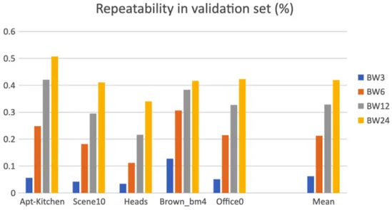
5.1.2 Bandwidth selection . . . 54

5.1.3 Generalization and robustness . . . 55

5.1.4 Overall results . . . 58

5.1.5 Result analysis . . . 58

5.2 StanfordViews . . . 66

5.2.1 Choice of support radius . . . 67

5.2.2 Full-fledged adaptation. . . 68 5.2.3 Overall results . . . 69 5.2.4 Result analysis . . . 70 5.3 ETH . . . 73 5.3.1 Overall results . . . 73 5.3.2 Result analysis . . . 75 6 Conclusions and future developments 77

List of Figures

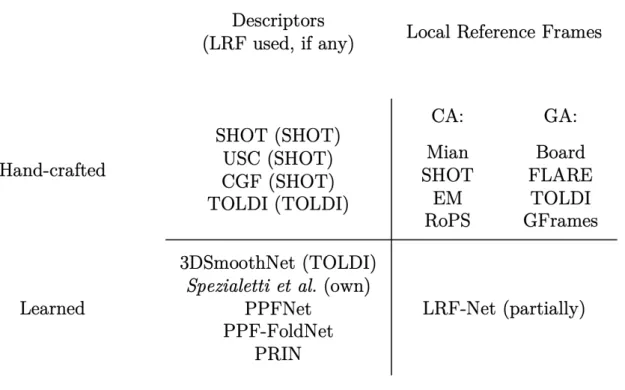
2.1 Categorization of Local Reference Frames and Descriptors. . . 18

3.1 Visualization of 2D discrete correlation. . . 21

4.1 Graphical representation of our network. . . 32

4.2 Example point cloud right after loading. . . 34

4.3 Example cloud after subsampling. . . 34

4.4 Example cloud with highlighted keypoints . . . 35

4.5 Local support of an example keypoint. . . 36

4.6 Local support of an example keypoint after random sampling. . . . 36

4.7 Graphical representation of the spherical voxelization operation. . . 37

4.8 2D graph of the employed piecewise Parzen function. . . 40

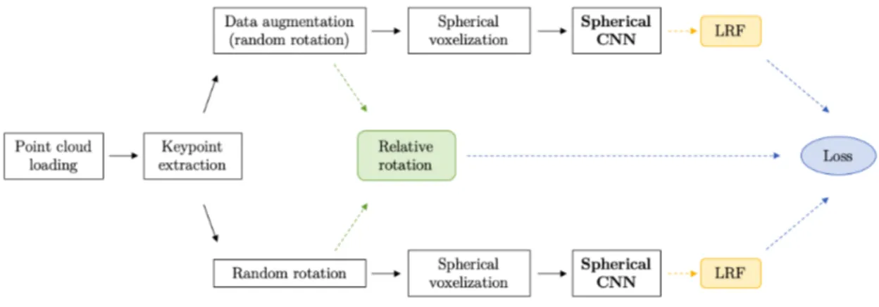
4.9 Unsupervised learning flow chart. . . 41

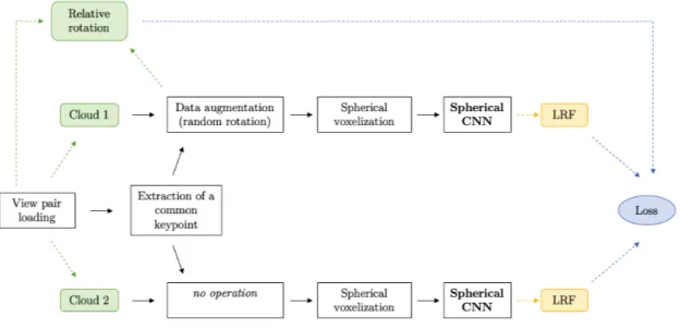
4.10 Weakly supervised learning flow chart. . . 43

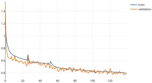
5.1 (3DMatch) Theta loss during a typical training. . . 51

5.2 (3DMatch) Repeatability during a typical training. . . 51

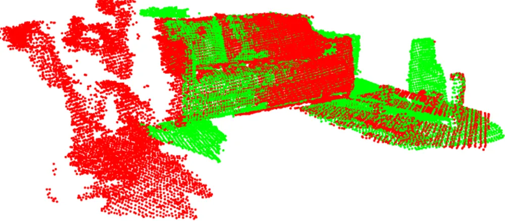
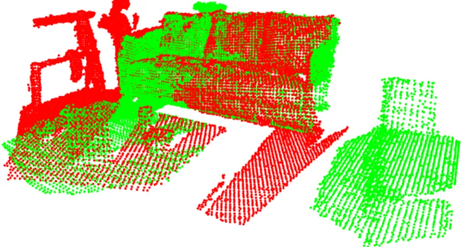
5.3 (3DMatch) Overlap of 2 different views of the same scene. . . 52

5.4 (3DMatch) Overlap of 2 different views of the same scene, rotated. . 53

5.5 (3DMatch) Repeatability during typical trainings. . . 53

5.6 (3DMatch) Benchmark repeatability chart for networks with differ-ent bandwidths (validation set). . . 54

5.7 (3DMatch) Benchmark repeatability chart on the validation set for networks trained with different training sets. . . 55

5.8 (3DMatch) Benchmark repeatability chart on the test set and on a randomly rotated version of it. . . 56

5.9 (3DMatch) Benchmark repeatability chart on the test set comparing presence and absence of sampling operations. . . 57

5.10 (3DMatch) Benchmark repeatability chart on the test set comparing the network to FLARE and SHOT. . . 59

4 LIST OF FIGURES 5.11 (3DMatch) Theta histogram of the validation set with synthetic

rotations, obtained while training an unsupervised network. . . 60 5.12 (3DMatch) Theta histograms of the test scene Home1 with

real-world rotations. . . 60 5.13 (3DMatch) Theta histogram of the network on the validation scene

Apt-Kitchen with real-world rotations. . . 61 5.14 (3DMatch) Visualization with Rodrigues’ vectors of the output layer

of the network. . . 62 5.15 (3DMatch) Alternative visualization with Rodrigues’ vectors of the

output layer of the network. . . 63 5.16 (3DMatch) Scatter plots of the benchmark performances of the

net-work on the validation set. . . 64 5.17 (3DMatch) Scatter plots of the benchmark performances of the

net-work on the test set. . . 65 5.18 (3DMatch) Scatter plots of the benchmark performances of FLARE

on the validation set. . . 65 5.19 (3DMatch) Scatter plots of the benchmark performances of FLARE

on the test set. . . 65 5.20 (StanfordViews) Objects of the StanfordViews dataset. . . 66 5.21 (StanfordViews) Benchmark repeatability chart comparing different

support radii. . . 67 5.22 (StanfordViews) Benchmark repeatability chart comparing different

training methods. . . 68 5.23 (StanfordViews) Benchmark repeatability chart comparing the

net-work to FLARE. . . 70 5.24 (StanfordViews) Theta histograms of the network. . . 71 5.25 (StanfordViews) Theta histograms of FLARE on Armadillo. . . 71 5.26 (StanfordViews) Scatter plots of the benchmark performances of the

network. . . 72 5.27 (StanfordViews) Scatter plots of the benchmark performances of

FLARE on meshes. . . 72 5.28 (StanfordViews) Scatter plots of the benchmark performances of

FLARE on point clouds. . . 72 5.29 (ETH) A view of Gazebo summer. . . 73 5.30 (ETH) Benchmark repeatability chart comparing the network, with

different training methods, to FLARE. . . 74 5.31 (ETH) Theta histograms on Gazebo Winter. . . 75 5.32 (ETH) Scatter plots of the benchmark performances of the network. 76 5.33 (ETH) Scatter plots of the benchmark performances of FLARE. . . 76

List of Tables

5.1 (3DMatch) Benchmark repeatability on the validation set for net-works with different bandwidths. . . 54 5.2 (3DMatch) Benchmark repeatability on the validation set for

net-works trained with different training sets. . . 55 5.3 (3DMatch) Benchmark repeatability on the test set and on a

ran-domly rotated version of it. . . 56 5.4 (3DMatch) Benchmark repeatability on the test set comparing

pres-ence and abspres-ence of sampling operations. . . 57 5.5 (3DMatch) Benchmark repeatability on the test set, comparing the

network to FLARE and SHOT. . . 58 5.6 (StanfordViews) Benchmark repeatability of networks with different

support radii. . . 67 5.7 (StanfordViews) Benchmark repeatability of different training

meth-ods. . . 68 5.8 (StanfordViews) Benchmark repeatability of the network compared

FLARE. . . 69 5.9 (ETH) Benchmark repeatability of the network, with different

train-ing methods, compared to FLARE. . . 74

Chapter 1

Introduction

Computer Vision is a highly interdisciplinary scientific field that aims to pro-vide computers with human-like or superhuman abilities in terms of vision-related tasks, such as object recognition, pose estimation, video tracking, 3D scene recon-struction, augmented reality and many more. It involves mathematics, computer science and artificial intelligence, allowing computers to carry out countless in-dustrial activities (e.g. quality control, defect detection), surveillance duties and consumer-related tasks (e.g. face recognition and visual search), eventually en-abling futuristic applications such as augmented reality and autonomous vehicles. Computer Vision processes images and videos, both 2D and 3D, provided by cam-eras, scanners and depth sensors.

In the context of this work, we will be dealing with 3D data, namely with point clouds: sets of points in the 3D space, generated by scanners and depth cameras. One of the most crucial and researched on problems in 3D Computer Vision is surface matching, i.e. the process of finding similarities between surfaces [29] [15], in order to tell if a surface matches another and, if so, how to align them. Surface matching has applications in a wide variety of fields, such as robotics, automation, biometric systems, 3D scene reconstruction, search in 3D object databases [29], augmented reality, obstacle avoidance and path planning for autonomous vehicles, and has become increasingly relevant due to the availability of off-the-shelf depth sensors such as Microsoft Kinect and Intel RealSense [18]. It also represents the foundation of two very important tasks [22]: surface registration, which is the process of aligning different 3D fragments into a single common coordinate system [27], and 3D object recognition.

In the past, surface matching was handled with global approaches, that suffered from clutter and occlusion problems. Following the trend of 2D Computer Vision, in the last two decades the paradigm has undergone a shift towards local methods, that are able to more effectively withstand such nuisances [22] [29]. A local ap-proach means finding interesting points (called keypoints) on the 3D surface, and

8 CHAPTER 1. INTRODUCTION considering only a limited neighborhood (hereinafter support ) of such points for the computation of compact representations (named descriptors) of such neighbor-hoods. These compact descriptors should be at the same time highly distinctive and robust, in order for corresponding points of two views of the same surface to be successfully matched together. If enough descriptors are matched between a model and a target point cloud, the model object could be present in the target cloud (object recognition); moreover, if enough descriptors are matched, they al-low for the estimation of rigid body transformations, that are the key to surface registration [22].

In order to have such results, the descriptors should be informative enough to avoid false matches as much as possible, while still being robust enough to be matched across point clouds with very different orientations, and withstanding nuisances such as noise, point density variations, clutter and occlusion. The property of being invariant to 3D rigid body transformations is called rotation invariance, meaning that a descriptor should encode information about the shape and not about the pose, and it is a key property for descriptors to carry out their work. In order to achieve it, some authors sacrifice part of the informativeness, some others try to develop a process that is inherently rotation invariant, while a third group relies on the definition of local systems of Cartesian coordinates, called Local Reference Frames (LRFs), which provide a canonical orientation for every local support. The last approach is highly researched on, and aims to create an invariant descriptor by coupling an informative description of the support with a way to orientate the points under consideration.

1.1

Objectives

In the past, a lot of effort has been put into defining high-performing handcrafted Local Reference Frames and descriptors. Recently, following their success in ad-vancing the state of the art for other Computer Vision tasks, there is an increasing interest into employing Artificial Neural Networks to achieve better performances also in surface matching. While interesting results with learned descriptors have already been published, there is still quite little going on about learned LRFs: there exist plenty of methods to compute them but they are all based on hand-crafted algorithms, with the only exception of a recent proposal that deploys neural networks. Yet, it feeds them with manually engineered features, and therefore it does not fully benefit from the modern end-to-end learning strategies. Learned descriptors have allowed for advancements in matching precision and recall, and a successful end-to-end learned solution has been proposed for the first time last year by the team of CV Lab (University of Bologna) [26], showing better results than methods that feed manually engineered features to a network. Thus, the

1.2. THESIS OUTLINE 9 objective of this thesis is to develop an end-to-end learned LRF for point clouds, leveraging the architecture described in [26] and [35], and assess its performances compared to the current state of the art. The final objective is to do so with unsupervised learning methods, because they do not require ground-truth data, which is cumbersome to obtain for surface matching, but partial results deriving from supervised methods will be presented as well.

1.2

Thesis outline

The first part of this thesis (Chapter 2) will briefly review the most important existing works on LRFs for point clouds, showing their working princples and the absence of fully learned LRFs. Hints on local descriptors will be given as well. The second part (Chapter 3) will present a mathematical explanation of the con-cepts that underlie the proposed method, followed, in Chapter 4, by a description of such method, of the employed neural network and of the training and bench-marking processes.

The last part (Chapter 5) will describe the datasets used for the experimental validation, and show the results.

Chapter 2

Related works

A wide variety of different LRFs have been proposed in the literature. This chap-ter will list the most influential and performant ones, describing their working principles. The last section will also mention some local descriptors and the use they make of LRFs, showing the lack of a fully learned LRF.

2.1

Local Reference Frames

As stated in [18] and [33], hand-crafted LRF estimation methods can be divided as based upon Covariance Analysis (CA) or Geometric Attributes (GA). The former group includes the LRF used by Mian et al. [19], SHOT [29] [24], EM [20], RoPS [14], along with many others, while the latter group includes PS [3], Board [22], FLARE [21], TOLDI [34] and GFrames [18]. To the best of our knowledge, the only example of a data-driven approach for LRFs is represented by the work of Zhu et al., posted as pre-print on ArXiv in January 2020 [37], that will also be briefly presented in this chapter.

Definition 2.1. (LRF). [18] Given a point cloud P, the LRF of point p ∈ P is defined as

L(p) = {ˆx(p), ˆy(p), ˆz(p)} (2.1) where ˆx(p), ˆy(p), ˆz(p) are the orthogonal axes of the coordinate system, satisfying the right-hand rule ˆy = ˆz ∧ ˆx.1

Thus, defining an LRF means defining a way to compute each one of its axes. Moreover, for the following sections:

• let p ∈ P be the point for which we want to compute the LRF,

1_{Bold means vector notation (column matrices) and the circumflex means unit vector.}

Brack-ets with the indication of the point can be omitted if the point is not ambiguous.

12 CHAPTER 2. RELATED WORKS • let NR(p) be the support of radius R around p,

• let pi ∈ NR(p) for i = 0, . . . , k,

• let ˆn(p) be the normal to the surface at point p.

2.1.1

CA-based methods

All the methods belonging to this category share the need of a covariance matrix of the points in the local support, and they differ from each other in the way they use this information to compute the axes.

Mian [19]. It has been proposed in 2010, and basically employs Principal Com-ponent Analysis in order to determine 3 orthogonal unit vectors. In fact, given a point p and its local support, it computes the normalized eigenvectors of the following covariance matrix:

Σbp = 1 k k X i=0 (pi− bp)(pi− bp)T (2.2)

with bp being the the barycenter of the points in NR(p):

bp = 1 k k X i=0 pi (2.3)

The problem with this method is that eigenvectors define the direction only, whereas their sign is ambiguous. Disambiguation happens for the z axis only, that is chosen so as to have a positive product with the normal ˆn(p), but am-biguity remains for the other axes, implying that this method potentially defines multiple LRFs for a single point, a fact that greatly increases the time requirements to match points in different point clouds [21] [33].

SHOT [29] [24] It has also been proposed in 2010. It is the first CA method that removes the ambiguities in the axes [29] [33], and it has become one of the most popular LRFs in the literature. It computes a slightly different, weighted covariance matrix, that proved to be more robust against clutter:

Σpw = 1 Pk i=0(R − di) k X i=0 (R − di)(pi− p)(pi− p)T (2.4)

with the L2 distance di = kpi− pk₂ < R. Notice that the barycenter has been

2.1. LOCAL REFERENCE FRAMES 13 The eigenvectors resulting from the covariance matrix are assigned in decreasing eigenvalue order to x+, y+, z+, while their opposites are referred to as x−, y−, z− Disambiguation is carried out on the x and z axes as follows:

S_x+ := {i : di < R ∧ (pi− p) · x+ ≥ 0} S_x− := {i : di < R ∧ (pi− p) · x− > 0} ˆ x = ( x+ _{if |S}+ x| ≥ |S − x| x− otherwise (2.5)

and analogously for z, meaning that the sign of an axis has to be coherent with the majority of the points in the support. For the remaining axis, ˆy = ˆz ∧ ˆx. This method provides a good balance in terms of efficiency, repeatability and robustness to clutter and occlusion. However, its feature matching performance is not always paralleled by its repeatability [33].

2.1.2

GA-based methods

These methods typically compute their axes successively, possibly in different ways, leveraging geometric attributes such as normals and signed distances [33].

Board [22]. Proposed in 2011, it is the result of an extensive analysis of existing proposals. It is based on the definition of two different supports: NRz(p) and

NRx(p), typically set to have Rz small and Rx > Rz.

Firstly, it fits a plane on the points of NRz(p) and takes its normal (z

+_/z−_{). It}

then computes the average normal ˜n across support points, and chooses between z+ and z− so to have a positive inner product with ˜n.

Secondly, for each point p_i ∈ NRx(p) it computes the cosine of the angle between

ˆ

z and the average normal at that point, named ˜n(p_i). The point p_min with the lowest cosine (highest angle) is selected, and the vector from p to p_min is projected onto the tangent plane on p and normalized, to become the x axis. Since p_min almost always lies in the outer regions of the support, the computation is sped up by considering only the support points with distance from p greater than a defined threshold, usually 0.85 · Rx.

As usual, the y axis is computed by cross-product.

Board also takes into account the possibility to have missing regions, defining a heuristic procedure to estimate if p_min lies in the missing region or not.

FLARE [21]. Proposed in 2012, it is a modified version of Board, by the same authors. It computes the z axis as in Board, but for the x axis it uses the signed

14 CHAPTER 2. RELATED WORKS distance instead of the cosine with the normal.

The signed distance of a point p_i is defined as:

dSD(pi) = ppi · ˆz (2.6)

with pp_i being the vector going from p to p_i. The algorithm selects the point with the largest signed distance, which is the point whose component parallel to the z axis is the largest, meaning the most distant point from the tangent plane at point p. As before, the projection of this point to the tangent plane is normalized and taken as the x axis.

FLARE has proven to be more repeatable than Board, but they both have similar problems with noise and outliers [33].

TOLDI [34]. Proposed in 2016, it computes the z axis in a very similar fashion to CA methods, as it computes the covariance matrix (using the barycenter) and considers as z+ the unit eigenvector with the smallest eigenvalue. The first differ-ence is that this covariance is computed on NR

3(p) instead of NR(p). The other

difference is in the disambiguation of the sign, that follows the rule: ˆ z = ( z+ _{if z}+_·P pi∈NR(p)pip ≥ 0 −z+ _otherwise (2.7)

The x axis will lie in the tangent plane of p with respect to the normal ˆz, but finding an orientation for such plane is more difficult than finding ˆz.

The first step is the computation of the projections of the support points on the plane. For each p_i ∈ NR(p),

vi = ppi− (ppi· ˆz(p)) · ˆz(p) (2.8)

The x axis is then computed as a weighted sum: ˆ x = 1 k P i=0 wi1wi2vi 2 k X i=0 wi1wi2vi (2.9)

In this sum, wi1 is related to the distance of the point and is designed to improve

robustness to clutter, occlusion and incomplete border regions, while wi2 is set

to make the points with larger projection distance contribute more to the x axis, since such distance feature is a distinctive cue and can provide high repeatability on flat regions. They are defined as follows:

wi1= (R − kp − pik2)

2.1. LOCAL REFERENCE FRAMES 15

wi2= (ppi· ˆz(p))

2 _(2.11)

As usual, the y axis is computed by cross product.

TOLDI can produce great performances, but it has been shown to be quite sensitive to keypoint localization error [33].

GFrames [18]. It has been proposed in 2019 by a team of researchers from different institutions, including the University of Bologna.

It assumes that the point cloud (or the mesh) is a sampling of a 2D Riemannian manifold embedded in the R3 _{space. Since the method needs the areas of the}

mesh triangles, it works straight away with meshes, while for point clouds it uses a procedure that locally computes estimates of triangles.

The z axis is defined as the normal on the point, ˆn(p), while for the x axis it computes the following formula:

x(p) := _P 1

tj∈NR(p)A(tj)

X

tj∈NR(p)

A(tj)∇f (tj) (2.12)

with tj a mesh triangle, NR(p) the set of triangles within distance R from p, A(tj)

the area of the tj triangle and f a user-defined scalar function.

The actual ˆx(p) is computed by projecting the result of equation 2.12 on the plane defined by ˆn(p) and normalizing the projection to have a unit vector. The remaining axis is the usual cross product.

In [18], different f functions are tested, such as the mean curvature, the Gaussian curvature, the sum of total Euclidean distances, and the function of FLARE itself (average of the signed distances from tangent plane), showing great robustness and repeatability. GFrames is also particularly suited for non-rigid transformations, thanks to its flexibility.

2.1.3

Data-driven methods

As previously stated, to the best of our knowledge there exist a single public data-driven method applied to learning a Local Reference Frame for point clouds, named LRF-Net. Nevertheless, the aforementioned approach does not rely on feeding the network with the raw information from the point cloud: it feeds hand-crafted features computed on the point cloud, instead. Thus, there are currently no public proposals of end-to-end learning applied to Local Reference Frames. LRF-Net [37]. Proposed at the beginning of 2020, it is the first data-driven approach for LRFs.

16 CHAPTER 2. RELATED WORKS In spite of being data-driven, it still relies on a traditional approach to compute the z axis, that is in fact set to be equal to the normal ˆn(p) of the keypoint p. The x axis, instead, is computed by the following formula:

ˆ x(p) = 1 k P i=0 wivi 2 k X i=0 wivi (2.13)

with vi defined as in equation 2.8 to be the projection of ppi on the tangent plane.

The weights wi are computed by an Artificial Neural Network, consisting of 8 fully

connected layers with batch normalization and ReLUs after each layer.

The network has a 2D input layer and a 1D output layer, with the inputs being ai

dist and aiangle for point pi ∈ NR(p), defined as follows:

(

ai_dist = kpp_ik₂/R

ai_angle = cos(ˆz(p), pp_i) (2.14) Basically, the first one is the fraction of the distance of the i-th point with respect to the maximum distance of the support, and the second one is the cosine between the normal on the keypoint and the vector from the keypoint to the i-th point. The network computes each weight separately.

As stated in [37], these features are complementary to each other, providing in-formation about distance and angle for each point in the support, and are also invariant, provided that z is repeatable. This is crucial for the network to produce an invariant output, which is used to compute a linear combination of the vis,

equivariant by definition, thus providing an x axis that rotates along with the point cloud as long as the z axis is repeatable.

The network is trained in a weakly supervised, Siamese, way (more on this in Chapter 4), loading corresponding pairs of keypoints from point clouds recorded from different viewpoints, rotating each keypoint with its support according to the LRF computed as defined above, and minimizing the Chamfer Distance [1] between the two rotated local supports.

2.2

Local descriptors

Since local descriptors, which are compact representations of the neighborhood of a point, are out of the scope of this work, this section will not go into detail about how they are computed.

It’s worth noting that most of the Local Reference Frames deliver their best performances under very specific circumstances and/or particular applications [33],

2.2. LOCAL DESCRIPTORS 17 or when coupled with their respective descriptor: in fact, part of the papers that define a Local Reference Frame do so in order to support the definition of a custom local descriptor. Mian, SHOT and TOLDI, for example, define both a LRF and a descriptor, whereas Board, FLARE and GFrames do not.

Other notable descriptors, defined separately from LRFs, are USC (Unique Shape Context, 2010) [28], CGF (Compact Geometric Features, 2017) [16] and 3DSmooth-Net (2018) [12]. Both the first two use SHOT, and are hand-crafted, while the last one uses a slightly modified version of TOLDI and is a learned descriptor. Other learned descriptors, that do not rely on LRFs, are PFFNet [11], PPF-FoldNet [10] and PRIN [35], all from 2018.

An interesting example of a non-invariant learned descriptor that does not rely on hand-crafted features and that also defines its own LRF, is described in [26] by Spezialetti et al.2_{. By taking advantage of spherical convolutions, their}

net-work processes a spherical signal (directly computed from the point cloud), and computes a 512-dimensional codeword that is used as an equivariant descriptor. Being equivariant, it is theoretically possible to compute the rotation between two descriptors (or intermediate feature maps) by computing the arg max of the correlation between the two. However, this is practically impossible to do when matching descriptors, since doing that for every possible pair of descriptors re-quires a tremendous amount of computing time. Because of this reason, they decided to choose a heuristic on the descriptor, for example the highest value. If the descriptor is perfectly equivariant, this maximum will be present in different bins in the descriptors of corresponding keypoints in two rotated point clouds. Thanks to the structure of the network and to the mathematical properties of spherical convolutions, it is possible to analyze the position of these maxima and infer the rotation operation that aligns them. As a consequence, the position of the maximum can be used to define a Local Reference Frame in such a way that the descriptor, orientated according to the LRF, becomes invariant to input rota-tions. While theoretically interesting, the highest value alone is not robust enough to reach good results in practice, and a different heuristic has been used, involving the computation of the density of the top k values.

Such learned descriptor, coupled with the proposed LRF, achieves great perfor-mances, but they can be further improved by using FLARE as the LRF, as shown in [26]. Due to the promising mathematical properties of the network, though, it seems to be possible to use the proposed framework to specifically learn a Local Reference Frame, and this is where this thesis lays its foundations.

To sum up, here is a table (figure 2.1) that categorizes all the cited methods. Hand-crafted LRFs are divided as in [33]; each descriptor is followed by the LRF it makes use of, except for PPF-based descriptors and PRIN; lastly, there is an

18 CHAPTER 2. RELATED WORKS evident gap in learned Local Reference Frames, as the present method doesn’t use end-to-end learning and is employed for just one out the three axes of the coordinate system.

As of now, FLARE, TOLDI and GFrames are considered state-of-the-art meth-ods, with FLARE being selected for direct comparisons with the method developed in the next chapters.

Chapter 3

Theoretical background

The aim of this chapter is to provide all the required concepts to understand Spherical Convolutional Neural Networks and the architecture proposed in Chapter 4.

Most of this chapter is based on the renowned book “Deep Learning”, by Good-fellow, Bengio and Courville [13] and on the work of Cohen, Geiger, Koehler and Welling about group equivariant neural networks and Spherical CNNs [4] [5] [6], although with changes in notation. For this reason, citations to the aforementioned works will be avoided, whereas different sources will be cited when used.

The chapter will first present a brief recap on standard convolution, correlation and CNNs: their short description is mainly provided to set the notation for the equations, and to offer a parallel presentation of them and the core theoretical part, Spherical CNNs.

The chapter will then describe the possible ways to represent rotations in 3D space, followed by the definition of a quality measure for Local Reference Frames, that will be used to assess the performance of the proposed method.

3.1

Standard CNNs

Definition 3.1. (1D Convolution). For continuous real-valued scalar signals f, g : R −→ R, convolution is defined as:

h(t) = [f ∗ g](t) = Z +∞

−∞

f (τ )g(t − τ )dτ (3.1) while for discrete signals it is sufficient to substitute the integral with a sum.

The result of convolution is not a number, it is a function h : R −→ R whose domain is the same of f and g. The output of h for a certain input t is the integral

20 CHAPTER 3. THEORETICAL BACKGROUND (or sum) of the product between f and g, with the latter being flipped around the origin and translated by t. As a consequence, it is possible to visualize the h function as a 1D signal, with each value computed as stated above.

Convolution is a commutative operation.

Definition 3.2. (1D Correlation). Similarly, correlation is defined as: i(t) = [f ? g](t) =

Z +∞

−∞

f (τ )g(τ + t)dτ (3.2) with i : R −→ R. Again with a sum in case of discrete signals.

As a difference, correlation does not flip the g function, and is not commutative. These two operations are strongly connected to each other, and are often used interchangeably if the g function is symmetric. In fact, it is possible to compute convolution using correlation by simply flipping the second function and inverting the order (so that the first function gets translated instead of the second), and vice-versa, with flipping being unnecessary if g is symmetric.

All of this can be straightforwardly generalized to signals on the plane, and thus it can be applied to images, that are in fact 2D discrete signals. All the following formulas can be expressed with summations instead of integrals to cope with discrete signals.

Definition 3.3. (2D Convolution). Let f, g : R2 _{−→ R, the 2D Convolution is}

defined as: h(x, y) = [f ∗ g](x, y) = Z +∞ −∞ Z +∞ −∞ f (α, β)g(x − α, y − β)dαdβ (3.3) with x, y ∈ R and h : R2 _{−→ R.}

Definition 3.4. (2D Correlation). Similarly, the 2D Correlation is defined as: i(x, y) = [f ? g](x, y) = Z +∞ −∞ Z +∞ −∞ f (α, β)g(α + x, β + y)dαdβ (3.4) with i : R2 _{−→ R.}

As for the 1D case, computing a convolution between two signals means over-lapping (by multiplication) the input functions and computing their sum or inte-gral, with the second function being flipped around the origin and translated by a quantity specified by the input of the convolution function.

If we say that f is an image and g is a kernel (or filter), i.e. two real-valued discrete functions on the plane, the output of a correlation/convolution can be

3.1. STANDARD CNNS 21

Figure 3.1: Visualization of 2D discrete correlation, image from [13]. Notice that in case of a finite domain the output dimensions are smaller than the input, because placing the kernel out of the image is a (usually) not allowed operation.

easily visualized as in figure 3.1. It is an image itself, whose pixels are computed by multiplying the original image and an accordingly shifted kernel. The actual operation in this image is a correlation between the kernel and the image (not commutative), with convolution being analogous (with a flipped kernel).

Convolutional Neural Networks (CNNs) take their origin from the aforemen-tioned operations of convolution and correlation and, in spite of the name, they usually employ correlation as the layer operation, while convolution arises dur-ing backpropagation. In fact, the key difference between a MultiLayer Perceptron (MLP) and a CNN is that the former computes a matrix multiplication between inputs and weights as the layer operation, while the latter uses correlation between the input to the layer and a set of filters, that are simply small kernels like in figure 3.1.

In the previously defined correlation, an input of (x, y) means translating the filter by (−x, −y), thus practically flipping the output map with respect to the origin. In order to have a direct correspondence between a point of the output and a point

22 CHAPTER 3. THEORETICAL BACKGROUND of the input, as in figure 3.1, the usual operation that happens in CNNs is a variant of correlation that corresponds to a correlation with commuted input functions. Definition 3.5. (CNN Layer Operation). Consider a CNN with n layers. The input of each layer l is a feature map f : Z2 _{−→ R}Kl

, the number of output channels for layer l is Kl+1_{, and the K}l+1 _{filters for layer l are ψ}i _{: Z}2 _{−→ R}Kl

for i = 1, . . . , Kl+1. The output of layer l is defined as:

[f ? ψi](x, y) = +∞ X α=−∞ +∞ X β=−∞ Kl X k=1 fk(α, β)ψki(α − x, β − y) (3.5)

with i = 1, . . . , Kl+1_{. Feature maps and filters are considered to be defined}

every-where in Z2 _{and 0-valued in out-of-map domain points.}

Interestingly, each filter has as many channels as the input, and each correlation produces a real-valued output. Thus, each correlation is computed on all the input channels, which are eventually summed together to produce the output.

The parameters learned by a CNN (i.e. the weights) are the values of the filters. This approach has 3 main advantages:

• It greatly reduces the number of parameters, because filters are chosen to be much smaller than the input images;

• It allows for weight sharing, because each pixel of the output is computed with the same weights but with a different input (portion of the input image); • It is equivariant to translations, meaning that if a certain input produces a certain output when correlated with a filter, then the same input in a different portion of the image will produce the same output but in a correspondingly different portion of the output feature map.

The last property is the most interesting for the purposes of this work, so here is a more precise definition of it.

Definition 3.6. (Equivariance). [31] [2] Let G be a set of transformations. Consider a function Φ : X −→ Y that maps inputs x ∈ X to outputs y ∈ Y. A transformation g ∈ G can be applied to any x ∈ X by means of the operator TX

g : X −→ X , such that x is transformed to T X

g [x], and analogously for y ∈ Y

transformed to T_gY[y]. Φ is said to be equivariant to G if:

3.1. STANDARD CNNS 23 The operators T_gX[x] and T_gY[y] are basically the application of the same trans-formation g to elements from different domains, and are related by the equation above. Invariance, instead, is a particular case of equivariance in which the op-erator T_gY[y] is the identity transformation, meaning that the result of Φ doesn’t change with a transformation of the input.

It is possible to apply this definition of equivariance to the operation defined in equation 3.5, and thus to Convolutional Neural Networks. In fact, if we consider Φ as the layer operation, x ∈ X as a point of the input image, y ∈ Y as a point of the output, and G as the set of 2D translations (with T_gX[x] = T_gY[y] as the application of such translations), it is trivial to see that CNNs are translation-equivariant. By defining the operator Lt,s to take a 2D function and translate it by (t, s) as

[Lt,sf ](x, y) = f (x − t, y − s) (3.7)

translation-equivariance can be proved as follows, by substituting α with α + t and β with β + s (channels are dropped to slim down notation):

[Lt,sf ? ψ](x, y) = +∞ X α=−∞ +∞ X β=−∞ f (α − t, β − s)ψ(α − x, β − y) = +∞ X α=−∞ +∞ X β=−∞ f (α, β)ψ(α + t − x, β + s − y) = +∞ X α=−∞ +∞ X β=−∞ f (α, β)ψ(α − (x − t), β − (y − s)) = [f ? ψ](x − t, y − s) = [Lt,s[f ? ψ]](x, y) (3.8)

It is also worth noting that in a convolution or correlation, let’s say for con-tinuous 2D signals, the domain of the input functions f and g is the plane R2_,

whereas the domain of the output function (so the domain of the convolution or correlation itself) is the subgroup of 2D translations (because computing the op-eration for (x, y) means translating the g function by (x, y)), which is isomorphic to the plane R2_{. This is a subtle difference, because such subgroup acts on itself,}

but it will be useful for the next section as this is not always the case.

Going back to the aim of this thesis, which is finding a Local Reference Frame, it is important to notice what follows: given a keypoint with its local support, a LRF will set 3 axes, defining an orientation for such keypoint1. If the same keypoint is rotated and then a LRF is computed, we expect the LRF to produce

24 CHAPTER 3. THEORETICAL BACKGROUND the same axes as before with respect to the shape of the support, meaning that the two keypoints can be perfectly aligned. In other words, this means that the LRF should rotate in the 3D space along with the input, and thus that the LRF should possess the 3D rotation-equivariance property. How to achieve it?

3.2

Spherical CNNs

Cohen et al. [5] [6] have shown that it is possible to achieve equivariance to rotations in space by using spherical signals and spherical convolutions. Their theory has been developed for spherical images, i.e. images that are defined on a sphere instead of a plane, because the usual way to handle these images was to use standard CNNs with multiple planar projections, a sub-optimal approach due to planar projections producing distortion. By using their method, it is possible to define a natural convolution on the sphere itself.

The input format for this work, though, is not a spherical signal, it is a point cloud. However, there are multiple ways to transform point clouds into spherical signals: ray casting [6] and spherical voxelization [35] are two examples, with the latter being deployed in this context and described in the next chapter. Thus, we can consider to be able to use spherical signals and continue with the dissertation. Definition 3.7. (S2_{). The unit sphere S}2 _{is defined as the set of points x ∈ R}3

with norm 1. It’s a 2-dimensional manifold that can be parametrized with spherical coordinates α ∈ [0, 2π] and β ∈ [0, π].

Definition 3.8. (Spherical Signal). A spherical signal is a vector-valued func-tion f : S2 −_{→ R}K_{, with K as the number of channels.}

Definition 3.9. (SO(3)). 3D linear transformations can be represented by 3x3 matrices, and the set of 3x3 matrices with orthonormal columns, along with matrix multiplication, forms the Orthogonal group O(3). This group is made of two connected components, one with determinant 1 and the other one with determinant -1. The first component also contains the identity matrix, and thus is a subgroup containing all the rotations in 3D space. This subgroup is called SO(3), the Special Orthogonal group for 3 dimensions, also known as rotation group.

SO(3) is a 3-dimensional manifold, and can be parametrized in many different ways. The following formulas will consider a parametrization wih ZYZ-Euler an-gles α ∈ [0, 2π], β ∈ [0, π] and γ ∈ [0, 2π]. Moreover, in order to apply rotations to spherical signals by matrix multiplication, points on the sphere S2 can be consid-ered as 3D unit vectors. Rotations and their representations are further described in section 3.3.

3.2. SPHERICAL CNNS 25 Definition 3.10. (Rotation of Spherical Signals). Given a spherical signal f : S2 −_{→ R}K _{and a rotation R ∈ SO(3), the rotation operator L}

R rotates the

signal as:

[LRf ](x) = f (R−1x) (3.9)

with x ∈ S2_{. By rotating the input by the inverse of R, it effectively rotates the}

signal by R. Notice that LRR0 = L_RL_R0.

Definition 3.11. (Inner Product). Spherical signals constitute a vector space. Thus, given two K-valued spherical signals f, ψ : S2 _{−→ R}K_{, their inner product}

can be defined as:

hψ, f i = Z S2 K X k=1 ψk(x)fk(x)dx (3.10)

with dx as the standard rotation invariant integration measure on the sphere, dx = dα sin(β)dβ/4π in spherical coordinates α and β.

An invariant measure means that the integral doesn’t change with rotations, and thus that the inner product between two functions doesn’t change if they are rotated by the same rotation R:

hLRψ, f i = Z S2 K X k=1 ψk(R−1x)fk(x)dx = Z S2 K X k=1 ψk(x)fk(Rx)dx = hψ, LR−1f i (3.11)

With the concepts defined above, it is possible to proceed to define a correlation for spherical signals, that will constitute the fundamental block of Spherical CNNs. Definition 3.12. (Spherical Correlation). Let f, ψ : S2 −_{→ R}K_{, their spherical}

correlation is: [ψ ? f ](R) = hLRψ, f i = Z S2 K X k=1 ψk(R−1x)fk(x)dx (3.12)

Let’s now compare this function to equation 3.5, that is the standard CNN correlation. They look very similar to each other, with the spherical correlation that looks to be its direct generalization to spherical signals. But here the subtle difference about the domain of the resulting function arises. In fact, while standard correlation is defined on the subgroup of 2D rotations, that is isomorphic to R2

26 CHAPTER 3. THEORETICAL BACKGROUND domain of a spherical correlation is the set of 3D rotations: SO(3). It is possible to visualize this by thinking of two spheres, that can be multiplied to each other after being rotated in all 3 dimensions. In the 2D domain it would be equivalent to being able not only to translate the maps, but also to rotate them around one of their points.

By using this spherical correlation as the layer operation for Spherical CNNs, we immediately face a change in the domain of the signals. Indeed, despite the fact that the input to the first layer is an S2 signal, and so are its filters, the output of such layer will be a signal defined on SO(3), with as many channels as the number of filters. We should then repeat this process for SO(3) signals, as follows.

Definition 3.13. (Rotation of SO(3) Signals). Given an SO(3) signal f : SO(3) −_{→ R}K and a rotation R ∈ SO(3), the rotation operator LR can be

straight-forwardly generalized to rotate the SO(3) signal as:

[LRf ](Q) = f (R−1Q) (3.13)

with Q ∈ SO(3). Notice that, in this case, both R and Q belong to SO(3).

Definition 3.14. (SO(3) Correlation). Let f, ψ : SO(3) −_{→ R}K_{, their spherical}

correlation is: [ψ ? f ](R) = hLRψ, f i = Z SO(3) K X k=1 ψk(R−1Q)fk(Q)dQ (3.14)

with dQ as the invariant measure on SO(3). If we parametrize it with the afore-mentioned ZYZ-Euler angles, it is dQ = dα sin(β)βdγ/(8π2_).

This time, the domain of SO(3) correlation is SO(3) itself, which is a group. At this point, we have both layer operations required to build a Spherical CNN, whose peculiar characteristic is the equivariance to rotations, and is thus suitable to our needs. By recalling the definition of equivariance (definition 3.6), and considering Φ as the correlation, x as point on the sphere or on SO(3), y as a point on SO(3), G as SO(3) itself, and Tg as LQ, the proof proceeds as follows.

[ψ ? [LQf ]](R) = hLRψ, LQf i (3.15)

Using the invariance property of the inner product (equation 3.11) and the property at the end of definition 3.12, we have:

hLRψ, LQf i = hLQ−1_Rψ, f i (3.16)

By using, respectively, the definition of correlation (3.12 and 3.14) and the defini-tion of rotadefini-tion (3.10 and 3.13), we can end the proof:

3.3. REPRESENTATIONS OF ROTATIONS 27 This proof applies to both spherical and SO(3) correlation.

We have now a complete definition of rotation-equivariant Spherical CNNs, whose first layer computes the spherical correlation and the following layers com-pute the SO(3) correlation. In these peculiar CNNs, the first layer has spherical signals as filters, whereas the other layers have signals on SO(3).

In practice, though, to speed up the computation, layers employing spherical or SO(3) correlation do not directly compute those transformations. Instead, they compute their results using a Generalized Fast Fourier Transform, but this is out of the scope of this work. More on this can be found in [6].

3.3

Representations of rotations

There are many different ways to represent rotations in the 3D space. This section will briefly show the ones used for this work, namely: Euler angles, 3x3 matrices, axis-angle and Rodrigues’ vectors. Quaternions are another very interesting rep-resentation, especially for machine learning purposes, but they will not be covered since they haven’t been used.

Before starting, it’s worth noting that a Local Reference Frame can be identified exactly as the rotation that transforms the original coordinate system of the point cloud into the new coordinate system, or as the inverse of such rotation. So, the following representations also apply to LRFs.

3.3.1

Euler angles

Let us have a coordinate system (or Local Reference Frame, they are synonyms in this context) to be rotated. It is possible to visualize its rotation by duplicating the coordinate system, fixing one copy, and rotating the other. Since rotations in 3D space have 3 degrees of freedom, only 3 parameters are necessary to charac-terize a rotation. If we imagine to rotate the moving copy around the Z axis first, then around the Y axis, and finally around the X axis, the 2D rotation angles around such axes are known as the 3 Euler angles α, β and γ. Consequently, a full rotation will be the composition of such 3 transformations (XYZ).

As previously stated, in this context we will consider the ZYZ-Euler angles, mean-ing that both the first and the last angles will refer to rotations around the Z axis. This does not lower the degrees of freedom as long as the rotation around Y is not null, as will be clearer when dealing with matrices.

28 CHAPTER 3. THEORETICAL BACKGROUND

3.3.2

3x3 matrices

2x2 rotation matrices can be straightforwardly generalized to 3D rotations by combining 2D rotations around different axes. If we take the previously defined XYZ-Euler angles, and by defining Rx(α) as the rotation matrix of α around the

X axis, and analogously for the other axes, a full 3D rotation matrix is:

R = Rx(α)Ry(β)Rz(γ) (3.18) where: Rx(α) =   1 0 0 0 cos α − sin α 0 sin α cos α   (3.19) Ry(β) =   cos β 0 sin β 0 1 0 − sin β 0 cos β   (3.20) Rz(γ) =   cos γ − sin γ 0 sin γ cos γ 0 0 0 1   (3.21)

In case of a ZYZ representation it is easy to see that, as long as the Y rotation is not null (and thus the Ry matrix is not an identity matrix), all the rows and

columns of the resulting rotation R have values that, overall, depend on 3 differ-ent parameters, effectively producing a new coordinate system with 3 degrees of freedom.

The rotation matrix is the most used representation to identify Local Reference Frames throughout this work: if we use the rotation matrix that transforms the original axes into the LRF, then the axes of the LRF are the columns of such matrix; whereas if we use the transposed2, the axes are the rows, and such matrix can be directly applied to points to change their coordinate system into the new one. Definition 2.1 considers the LRF as the former case, thus with axes on columns, whereas the code used for learning and benchmarking will mostly use the latter for practical reasons involving arrays.

3.3.3

Axis-angle representation

Another very intuitive way to refer to a 3D rotation is the axis-angle represen-tation. In fact, defining an axis (a line through the origin) and a rotation angle along that axis is sufficient to completely characterize a rotation in R3. Having a

2_{Rotation matrices are orthogonal and, as such, their inverse equals their transpose: R}−1₌

3.4. LRF QUALITY MEASURE: REPEATABILITY 29 rotation matrix R, the points of the rotation axis stay the same before and after the rotation, and are thus the invariants of the rotation. As a consequence, for such points p we have:

Rp = Ip (3.22)

where I is the 3x3 identity matrix.

By solving the equation above we can find the eigenvectors corresponding to the unitary eigenvalue, and use one of them to refer to the rotation axis.

To find the rotation angle θ, it is possible to use the following formula:

Tr(R) = 1 + 2 cos θ (3.23) where Tr is the trace operation.

3.3.4

Rodrigues’ vector

This representation will be very useful for visualization purposes, because it allows to represent a rotation as a single 3x1 vector, whose elements are called Euler-Rodrigues parameters.

Definition 3.15. (Rodrigues’ vector.) [9] Let ˆu = [ux, uy, uz]T be the 3D

unit vector that represents the rotation axis in the axis-angle representation of rotations, and let θ be the angle. The Rodrigues’ vector b is defined as:

b =   bx by bz  =   uxtan θ₂ uytanθ₂ uztanθ₂  = tan θ 2 · ˆu (3.24) The vector b thus represents the rotation axis, with norm equal to the tangent of half of the rotation angle.

In Chapter 5, this representation will be used to show the output feature maps, but the tangent will be dropped in order to have a better scale for visualization.

3.4

LRF quality measure: repeatability

The last thing we need is a measure of how good a LRF is performing.

In the literature, plenty of different measures have been proposed, mostly in-volving the computation of the distance between the computed LRFs on a keypoint from two different (i.e. rotated) viewpoints. But, as noticed in [22] and [21], the problem with this approach is that it doesn’t take into account the fact that LRFs work only if they are almost perfectly equivariant to rotations of the keypoint, and

30 CHAPTER 3. THEORETICAL BACKGROUND are able to align different views of the same keypoint. If a pair of rotated key-points produces LRFs that do not match, it doesn’t matter if it is by 30 degrees or by 180 degrees (the maximum possible): they are simply not repeatable, and thus they would not work if used for pose estimation or keypoint matching. For this reason, Petrelli and Di Stefano proposed in [21] a new quality measure, called repeatability. In this work, their definition has been extended to include 2 axes of the LRF instead of a single one, because here the normal axis is not computed in a standard way as in methods described in Chapter 2. Computing it also for the third axis is not needed, since it is uniquely identified from the other two.

Definition 3.16. (LRF Repeatability.) Let D be a dataset with M different views {V1, V2, . . . , VM}, and let ph ∈ Vh and pk ∈ Vk (with h, k = 1, . . . , M and

h 6= k) be the same point p in two different views. Suppose to have an algorithm to determine a LRF and let L(ph), L(pk) be the computed LRFs for such point3.

We say that the LRFs for corresponding points ph and pk are repeatable if:

ˆ x(ph) · ˆx(pk) ≥ T h and ˆ x(ph) · ˆx(pk) ≥ T h (3.25) with T h as a user defined threshold, usually set to 0.97 in this context. The dot means scalar product, and thus produces the cosine between the axes, since their norm is unitary.

Intuitively, this means that a LRF is repeatable if, when computed on corre-sponding points, it is able to align their coordinate systems with a minimum cosine of T h for each axis.

The repeatability on a whole scene or dataset is then computed as the percentage of repeatable keypoints over the total number of identified keypoints.

Chapter 4

Architecture and methodologies

This chapter will show how we have employed the previously described rotation-equivariant operations to estimate LRFs. It will illustrate the architecture of the neural network, the process that transforms input data (point clouds) to output data (LRFs), and the methodologies that have been used to train and test the network. In the course of this chapter there will be some numeric values: they refer to figure 4.1 and represent the best hyperparameters we have found for the network. For the purpose of this chapter they are to be taken as examples.

As for project technicalities, the programming language we used is Python (v3.6.8), with PyTorch (v1.0.0) as the framework for neural networks; Spherical CNNs are built using the original implementation of [6], that can be found on GitHub1. Training and testing Spherical CNNs is a very heavy and time-consuming task, so it has been partially sped up by employing GPUs and CUDA. All the trainings and tests have been executed on an Intel i7-4790K with a Gigabyte GeForce GTX 970 G1, or on an Intel i7-8700 with an NVIDIA Titan V (Volta) and an NVIDIA GeForce RTX 2080 Ti.

4.1

Network architecture

The neural network we used is almost entirely made of convolutional layers, in order to achieve equivariance to rotations. In figure 4.1 it’s possible to see a graphical scheme of the network: the input is a spherical signal, the first layer employs the spherical correlation (definition 3.12) and all the subsequent layers employ the SO(3) correlation (definition 3.14). While not present in the figure for motivations related to clearance, each convolutional layer, except from the last one, is followed by a Batch Normalization layer and by a ReLU that acts as the non-linearity. The last SO(3) layer is followed by batch normalization only, and

1_{https://github.com/jonas-koehler/s2cnn.}

32 CHAPTER 4. ARCHITECTURE AND METHODOLOGIES

Figure 4.1: Graphical representation of the network. The numbers under the spherical signal represent the bandwidth and the number of channels. The numbers under the correlation layers represent the input bandwidth, the output bandwidth and the output channels. The last layer is a custom version of the soft-argmax function: notice that the output of the last SO(3) layer is a 3D feature map. The spherical signal representation is from [35].

by a soft-argmax layer that selects the output value. Notice that, since our main goal is to achieve equivariance, there are no pooling layers of any kind. The only small hindrance to the perfect mathematical equivariance, besides quantization, is represented by the ReLUs.

As one may notice, the input of the network is a spherical signal, and not a point cloud, because Spherical CNNs work on spherical signals. The generation of a spherical signal starting from a point cloud will be explained in the next section, so here we will simply address the network itself.

The triplets under each convolutional layer are, respectively, the bandwidth of the input to the layer, the bandwidth of its output, and the number of channels of the layer.

The number of channels has a direct correspondance to standard CNNs, because it represents the number of filters for that layer. For example, the output of the first layer is an SO(3) signal with 40 channels, where 40 corresponds to the K variable in definition 3.14. This means that each filter of the second layer is an SO(3) signal with 40 channels (as many as its input), and there are 20 of them, and so on for the other layers.

4.2. TRAINING DATA FLOW (FORWARD) 33 The bandwidth, instead, is a less trivial concept because it is involved in the Gen-eralized Fast Fourier Transform that happens in the layers. Practically speaking, it translates to the resolution of the signal: an output bandwidth of 24 means that the output of each layer is an SO(3) signal with a 48x48x48 discrete domain2_.

The exact same concepts apply to the spherical signal as well: the first number, 24, is a bandwidth, and it means that the signal is defined on a 48x48 domain3_;

the second number means that it has 4 channels.

The soft-argmax layer does not implement the standard soft-argmax function: it uses a custom operation and it will be explained in the next section. Its output is a point location in the 48x48x48 domain of the output of the last SO(3) layer: the location of such point is identified by 3 SO(3) coordinates that correspond to ZYZ-Euler angles. Such angles unambiguously determine a rotation, and thus a Local Reference Frame.

Note. Number of layers, bandwidths and channels are hyperparameters of the network and have been tested in different combinations. The values indicated here represent the best-performing network, but the next chapter will contain results from networks with different settings as well.

4.2

Training data flow (forward)

This section illustrates the process that transforms a point cloud into a list of keypoints with their support, and each of them into a Local Reference Frame, thus showing the entire forward step of the pipeline. The operations from “cloud subsampling” to “spherical voxelization” are carried out by a dataloader, and are used for the training process. The benchmark follows a very similar procedure, but without data augmentation, as will be explained in section 4.4.

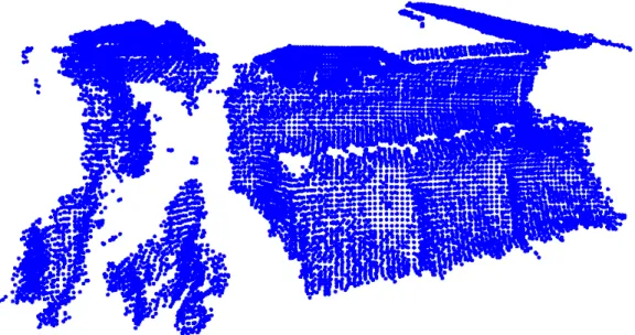
Cloud subsampling. A point cloud may contain a huge number of points in the 3D space. In order to speed up the computation, a subsampling may be performed by using the voxel down sample() function of the Open3D library, with the leaf subsampling parameter provided by the user (the higher the leaf the lower the number of extracted points). Figures 4.2 and 4.3 show how subsampling modifies an example input cloud.

2_{The SO(3) subgroup is 3-dimensional.} 3_{The domain is S}2

34 CHAPTER 4. ARCHITECTURE AND METHODOLOGIES

Figure 4.2: Example point cloud right after loading. (Cloud 0, rgbd-scenes-v2-scene 02 [17], 3DMatch dataset [36])

Figure 4.3: Same cloud as figure 4.2, after subsampling. Subsampling has been exaggerated for illustration purposes.

4.2. TRAINING DATA FLOW (FORWARD) 35 Keypoints selection. To select the keypoints, we uniformly sample the point cloud. This procedure ignores the underlying structure of the point cloud, and is employed because selecting interesting points requires an effective and general purpose 3D keypoint detector, which has not emerged yet. Indeed, this is the standard way to define keypoints when computing local descriptors. The procedure is implemented by using the same voxel down sample() function as above, with the user-specified leaf keypoints parameter: the lower the parameter and the higher the number of extracted keypoints. Figure 4.4 shows keypoints in a point cloud, sampled with a high leaf value.

Figure 4.4: Same point cloud. Keypoints highlighted with black spheres enclosing their support. During actual execution the number of keypoints is much higher and their support can be larger.

Local support extraction. For each keypoint, it is necessary to create a local point cloud that comprehends the points in the neighborhood of the keypoint itself. A radius is chosen by the user and a KDTree (from Open3D) is used to select the points within the radius. All such points are shifted in order to refer their coordinates to the position of the keypoint and achieve translation invariance. As an example, figure 4.5 shows the support of a keypoint.

Data augmentation. The local support undergoes a simple augmentation pro-cess, that consists in the application of a random 3D rotation. Since this process

36 CHAPTER 4. ARCHITECTURE AND METHODOLOGIES

Figure 4.5: Local support of a key-point from the cloud of previous fig-ures.

Figure 4.6: Local support of the same keypoint as figure 4.5, after a random sampling. The sampling has been exaggerated for illustration purposes.

is repeated each time a keypoint is extracted, the network potentially never sees the same support twice, because it will always be rotated in a different way. This is useful to increase the diversity of input data and to artificially generate differ-ent views of an object, as the real-world datasets often include a small number of different viewpoints.

Random sampling. This operation is optional. It is another form of data aug-mentation and consists in sampling with replacement a user-specified amount of points from the support, discarding the rest. It can be useful to enhance the ro-bustness of the network to clouds with lower resolutions and to acquisition noise. Figure 4.5 and 4.6 show the support of a keypoint before and after random sam-pling.

Spherical voxelization [35]. This is the most important operation, since it allows to create a spherical signal from the support points. One of the simplest methods to create a spherical signal is ray casting (see [6], figure 5): it consists in surrounding the support with a sphere, and projecting rays towards the enclosed object. As these rays touch the surface of the object, they may be used to extract