SCUOLA INTERPOLTECNICA DI DOTTORATO (SIPD)
DOCTORAL PROGRAM IN ENVIRONMENTAL AND TERRITORIAL SAFETY AND CONTROL
3D MODELING
STRUCTURES, INFRASTRUCTURES, AQUIFERS AND SHRUB
Doctoral dissertation name: Valentina Forcella
Tutor:
Prof. Luigi Mussio
The chair of the doctoral program: Prof. Fernando Sansò
3
ABSTRACT
This dissertation contributes to the 3D modeling field. In fact, the goal of this work is to obtain 3D models automatically from a discrete data set.
Each 3D model is obtained using different softwares packages and methods. The former are Fortran, Matlab, ArcGIS, Model Builder, Arcpy, and Visual Nature Studio. The latter are outlier detection, voxels, clusters analysis, feature extraction, relational matching, Delaunay triangulation, and Bruckner profiling. The order in which these methods are used depends on the data types. The input point cloud can represent a structure, an airport, an aquifer or a forest.
The study areas are five:
the China Central Television Tower Headquarters in Beijing, China an airport in Italy
the aquifer in Milan, in Italy Levy County in Florida, U.S.A. Marion County in Florida, U.S.A.
Some problems must be solved to obtain a consistent 3D model. The first problem originates from to the fact that the input data are discrete, not equally spaced or uniform and the outputted model must be continuous.
Secondly, the input information is geometric, not topological. To obtain a 3D model, topological information must be collected from the input data. Finally, if the input data contains some outliers, the predicted values will be wrong. To solve this problem, suitable procedures must be set up. Although there are other important issues, I would like to point out that this dissertation is not concerned with the different techniques available to obtain the data and to check the completeness of the data. Furthermore, this dissertation is not concerned with the rendering techniques, added light source properties, or created realistic and stylish looking models. The 3D models are obtained using Matlab ™.
1
SUMMARY
I decided to divide the summary of my dissertation into four sections: objective of the dissertation,
methodology,
problems and proposed solution, and conclusion.
1. OBJECTIVE OF THE DISSERTATION
This dissertation contributes to the 3D modeling field. In fact, the goal of this work is to obtain 3D models automatically from a discrete data set.
Some of the ideas behind this topic is that obtaining 3D models is time consuming and difficult, it requires softwares and skills and the methodology is different depending on the data type, the operator and the user.
I decided to find a general method to obtain the 3D model using different kind of point cloud. For this reason, the study cases are five and are the following:
the China Central Television Tower Headquarters in Beijing, China the Orio al Serio International airport in Bergamo, in Italy
the aquifer in Milan, in Italy Levy County in Florida, U.S.A. Marion County in Florida, U.S.A.
The data set is composed of the coordinates of the points and extra information might be included in the input data set. As mentioned, the input point cloud can represent a structure, an airport, an aquifer or a forest. The objective of the research is therefore to develop a sequence of procedures in order to obtain the 3D model automatically, independently to the type of point cloud in input.
2 To do so, some softwares packages and methods have been taken into consideration. The following sections and the dissertation provides a detailed description of each step.
2. METHODOLOGY
Each 3D model is obtained using different softwares packages and methods. The former are Fortran, Matlab, ArcGIS, Model Builder, Arcpy, and Visual Nature Studio. The latter are outlier detection, voxels, clusters analysis, feature extraction, relational matching, Delaunay triangulation, and Bruckner profiling.
In the following, a brief introduction to each software is presented.
Fortran was originally developed by IBM in 1957 for scientific and engineering applications. It is designed to allow easy translation of math formulas into code. Some eldest steps of my procedures are coded using Fortran.
MATLAB was started developing in the late 1970s by Cleve Moler, the chairman of the computer-science department at the University of New Mexico. The name MATLAB comes from MATrix LABoratory. Matrix because the data type used is the matrix, laboratory because MATLAB is used at school for didactics and research. The newest procedures, 3D models, 2D plots, and 3D plots are obtained using Matlab.
Esri's ArcGIS is a geographic information system (GIS) for working with maps and geographic information. It is used for creating and using maps, compiling geographic data, analyzing mapped information, sharing and discovering geographic information, using maps and geographic information in a range of applications, and managing geographic information in a database [Wikipedia].
Python was introduced to the ArcGIS community at 9.0. Python is a free, cross-platform, open-source programming language. ArcGIS 10 introduces ArcPy. It develops Python scripts while offering code completion and integrated documentation for each function, module, and class. In this way, only the toolbox is needed. Model builder is a way to automate a series of tools. It is a part of the ArcGIS geoprocessing framework.
Visual Nature Studio 3 makes creating complex scenes and faster rendering. Visual Nature Studio (VNS) includes foresters, engineers, landscape architects, GIS professionals, historians, graphic artists and many, many others. It is possible to import the GIS data and make a photorealistic image. The last softwares are used when the input is LiDAR data.
In the following, a brief introduction to each method and technique is presented. They are several and come from different fields. Outlier detection is a primary step towards obtaining a coherent model. Different point IDs could have the same coordinates or different points with different coordinates could have the same point ID. Some points could be out of height. The aim is to decide which points must be deleted and which one must be used.
A second method is the subdivision of the data into volumetric element. A voxel (volumetric picture element) is an element of the total volume, representing a value on a regular grid in three dimensional space [Wikipedia]. The 3D space is split by equal intervals along the three orthogonal directions to produce a voxel representation. The zero order of voxel contains 1 cube, the first order of voxel contains 8 cubes, the second one contains 64 cubes, the third one 512 cubes, the fourth one 4096 cubes, the fifth one 4096 cubes, the sixth one 32768 cubes and so on.
3 A third technique makes use of the subdivision of the data into groups. The cluster analysis is the process of organizing objects into groups whose members are similar in some way [Anderberg, 1973, Dubes and Jain, 1988] and are dissimilar to objects belonging to other clusters. Clustering algorithms may be classified in different ways.
A fourth method is the extraction of features from the point cloud. One of the possible feature is the perimeter. In fact, all the points that belong to each clusters must be perimetred with a closed loop in order to obtain a continuous 3D model. The generation of closed loops is easy only in elementary cases. It becomes more complex as the shape of the loop becomes more complicated. There are two different types of closed loops. The former is the piecewise Catmull – Rom’s lines and the latter one is the classic one.
A fifth step is the relational matching. The relational matching method is used to search the correct correspondences between points that belong to consecutive layers to generate a vertical boundary. A sixth technique is the Delaunay triangulation. It is possible to connect a set of points with triangles and triangulation is the name of this method. There are many possible triangulations, the adopted one in this dissertation is the Delaunay triangulation.
A seventh method is the interpolation, starting from the input data. The aim is to obtain a denser information. It is possible to do this using different techniques. The first one is the parametric equation of a line passing through two points. It is used to obtain the coordinates of new points. The lines are the sides obtained by Delaunay triangulation and the points are the ones of the point cloud. It is also possible to obtain the coordinates using the mean or the weight mean of the point cloud. The Bruckner diagram analysis, highly adopted in highway engineering, consists in the calculation of cut and fill volumes of soil during a road construction project. In particular, the Bruckner diagram can inform engineers about soil handling quantities to be provided or removed for each road section. Therefore, analyzing soil quantities among the whole longitudinal road profile allows the optimization of materials to be handled in order to minimize costs and hauling distances. The Bruckner diagram can be obtained by integrating the areas diagram for two consecutive road sections.
The results of the study indicate that all four types of input point cloud can be processed using the mentioned softwares package and methods. The only thinks that depends on the data type is the order in which these methods are used.
3. PROBLEMS AND PROPOSED SOLUTIONS
Some problems must be solved to obtain a consistent 3D model. The first problem originates from to the fact that the input data are discrete, not equally spaced or uniform and the outputted model must be continuous. To solve this problem, interpolating methods are used.
Secondly, the input information is geometric, not topological. To obtain a 3D model, topological information must be collected from the input data. If the shape of the model is non-stellar, to reach all the points, it is necessary to go outside the structure. If the shape of the point cloud is multi-connected, it means there is a hole. The 3D model must have the same hole. In addition, if the input point cloud has some holes, it is not possible to directly apply Delaunay triangulation and some adaptations must be done.
4 Thirdly, if the input data contains some outliers, the predicted values will be wrong. To solve this problem, suitable procedures must be set up using outlier detection tools.
Fourthly, if the input point cloud represents a concave body, Delaunay triangulation does not work so changes have to be found and applied. If the input point cloud represents a convex body, Delaunay triangulation perfectly works so no adaptations have to be done.
As mentioned in the previous section, the methods and the order they are used are the key to obtain the 3D model automatically.
As stated earlier, five different input point cloud and four different data type are taken into account. In the following, a brief scheme to the methodology adopted is described.
The first case study is a structure and is the China Central Television Tower Headquarters in Beijing, China.
I chose this building because its shape is not common and my master’s thesis case study was this one. The shape of this building is non-stellar, concave and multi–connected.
The integrated techniques and the procedures used are the following: the first one is used to check the input data set,
the second one is the “voxel” procedure that is a method based on octree encoding, the third one is called is devoted to doing the cluster analysis,
the fourth one is used to extract features from the data set, the fifth one is devoted to doing the relational matching, and
the sixth one is called “triangle” procedure and is devoted to connecting points with triangles.
The second case study is the Orio al Serio International airport, in Bergamo, Italy.
The purpose is to obtain a 3D model automatically. In addition, the area of each cross-section is required. The areas must be gotten automatically.
The applications are numerous. First of all, it is possible to re-applied this workflow to any airport independently to the Aerodrome Reference Code. Secondly, the automation of the process makes the goal of the 3D model easier and fast. Thirdly, it is possible to compare the input data with a different type of airport if the purpose is to get a new airport with a different Aerodrome Reference Code compared to the starting one.
The shape of this building is stellar, convex and single–connected.
The optimized 3D model is generated using some integrated techniques and the following procedures:
the first one is used to check the data set and to provide the first 3D plots, the second procedure is devoted to generating the 3D model,
the third one is used to analyze the input point cloud and the 3D model in terms of clusters, the fourth procedure is called “relational matching” and is devoted to connecting points
belonging to different clusters,
the fifth one is called “triangle” procedure and is devoted to connecting points with a Delaunay triangulation,
5 the sixth one is called “Bruckner” procedure and is used to evaluate the volume of soil to be
handled, and
the seventh procedure is devoted to obtaining the optimized 3D model.
The third case study is the aquifer of the city of Milan (Lombardy, north of Italy) and a nearby area of about 580 km2.
The purpose is to obtain a different workflow in case a deterministic interpolation is required. The shape of this building is stellar, convex and single–connected.
It is possible to solve the highlighted problems subdividing the data processing into six steps. First of all, the input data are checked in order to detect and remove the outliers.
Secondly, the information is divided into clusters. This procedure is carried on to assign observations into subset.
Thirdly, each cluster is interpolated using the Delaunay triangulation. This method interpolates scattered points and a continuous field is obtained.
Fourthly, closed paths between points that belong to a specific layer are built. It is necessary to bound each layer in order to know where to interpolate and where to extrapolate.
Fifthly, it is necessary to search the correct correspondences between points that belong to consecutive layers to generate the vertical boundary.
Sixthly, it is necessary to obtain new information starting from the Delaunay triangulation. This procedure is carried on using the interpolation method explained in chapter 1, section 7. The fourth and fifth case study are Levy County and Marion County. Staring from a LiDAR point cloud, the purposes of this chapter are two: the former is to obtain a better classification of the input data and the latter is to obtain density maps.
All the input points are classified into three classes: class 1 includes unclassified points, comprising vegetation, buildings, noise, etc; class 2 includes ground points; and class 9 includes water points. It is possible to better classify class 1 into new sets: roads and vegetation. This last set contains a sub-set called shrub. A shrub or bush is a woody plant characterized by several stems arising from the base and height usually under 19.658 ft (6 m) tall.
Once the shrub is detected, the idea is to cluster the shrub into subsets according to the location and the density. The shrub can be divided into three type of density: light, medium and heavy. Density maps can be used by rescuers during rescue emergency. This work can be used as the input of fire disaster pre-plan. Indeed mathematical fire behavior models require information on the location, the density and the species of each tree. Using LiDAR data, it is possible to detect the location, the height and the density, but not the species.
In order to sub-classify class 1, these different tools have to be used:
LAS to multipoints: this tool imports all the files in LAS format into a new multipoint feature class. The LAS to multipoints step is applied twice: the first time to obtain the non-ground points using the Model Builder "LAStoMPng". The second time to obtain the non-ground points using the Model Builder "LAStoMPg".
6 Point to raster: the point to raster converts point features to a raster dataset. The point to raster step is applied twice: the first time to obtain the Digital Surface Model (DSM), the second time to obtain the Digital Elevation Model (DEM).
Raster to point: the raster to point conversion tool converts a raster dataset to point features. The Raster to Point Conversion tool converts a raster dataset to point features. For each cell of the input raster dataset, a point will be created in the output feature class.
Select by attributes: it adds, updates, or removes a selection on a layer or table view based on an attribute query. To select all the points within a certain height, Select Layer By Attribute (Data Management) is used. This step is applied four times:
o vegetation high lower than 0 ft o Height between 0 ft and 3.28 ft (1 m)
o Height between 3.28 ft (1 m) and 6.56 ft (2 m) o Height between 6.56 ft (2 m) and 19.658 ft (6 m)
Split: splitting the input features, it creates a subset of multiple output feature classes. Feature to polygon: it creats a feature class containing polygons generated from areas
enclosed by input line or polygon features.
Clip: it extracts input features that overlay the clip features. This tool cuts out a piece of the roads feature class using the footprint feature in the new feature class called clipped roads. Selects features in a layer based on a spatial relationship to features in another layer.
Point density: it calculates a magnitude per unit area from point features that fall within a neighborhood around each cell.
4. CONCLUSIONS
To conclude, it is possible to obtain the 3D models automatically starting from different types of point clouds. Not only convex bodies, but also concave, non-stellar and multi-connected can be processed. The explanation and the implications to obtain the 3D model will be explained in the introduction and in the other chapters if the input point cloud represents a concave, non-stellar, and multi-connected.
I made two assumptions:
the input data is complete
the input data is obtained with different techniques, to process the data a file *.txt is required with the coordinates of the points and their IDs.
The geometric characteristics of the model are put first than the graphic output. It implies I focused my attention on how to obtain the 3D models automatically, not on the graphical restitution. I used Matlab to obtain the 3D models, fully aware there are softwares whose purpose is to renders 3D models. The models do not contain shadows, light effects, and so on.
There are some limitations. First of all, it is necessary to find out different parameters. The number of the required parameters was kept as low as possible. Different parameters are needed depending
7 on the different types of input point cloud. For this reason, different codes were written to obtain the different values automatically.
It is possible to obtain the 3D model of an input point cloud if it represents a structure, an infrastructure, an aquifer or a shrub.
It is possible to obtain the 3D model automatically using Matlab and ArcPy and scripts wrote for the purpose. It is necessary to take into account also some limitations. For example, some parameters depend on the specific input point cloud and not on the type of input point cloud.
The dissertation is divided into three parts. The first part describes contains an explanation of each technology and some modifications or alterations done in order to better apply it to the case studies. It also contains some open problems and possible solutions. Within the second section a detailed description of each study case is included. As mentioned, the study cases are:
the China Central Television Tower Headquarters (CCTV) in Beijing, China an International airport in the North of Italy
the aquifer in Milan, Italy Levy County in Florida, U.S.A. Marion County in Florida, U.S.A.
The third part contains two appendixes. The former describes an explanation of each software and the latter one describes the application in 3D of the Bézier splines. Bézier splines are defined and used in 2D space using a one coordinates. The definition of the Bézier splines in a 3D space is not available because the two coordinates that define the Bézier spline is still an open problem.
I am fully aware that I am inside a path. Some people before me studied the 3D modeling field and so will other do in the future. It is not possible to isolate works so this dissertation should be located inside a bigger workflow, made by past studies and future researches.
Although there are other important issues, I would like to point out that this dissertation is not concerned with the different techniques available to obtain the data and to check the completeness of the data. Furthermore, this dissertation is not concerned with the rendering techniques, added light source properties, or created realistic and stylish looking models.
12 CHAPTER 1
Introduction
In 3D computer graphics, 3D modeling is the process of developing a mathematical representation of any three-dimensional surface of object via specialized software. The product is called a 3D model. The model can also be physically created using 3D printing devices.
Models may be created automatically or manually. The manual modeling process of preparing geometric data for 3D computer graphics is similar to plastic arts such as sculpting. 3D models represent a 3D object using a collection of points in 3D space, connected by various geometric entities such as triangles, lines, curved surfaces, etc. Being a collection of data, 3D models can be created by hand, algorithmically, or scanned.
3D photorealistic effects are often achieved without wireframe modeling and are sometimes indistinguishable in the final form. 3D printing is a form of additive manufacturing technology where a three dimensional object is created by laying down successive layers of material. [Wikipedia]
This dissertation tries to find to answer the following questions: how is it possible to get 3D models automatically using one or few not expensive softwares? How is it possible to combine different techniques to obtain 3D model if the input point cloud represents a structure, an infrastructure, an aquifer or low vegetation?
The 3D modeling field can be split in different areas. They are the following: 3D outdoor modeling, 3D indoor modeling, 3D printing, and augmented reality. To get the goal using different techniques and softwares can be used.
It is possible to obtain 3D modeling using an application called Rhino 3D. [Gabriel Mathews]. Photosculpt Textures Software V2 will create a high definition 3D model of the subject automatically starting from two photographs. Then you can render with any 3D render.
The program generates the model within minutes simply taking two pictures of the subject. It is possible to display the model using 3D meshes. It does a great job on 3D textures and a great job on natural surfaces. [Copyright hipe0 2009].
13 A team headed by Professor Avideh Zakhor developed a laser backpack that can scan the surrounding and then it creates instantly 3D model. The goal is to obtain fast, automated, 3D model of building interiors without the human intervention.
It combines miniature lasers with an inertial unity, and cameras capture a panorama. The idea is to wear a backpack, to walk inside the building, when it is done a button is pushed and out comes the model. New breed miniature lasers with an inertial management like the one that guide missiles are used. The IMU localizes the backpack, lasers generates the geometry and four cameras generate the texture map. All three are then fused for precise navigation.
The 3D outdoor modeling combines airborne and ground-based laser scanners and cameras images. A truck equipped with one camera and two fast, inexpensive 2D laser scanners, being driven on city streets under normal traffic conditions. The Ground-based modeling and airborne modeling are merged, registered and fused in the 3D city model. [Christian Fruh and Avideh Zakhor]
A printer turns 3D models into real physical things. 3D printing will soon allow digital object storage and transportation, as well as personal manufacturing and very high levels of product customization. An example of a 3D printer is Ponoko the Makerbot. [Gabriel Mathews].
If the 3D model represents an aquifer, the 3D models of the aquifers are generated using interpretative stratigraphic sections or, more recently, the kriging technique. This last method is a stochastic one and the aim of this procedure is to estimate the value of the field at an unobserved location from a combination of the observations [Paola Gattinoni].
If the data of the input point cloud are LiDAR data, a combination of analog photointerpretation, digital softcopy photogrammetry, geographic information system (G.I.S.) and global positioning system (G.P.S.)- assisted field data collection procedures were employed in the construction of the vegetation data base. [M. Madden, Welch, T. Jordan et al.].
If the goal is to obtain a 3D model of an airport, the tools used are AutoCAD and cross-sections. Each section is joint to the previous and to the following manually. [Filippo Giustozzi].
For all these reasons, this dissertation tries to find an almost unique workflow to obtain automatically the 3D model. The goal is also to be able to repeat the modeling on the same type of input point cloud but, for example, in a different location.
The previous solutions adopted have some limitations and some problems must be solved.
For example, Photosculpt Textures Software V2 is only useful for textures with bump maps, not entire buildings or mountains. It does not work 360 degree perfectly.
Another problem is the following: many people may do not want or be able to afford a 3D printer. Prices for most commercial/industrial 3D printers tend to start in the ten-to-twenty thousand dollar bracket and spiral upwards.
Using a stochastic method to interpolate data, the value estimated in a point where the measure was acquired does not coincide with the measure itself.
Achieving the 3D model of the airport through the manually cross sections is time consuming and the repeatability is missing.
So far no one has investigated the link between different methods and few softwares to obtain 3D models automatically. And even using well-known technology, such as Delaunay triangulation, some problems must need to be solved. In fact, the above-mentioned solution do not apply to a concave body case.
Also the Bruckner profiling is a well-know methodology, but it is not possible to apply it to an airport without drawing cross section manually.
14 To conclude, the purposes are two: the first one is the outputted automatic 3D model and the repeatability of the process.
I divided my dissertation into three parts. The first one contains an explanation of each technology and some modifications or alterations done in order to better apply it to the case studies. It also contains some open problems and possible solutions.
Within the second section a detailed description of each study case is included. As mentioned in the summary, the study cases are:
the China Central Television Tower Headquarters (CCTV) in Beijing, China an International airport in the North of Italy
the aquifer in Milan, Italy Levy County in Florida, U.S.A. Marion County in Florida, U.S.A.
The fist one is used to obtain a proper workflow for a structure. The CCTV was chosen because of its unusual shape.
The second study case was chosen because a previous study on that airport was done in the Infrastructure department at Politecnico di Milano, in Italy.
The third study case is the aquifer in Milan and a nearby area of about 580 km2. A previous model was done by Gattinoni.
The fourth and fifth case studies are Levy County and Marion County in Florida, U.S.A. I spent six months at the Center for Geospatial Research (CGR), formerly the Center for Remote Sensing and Mapping Science (CRMS). Doctor Marguerite Madden is the Director of the Center for Geospatial Research and Doctor Jordan, Thomas R. is the Associate Director of the Center for Geospatial Research.
The third part contains two appendixes. The former describes an explanation of each software and the latter one describes the application in 3D of the Bézier splines. Bézier splines are defined and used in 2D space using a one coordinates. The definition of the Bézier splines in a 3D space is not available because the two coordinates that define the Bézier spline is still an open problem.
15 CHAPTER 2
Techniques
This chapter explains the different techniques used to obtain 3D models automatically. They are several techniques and they come from different fields.
The techniques used and their order depend on the input data type. In fact, the input point cloud can represent a structure, an airport, an aquifer or shrubs.
The following list provides the name of the techniques utilized: outlier detections, voxel distribution, cluster analysis, relational matching, features extraction, Delaunay triangulation, interpolation,
Brückner profiles, and stabilized Erone.
For each method at least one applied example is provided. The proposed examples are a structure, an airport and an aquifer.
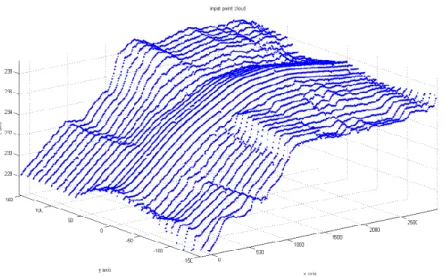
The first one is a not an existing building, but it resembles a derrick and a frame structure. The shape of this case study is complex because it is concave, non-stellar, and multi-connected. This building is used to test multiple software programs I wrote using Matlab and Fortran. Figure 2.1 shows the point cloud that represents the building.
16 Figure 2.1 Structure: input point cloud
The second one is an airport and is also analyzed in chapter 7. An airport is composed of several parts. They are the Clear Way, RESA, center line, runway, runway shoulders, Cleared and Grated Area (CGA) and runway strip.
Figure 2.2 shows the point cloud that represents the airport.
Figure 2.2 Airport: input point cloud
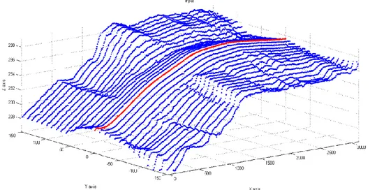
The third study case is the aquifer, which is also used for the study case in chapter 8. The aquifer is modeled by points defined by three coordinates and the type of layer to which they belong. There are four different layers:
land surface layer, Aquitard up layer,
Aquitard down layer, and Aquiclude layer.
17 Figure 2.3 Aquifer: input point cloud
Each method is explained in detail in sections 1.1 to 1.9.
2.1. OUTLIER DETECTION
Outliers are values that are numerically distant from the rest of the data and must be recognized and might be excluded from further data analysis [V. Pupovac and M. Petrovečki]. The presence of outliers can dramatically change the shape of 3D model. For this reason, it is necessary to remove the outliers from the input point cloud.
Detecting and correcting outliers automatically is impossible because there are many kinds of outliers and their presence is different in each input point cloud. Nevertheless, I found three kinds of outliers in the input point clouds I analyzed.
First of all, different point IDs could have the same three coordinates. Second, different points with different coordinates could have the same point ID. Lastly, some points could be anomalies.
The aim is to decide which points must be deleted and which one must be processed, independently from the type of outliers.
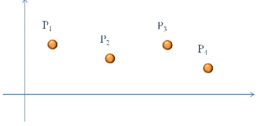
A short example will clarify the adopted procedure: there are five points in figure 2.4. The points P2
18 Figure 2.4 First type of outliers
Only one of the two points is processed, as shown in the following picture.
Figure 2.5 Points after outlier detection
The second kind of outlier is the following: different points with different coordinates have the same point ID. In this case, the point ID of one of these points is changed.
In figure 2.6 the third kind of outlier is shown. There are seven points and the point P7 is classified
as belonging to the same point cloud. That point is an outlier.
Figure 2.6 Points before the outlier detection
2.2. VOXELS
A voxel (volumetric picture element) is an element of the total volume, representing a value on a regular grid in three dimensional space [Wikipedia].
As a pixel represents the information about a 2D field, a voxel is the equivalent in the 3D world. Voxels are used for analysis and visualization of 3D-dimensional distribution of data.
The 3D space is split by equal intervals along the main orthogonal to produce a voxel representation.
19 Figure 2.7 Voxel
The number of voxels used in a calculation can vary.
The optimal data allocation is reached through division of the whole data set into data subsets and keeping only non-zero pieces of data in memory.
It is possible to start the subdivision into voxels using the maximum dimensions of the scene to adjust the dimensions of the starting cube. Then the starting cube is subdivided into 8 volumes. Each new volume is subdivided into 8 volumes if the starting volume is not empty. This procedure goes on until the volumes are empty.
The procedure described in the three steps imply the fact that the zero order of voxel contains 1 cube, the first order of voxel contains 8 cubes, the second one contains 64 cubes, the third one 512 cubes, the fourth one 4096 cubes, the fifth one 4096 cubes, the sixth one 32768 cubes and so on. The following pictures show the starting volume, and then subdivided into different order of voxels. Figure 2.8 shows the sub-division of the input point cloud into the zero order of voxel. There is only 1 cube.
Figure 2.8 Voxel, 0° order
In this case the amplitude in x is equal to xmin – xmax, the amplitude in y is equal to ymin – ymax, and the amplitude in z is equal to zmin – zmax.
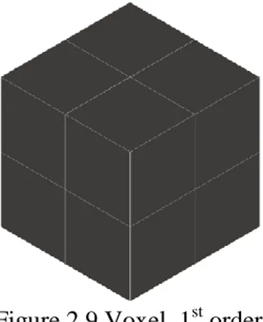
Figure 2.9 shows the sub-division of the input point cloud into the first order of voxel. There are 8 cubes.
20 Figure 2.9 Voxel, 1st order
In this case the amplitude in x is equal to xmin – xmax divided by 2, the amplitude in y is equal to ymin – ymax divided by 2, and the amplitude in z is equal to zmin – zmax divided by 2.
Figure 2.10 shows the sub-division of the input point cloud into the second order of voxel. There are 64 cubes.
Figure 2.10 Voxel, 2nd order
In this case the amplitude in x is equal to xmin – xmax divided by 4, the amplitude in y is equal to ymin – ymax divided by 4, and the amplitude in z is equal to zmin – zmax divided by 4.
Figure 2.11 shows the sub-division of the input point cloud into the first order of voxel. There are 512 cubes.
21 In this case the amplitude in x is equal to xmin – xmax divided by 8, the amplitude in y is equal to ymin – ymax divided by 8, and the amplitude in z is equal to zmin – zmax divided by 8.
Figure 2.12 shows the sub-division of the input point cloud into the first order of voxel. There are 4096 cubes.
Figure 2.12 Voxel, 4th order
In this case the amplitude in x is equal to xmin – xmax divided by 32, the amplitude in y is equal to ymin – ymax divided by 32, and the amplitude in z is equal to zmin – zmax divided by 32.
Most literature seems to point to an Octree as the most suitable structure for a hierarchical structure of a voxel grid. There are two kinds of algorithms for ray-octree intersection: bottom-up, which works from the leaves back upwards, and top-down, which is basically a depth-first search.
This enables spatial partitioning, down sampling and search operations on the point data set. Each octree node has either eight children or no children. The root node describes a cubic bounding box which encapsulates all points. This representation is shown in figure 2.13.
Figure 2.13 Octrees
A generalization of voxels is doxels, or dynamic voxel. This is used in the case of a 4D dataset, for example, an image sequence that represents 3D space together with another dimension such as time. It allows the representation and analysis of space-time systems.
There are efficient methods for creating a hierarchical tree data structure from point cloud data. The aim of this technique is to estimate the three values needed afterwards too. For each order of voxel, a list provides:
22 the voxel ID, and
the number of points that belong to that voxel.
This procedure continues up to the order in which the voxels are all empty. Another list contains only the full voxels, their full-voxel ID, their voxel ID and the number of points that belong to that full voxel.
The 3D output plot given is characterized by different colors, one for each order. The meaning of the different colors is the following one:
cyan is used for the points classified as belonging to voxel 1°, black is used for the points classified as belonging to voxel 2°, yellow is used for the points classified as belonging to voxel 3°, blue is used for the points classified as belonging to voxel 4°, red is used for the points classified as belonging to voxel 5°, green is used for the points classified as belonging to voxel 6°, and purple is used for the points classified as belonging to voxel 7°.
The next part contains the description of the application of the voxel procedure to the structure. The following figure shows the input point cloud.
Figure 2.14 Input point cloud
The example body is composed of 469 points. The xmin is equal to - 40.000 m, the xmax is equal to 110.000 m, the ymin is equal to 40.000 m, the ymax is equal to 70.000 m, the zmin is equal to -20.000 m, and the zmax is 150.000 m.
Voxel 0° is composed of one cube and it contains all the 469 points.
Voxel 1° is subdivided into 8 cubes. The following table provides for each cube the number of points inside.
# cubes 1 2 3 4 5 6 7 8
23 Table 2.1 Voxel 1st order
Because none of the cubes are empty, the voxel subdivision will go on till the sixth order.
The 3D output plot given is characterized by different colors, one for each order. The meaning of the different colors is the same already mentioned.
Figure 2.14 Voxel distribution
2.3. CLUSTER ANALYSIS
Clustering is the process of organizing objects into groups whose members are similar in some way [Anderberg, 1973, Dubes and Jain, 1988] and are dissimilar to objects belonging to other clusters. A simple graphical example is shown it the following figures. The former shows the unlabeled data and the points are in black.
Figure 2.15 Starting points
24 Figure 2.16 Clustered points
In this case the 8 clusters into which the data can be divided are easily identified using a similarity criterion (distance).
What constitutes a good clustering? For a successful outcome, the criterion used is dependent on the type of clustering that is sought after.
Clustering algorithms may be classified in differently; therefore different techniques can be used. They are the following:
bottom – up, top – down,
exclusive clustering, and overlapping clustering.
The first type of classification depends on the initial number of clusters. It may be equal to the number of data (bottom - up) or equal to one (top - down).
The second type of classification depends on the fact that a datum may belong to a single cluster (exclusive cluster) or to multiple clusters (overlapping clusters).
2.3.1. Bottom – up technique
The first type of cluster technique is the bottom – up technique. At the beginning all the points are classified as a single cluster. Then the algorithm merges the nearest clusters. This step will go on until the number of clusters reaches a prearranged value or till the minimum distance between the clusters does not exceed a fixed threshold.
2.3.2. Top – down technique
The second type of cluster technique is the top – down technique. At the beginning all the points are classified as belonging to the same cluster. Then the algorithm divides the starting cluster into different clusters. This step will go on until the number of clusters reaches a prearranged value.
2.3.3. Exclusive clustering
The third type of cluster technique is the exclusive technique.
Data are grouped in an exclusive way, so that if a certain datum belongs to a definite cluster then it could not be included in another cluster. A simple example of that is shown in the figure 2.17 below, where the separation of points is achieved by the straight line in black.
25 Figure 2.17 Exclusive clusters
This type of clustering algorithm is also known as hard clustering. 2.3.4. Overlapping clustering
The fourth type of cluster technique is the exclusive technique.
The overlapping clustering uses fuzzy sets to cluster data, so that each point may belong to two or more clusters with different degrees of membership. In this case, data will be associated to an appropriate membership value. A simple example of that is shown in the following figure, where the separation of points is achieved by overlapping circles.
Figure 2.18 Overlapping clusters 2.3.5. Others
Another type of clustering is also known as soft clustering or fuzzy clustering.
The third type of classification depends on the type of algorithm used to separate the space. There are three types of clustering algorithms:
partitioning, hierarchical, and density algorithms.
Each classification will be explained in detail in the following sections. 2.3.5.1. Partitioning algorithms
The partitioning algorithm typically starts with an initial partition of and then uses an iterative control strategy to optimize an objective function. A two-step procedure is used. First, determine
26 representatives minimizing the objective function. Second, assign each object to the cluster with its representative “closest” to the considered object. The second step implies that a partition is equivalent to a Voronoi diagram and each cluster is contained in one of the Voronoi cells.
K-means clustering is a method in which each observation belongs to the cluster with the nearest mean.
The term "k-means" was first used by James MacQueen in 1967, though the idea goes back to Hugo Steinhaus in 1957. The standard algorithm was first proposed by Stuart Lloyd in 1957 as a technique for pulse-code modulation, though it was not published until 1982.
These centroids should be placed in a cunning way because a different location can cause a different result. So, the better choice is to place them as far away from each other as possible.
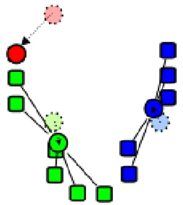
The following example shows 15 point that need to be divided into three subsets. The k initial "means" are randomly selected from the data set. In picture number 2.19 the 3 points are displayed with circles, the others with squares.
Figure 2.19 Three points chosen as centroids
K clusters are created by associating every observation with the nearest mean. The partitions represent the Voronoi diagram generated by the means. It is displayed in the following pictures.
Figure 2.20 Three different areas
At this point k new centroids are re-calculated as barycenters of the clusters resulting from the previous step. In the following picture the new centroids are displayed with circles.
27 Figure 2.21 Three new centroids
After these k new centroids are found, a new binding has to be done between the same data set points and the nearest new centroid. The previous two steps are repeated until convergence has been reached. The result is displayed in figure 2.22.
Figure 2.22 Final result The k-means are represented with circles, the others with squares.
Although it can be proved that the procedure will always terminate, the k-means algorithm does not necessarily find the most optimal configuration, corresponding to the global objective function minimum. The algorithm is also significantly sensitive to the initial randomly selected cluster centres. The k-means algorithm can be run multiple times to reduce this effect.
2.3.5.2. Fuzzy C-means
This method was developed by Dunn in 1973 and improved by Bezdek in 1981.
Fuzzy c-means (FCM) is a method of clustering which allows one piece of data to belong to two or more clusters. This method is frequently used in pattern recognition. It is based on minimization of the following objective function:
where is any real number greater than 1, is the degree of membership of in the cluster ,
is the ith of d-dimensional measured data, is the d-dimension center of the cluster, and is any norm expressing the similarity between any measured data and the center.
28 2.3.5.3. Quality Threshold
Quality Threshold is an algorithm that groups data into high quality clusters. Quality is ensured by finding large cluster whose diameter does not exceed a given user-defined diameter threshold. This method prevents dissimilar data from being forced under the same cluster.
The following steps provides the sequence that must be followed: 1. A random datum is chosen from the selected datum list.
2. The algorithm determines which datum has the greatest similarity to this gene. If their total diameter does not exceed the diameter threshold, then these two data are clustered together. 3. Other data that minimize the increase in cluster diameter are iteratively added to this cluster.
This process continues until no datum can be added to this first candidate cluster without surpassing the diameter threshold.
4. A second candidate datum is chosen.
5. The algorithm determines which data has the greatest similarity to this second gene. All data in the selected gene list are available for consideration to the second candidate cluster.
6. Other data from the selected datum list that minimize the increase in cluster diameter are iteratively added to the second candidate cluster. The process continues until no datum can be added to this second candidate cluster without surpassing the diameter threshold.
7. The algorithm iterates through all data on the selected gene list and forms a candidate cluster with reference to each gene. In other words, there will be as many candidate clusters as there are data in the data list. Once a candidate cluster is formed for each data, all candidate clusters below the user-specified minimum size are removed from consideration.
8. The largest remaining candidate cluster, with the user-specified minimal number of datum member, is selected and retained as a QT cluster. The data within this cluster are now removed from consideration. All remaining data will be used for the next round of QT cluster formation. 9. The entire process is repeated until the largest remaining candidate cluster has fewer than the
user-specified number of genes.
10. The result is a set of non-overlapping QT clusters that meet quality threshold for both size, with respect to number of data, and similarity, with respect to maximum allowable diameter.
11. Data that does not belong in any clusters will be grouped under the “unclassified” group. 2.3.5.4. DBSCAN
DBSCAN (for density-based spatial clustering of applications with noise) is a data clustering algorithm proposed by Martin Ester, Hans-Peter Kriegel, Jörg Sander and Xiaowei Xu in 1996. It is a density-based clustering algorithm because it finds a number of clusters starting from the estimated density distribution of corresponding nodes.
When looking at the sample sets of points depicted in figure 2.23, it is possible to detect clusters of points and noise points not belonging to any of those clusters.
29 Figure 2.23 Samples
The main reason why it is possible to recognize the clusters is that within each cluster, a typical density of points is considerably higher than outside of the cluster. Furthermore, the density within the areas of noise is lower than the density in any of the clusters.
Different colors in the following picture represent the different clusters.
Figure 2.24 Clustering discovered by DBSCAN
A cluster obtained with DBSCAN technique satisfies the following two properties: 1. all points within the cluster are mutually density-connected and
2. if a point is density-connected to any point of the cluster, it is part of the cluster as well. DBSCAN requires two parameters:
ε and
minPts: the minimum number of points required to form a cluster [Wikipedia].
It starts with an arbitrary starting point that has not been visited. This point's ε -neighborhood is retrieved, and if it contains sufficiently many points, a cluster is started. Otherwise, the point is labeled as noise. Note that this point might later be found in a sufficiently sized ε -environment of a different point and hence becomes part of a cluster.
If a point is found to be a dense part of a cluster, its ε -neighborhood is also part of that cluster. Hence, all points that are found within the ε neighborhood are added, as is their own ε -neighborhood when they are also dense. This process continues until the density-connected cluster is completely found. Then, a new unvisited point is retrieved and processed, leading to the discovery of a further cluster or noise.
30 Figure 2.25 DBSCAN can find non-linearly separable clusters. This dataset cannot be adequately
clustered with k-means or EM clustering.
Figure 2.26 Another comparison between k-means and DBSCAN.
The adopted cluster technique is a top – down and exclusive one. Different methods are used, depending on the different types of input point cloud.
It is possible to apply the cluster analysis in three different ways: to cluster the data vertically,
to cluster the data horizontally, and
to cluster to data depending on the characteristic of the points themselves inside the point cloud.
The first kind of cluster analysis is applied using the first parameter estimated using the “voxel” procedure. For each level, the information is listed in this way:
vertical cluster ID,
number of points belonging to that vertical cluster, height, and
ID point at that level.
The following table provides an example of the output:
Vertical cluster ID # of points Height (m) Point IDs
31 … 60 87 68 … 52 8 150.000 272 277 276 … 279 278 275 Table 2.5 Vertical clusters
The next part contains the description of the application of the cluster analysis procedure to the structure. One 3D plot for each vertical cluster is provided and one 3D plot for the input point cloud. The former are displayed in figure 2.27 and the latter in figure 2.28.
32
Figure 2.27 Vertical clusters
The following picture displays the 3D plot containing all the vertical clusters. The alternation of colors from red to blue represents the switch from one vertical cluster to the next.
Figure 2.28 Vertical clusters There are 18 vertical clusters.
The second kind of cluster analysis is applied using the second parameter estimated using the “voxel” procedure. In order to generate contours, finite point sets at each level must be constructed. These sets could involve all points belonging to a level, or there could be different sets at the same level, if necessary.
Each horizontal cluster is described by: horizontal cluster ID,
33 its height,
the point ID belongs to the horizontal cluster, and
the number of points that belong to the horizontal cluster. The following table provides an example of the output:
Horizontal cluster ID Height (m) Point IDs # of point
1 -20.000 401 402 413 132 476 519 525 … 22 150.000 272 277 276 9 278 279 285
Table 2.6 Horizontal clusters
The number of 3D plots is equal to the number of vertical clusters. In fact, if a vertical cluster contains more than one horizontal cluster, the 3D plot contains all the horizontal clusters at that level.
The following pictures show the horizontal clusters. If the vertical cluster contains one horizontal cluster, the points are displayed in red. If the vertical cluster contains more than one horizontal cluster, the points are displayed with different colors, one for each horizontal cluster.
35 Figure 2.29 Horizontal clusters
In this study case there are 22 horizontal clusters.
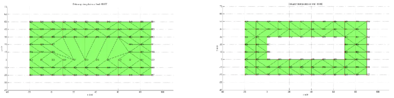
The third kind of cluster analysis is applied to data depending of their characteristics. As mentioned earlier, in chapter 7 I will explain how it is possible to obtain the 3D model of an airport. It is necessary to cluster the input point cloud into different sets, depending on what the acquired points represent from an actual airport.
In the airport study case, figure 2.30 shows the image “InputSets.tif” with two different colors: the center line (first set) is in red and the other points (second set) are in blue.
Figure 2.30 Center line in red and the other points in blue
The dimension of each part depends on the Aerodrome Reference Code. This code prescribes the widths and the cross slopes. Through this information, it is possible to cluster the input point cloud. Figure 2.31 shows the results of the cluster analysis.
Red is used for the points classified as belonging to the center line cluster, Blue is used for the points classified as belonging to the runway cluster,
Green is used for the points classified as belonging to the runway shoulders cluster, Black is used for the points classified as belonging to the Clear and Grated Area cluster, Purple is used for the points classified as belonging to the runway strip cluster, and Yellow is used for the points classified as belonging to the last cluster.
36 Figure 2.31 Clustered input point cloud
The following table provides an example of the output:
Point ID X Y Height (m) Cluster ID
…
4942 90.34692125 89.54085275 228.53600000 2 4943 101.52819376 89.81579838 228.654 2
…
Table 2.7 Cluster analysis
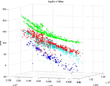
As mentioned, I will explain how it is possible to obtain the 3D model of an aquifer in chapter 8. It is necessary to cluster the input point cloud into different sets.
The aquifer is divided into four layers: this information is used to divide the data into clusters. The following image shows the clusters using four different colors:
green for the points classified as belonging to the land surface layer, red for the points classified as belonging to the aquitard up layer,
light blue for the points classified as belonging to the aquitard down layer, and blue for the points classified as belonging to the aquiclude layer.
37 Figure 2.32 Cluster analysis of the aquifer
2.4. FEATURE EXTRACTION
It is possible to extract different types of information from the point cloud. Also, it is possible to extract the perimeter of each horizontal cluster and to classify the type of each horizontal cluster. It is necessary to obtain the perimeter in order to know where it is necessary to interpolate and where to extrapolate information.
There are different kinds of perimeters; here I will present two of them. The first is the classic one and the second is the piecewise Catmull – Rom’s lines. The classic one is used in case the study case is characterized by rough edges; the piecewise Catmull – Rom’s lines in the opposite case. There are different types of horizontal cluster. Here the attention is focused on the classification based on the distinction between sowns and chains.
A sown is the representation of a horizontal plane formed by dense points. A chain is a planar path modeled by rare points. Figure 2.33 shows a chain with blue dots and a sown with red dots.
Figure 2.33 Chain (left) and sown (right) The following table provides an example of the output:
Horizontal cluster ID Height (m) Type
38
10 40.000 Chain
11 50.000 Chain
…
Table 2.8 distinction between chains and sowns
This distinction is done because the different type of horizontal cluster affects both the relational matching and the Delaunay triangulation.
I will explain the relational matching in section 5 and the Delaunay triangulation in section 6. Here I will explain the connection between the type of horizontal cluster and the two techniques.
If the relational matching is done between a chain and a sown, the number of matched points is different because a chain and a sown are composed of a different number of points.
If the relational matching is carried on between two chains, it connects each point of the former one with each point of the latter one.
A brief introduction about the perimeter technique will be followed by a detailed description of the two different kinds of perimetrations.
2.4.1. Perimeter
In order to obtain a continuous 3D model, all the points that belong to each cluster must be perimetred with a closed loop.
A perimeter is a path that surrounds an area or a path that connects a group of points. The word comes from the Greek peri (around) and meter (measure).
The generation of closed loops is easy only in elementary cases. It becomes more complex as the shape of the loop becomes more complicated. In order to implement this part of the research, the reconstruction of a four letters (F, G, R, and W) and a spider shape was preliminarily performed, starting from the raw points.
The next images show the shapes analyzed.
39 Figure 2.35 Point cloud for letter G
Figure 2.36 Point cloud for letter R
40 Figure 2.38 Point cloud for a spider shape
To find a closed loop, first the software connects a point to its closest point; next it connects this second point to its closest (excluding the first) and so forth (in order to keep a unique sense of advancement). At this step, a certain number of points will not be connected to the others. Isolated points must be connected in a different hierarchic way:
with the first point, listed in the previous, with the last one, in the same list,
with all the remaining points, and
with all the ones selected, in the meantime.
Subsequently, isolated loops are connected. Typically these points belong to levels, separated by a unique level, quite often consisting in one or a few points.
Only at this step, it is possible to follow the path of the loop. Indeed following a level structure, the path between its root and the farthest leaf identifies the first half of the loop. The second part is done attempting to reach the root starting from the farthest leaf.
In some cases, it is really impossible to reach the root. Therefore, the whole path is formed by adding single steps, starting from the point where the previous step finishes. At the end, when all points have been taken into account, all the sides not used will be deleted, because lying inside the closed loop they are useless.
Figure 2.39 shows the 14 input points.
41 The solution showed in figure 2.40 is wrong because the perimeter is not closed. The closed loop is a path whose initial point is equal to the terminal point. Contour #1 starts in P1 and finishes in P2. It
is therefore wrong.
Figure 2.40 Contour #1
All the points must be taken. Contour #2 does not contain P5, P8, P11, and P14.
Figure 2.41 Contour #2
All the points must be taken only once. Contour #3 takes P4, P6, P8, P9, and P10 at least two times. It
is therefore wrong.
42 All sides, if taken, only once and they do not have to cross each other. Contour #4 is therefore wrong.
Figure 2.43 Contour #4 Contour #5 is the correct one.
Figure 2.44 Contour #5
The follow three images show the closed loops of the other letters analyzed.
43 Figure 2.46 Contour, letter G
Figure 2.47 Contour, letter W
There are two different types of closed loops. The first is the piecewise Catmull – Rom’s lines, the second type is the classic one. The following two paragraphs contain a description of the two different techniques.
2.4.2. Piecewise Catmull – Rom’s lines
It is possible to continuously model every loop with piecewise Catmull – Rom’s lines and, starting from 3 points, every straight line passes through the second point and it is parallel to the line joining the first and the third points.
The following image shows an example of 5 input points.
Figure 2.48 Five input points
44 Starting from points P1, P2 and P3, the straight line (in light blue in figure 2.49) is parallel to the line
joining the points P1 and P3.
Figure 2.49 First line of the Catmull – Rom closed loop
The first straight line passes through point P2 and it is parallel to the line joining the point P1 and P3.
See figure 2.50 for a better representation.
Figure 2.50 First line of the Catmull – Rom closed loop
The same method is applied to the other four sides. The perimeter is obtained. This image shows the Catmull-Rom closed path between the 5 input points.
Figure 2.51 Perimeter with Catmull – Rom
The advantage of this type of interpolation is the possibility to extrapolate other information. It is possible to evaluate:
45 the two coordinates of each new points (in blue in figure 2. x) and
for each straight line (in orange in figure 2.x): o type of straight line:
in the first case, a y is displayed in the second, an x is displayed o the slope of the straight line and
o y-intercept or x-intercept.
Figure 2.52 Catmull – Rom closed loop (in orange), the five input points (in light blue) and the five new points (in blue)
The first table refers to the new points (in blue in the picture 2.52). The second table refers to the sides (in orange in the picture 2.52).
Points
Interpolation ID Horizontal cluster ID Point ID X Y Z
1 1 5001 0.000 0.000 0.000 … … … … Table 2.9 Points Lines Interpolation ID Horizontal cluster ID Side ID Point ID Type of line Slope x-intersect or y-intersect 1 1 1 1 2 3 y 0.000 0.000 2 2 3 4 y 0.000 0.000 … … … … Table 2.10 Lines
The piecewise Catmull-Rom lines perimeter is used in case the structure is characterized by smooth edges. An example of this kind of structures is designed by the architect Zaha Hadid. An example of her futuristic building is the Defunct Factory in downtown Belgrade and a picture of this building is in the following figure.
46 Figure 2.53 Beko Building, Zaha Hadid
If this perimetration is set, the following step uses Bézier splines. They will be explained in the appendix.
2.4.3. Classic way
It is also possible to model every loop in the classic way, in order to make a comparison between the two modes (Catmull-Rom and the classic way).
The following image shows the classic contour between the same five points displayed in figure 2.53.
Figure 2.53 Classic perimeter
The Delaunay triangulation will be explained in subchapter 6. It is here mentioned because it is possible to extract the close loop from the Delaunay triangulation if the structure is convex.
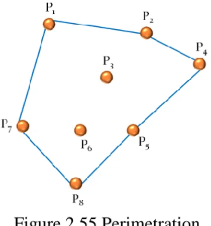
In order to do this, a short example will clarify the adopted procedure. The following picture (Figure 2.54) shows an example of Delaunay triangulation between eight points. There are fourteen sides.
47 Figure 2.54 Triangulation
Each triangle is composed of three sides. If a side is in common with more than one triangle, it is deleted. On the contrary, the side is classified as a side of the closed path.
The sides P1 – P3, P2 – P3, P4 – P3, P5 – P3, P5 – P6, P8 – P6, P7 – P6, P1 – P6, and P6 – P3 belong to
more than one triangle. These sides are deleted and the contour is obtained. The following picture (Figure 2.55) shows the result.
Figure 2.55 Perimetration
It is not possible to obtain the closed loop starting from the Delaunay triangulation if the body/structure/horizontal cluster is concave.
Figure 2.56 provides the 14 points that represent the “F” and its triangulation.
Figure 2.56 Delaunay triangulation
48 Figure 2.57 Perimetration
Figure 2.58 shows the correct perimetration.
Figure 2.58 Perimetration 2.4.4. Type: chain or sown?
As mentioned, it is necessary to classify a horizontal cluster in a chain cluster or a sown cluster. In fact, a structure can be composed of two different sets of information: sowns and vertical or almost vertical walls.
The information is provided in the following way: horizontal cluster ID,
type of clustres, and height.
The following table provides the classification of each horizontal cluster.
Horizontal cluster ID Type Height (m)
1 sown -20.000 2 sown -10.000 3 sown 0.000 4 chain 10.000 5 chain 10.000 6 chain 20.000 7 chain 20.000 8 sown 30.000
49 9 chain 40.000 10 chain 40.000 11 chain 50.000 12 chain 50.000 13 sown 60.000 14 chain 70.000 15 sown 80.000 16 sown 90.000 17 chain 100.000 18 chain 110.000 19 chain 120.000 20 chain 130.000 21 chain 140.000 22 chain 150.000
Table 2.11 Feature extraction
Figure 2.60 displays the point cloud with two colors: green if the horizontal cluster represents a sown, blue if it is classified as a chain.
Figure 2.60 Chains (in blue) and sowns (in green)
2.5. RELATIONAL MATCHING
Relational matching is a method for finding the best correspondences between data to generate a vertical boundary.
Matching algorithms may be analyzed by posing three fundamental questions: what kind of data is matched?
what is the best match?
how to find the best match? [Lecture notes in computer science, 628]
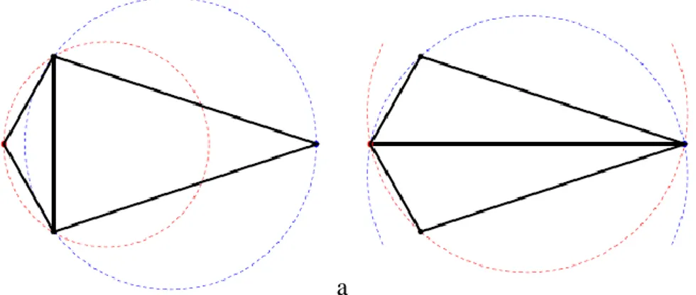
50 The relational matching method is used to search the correct correspondences between points that belong to consecutive layers to generate a vertical boundary. Figure 2.61 shows two sets of points that belong to different but consecutive levels in orange and the two perimeters in light blue.
Figure 2.61 Points and contours
The first proposed solution in figure 2.62 is wrong and the consistency of matched sides is missing.
Figure 2.62 First solution
In order to obtain the best match, the connections must satisfy the following properties:
the points in question must be as close as possible while still belonging to consecutive clusters,
if points belong to the same vertical, they are easily matched, and
if not, the software looks to create connections along the same direction [Forcella, Mussio, Reconstructing CCTV 2011].
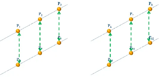
The above mentioned “same direction” can be almost vertical or almost horizontal. I will provide two examples to create a better understanding of the technique and the results.
Picture 2.63 shows the correct relational matching between the 20 points showed in figure 2.47. These points are connected using the vertical direction.