Scuola di Ingegneria e Architettura
Dipartimento di Informatica - Scienza e Ingegneria (DISI)
Corso di Laurea Magistrale in Ingegneria Informatica
Tesi di Laurea
in
Computer Vision and Image Processing
Deep Learning Techniques applied to
Photometric Stereo
Candidato:
Federico Domeniconi
Relatore:
Prof. Luigi Di Stefano
Correlatori:
Ing. Pierluigi Zama Ramirez
Ing. Andrea Campisi
I would first like to thank professor Luigi Di Stefano and my two tutors, Pierluigi Zama Ramirez and Andrea Campisi, for their advice and for guiding me in the
development of this thesis.
I would also like to thank all the T3Lab guys that have been great companions during the internship and made my experience really enjoyable.
Last but not least, I wish to express my deepest gratitude to my brother, my parents and all my friends for supporting me during this period.
The thesis is focused on the study of state-of-the-art deep learning photo-metric stereo: the Self-calibrating Deep Photophoto-metric Stereo Networks. The model is composed of two networks, the first predicts light directions and intensities, the second predicts the surface normals. The goal of the thesis is to understand the model limitations and to figure out if it can be adjusted to perform well also on real-world scenarios. The thesis project is based on fine-tuning, a supervised transfer learning technique. For this purpose a new dataset is created by acquiring images in laboratory. The ground-truth is obtained by means of a distillation technique. In particular the light di-rections are gathered using two light calibration algorithms and combining the two results. Similarly the normal maps are gathered combining the re-sults of various photometric stereo algorithms. The rere-sults of the thesis are really promising. The prediction error of light direction and intensities is one third of the original model’s error. The predictions of surface normal can be analyzed only qualitatively, but the improvements are clear. The work of this thesis showed that is possible to apply transfer learning to deep learning photometric stereo. Thus it is not necessary to train a new model from scratch but it is possible to take advantage of already existing models to improve the performance and reduce the training time.
1.1 Example of photometric stereo . . . 4
1.2 Vectors defined in Woodham’s algorithm . . . 6
1.3 Comparison of diffuse and specular reflectance . . . 8
1.4 Comparison of attached and cast shadows . . . 9
2.1 Perceptron flowchart . . . 13
2.2 Structure of a convolutional neural network . . . 15
2.3 Example of convolution operation . . . 16
3.1 The setup used for the images acquisition . . . 20
3.2 Reference object for the first method of light calibration . . . 21
3.3 Reference object for the second method of light calibration . . . 21
3.4 Different views of the results of the two calibration algorithm . . . . 22
3.5 Some of the objects in the dataset part 1 . . . 23
3.6 Some of the objects in the dataset part 2 . . . 23
3.7 Some of the objects in the dataset part 3 . . . 24
4.1 Self-calibrating Deep Photometric Stereo Networks structure . . . . 28
4.2 Example of output of the algorithms and the average result . . . 41
4.3 Example of discordance matrix . . . 44
4.4 Functions used to generate loss weights . . . 45
5.1 Egg shaped object normal maps output example 1 . . . 49
5.2 Egg shaped object normal maps output example 2 . . . 50
5.3 Coffee cup normal maps output example 1 . . . 50
5.4 Coffee cup normal maps output example 2 . . . 51
4.1 Grid search for hyperparameters tuning . . . 36
4.2 Layers freezing . . . 38
4.3 Model configuration . . . 39
4.4 Computation of the normal map ground-truth . . . 42
4.5 Computation of the discordance matrix . . . 44
INTRODUCTION 1 1 PHOTOMETRIC STEREO 3 1.1 DESCRIPTION . . . 3 1.2 WOODHAM’S ALGORITHM . . . 3 1.2.1 HYPOTHESIS . . . 5 1.2.2 THE ALGORITHM . . . 5 1.2.3 LIMITATIONS . . . 7 2 DEEP LEARNING 11 2.1 ARTIFICIAL NEURAL NETWORKS . . . 12
2.1.1 FEED FORWARD NETWORKS . . . 13
2.1.2 CONVOLUTIONAL NEURAL NETWORKS . . . 14
2.2 TRANSFER LEARNING . . . 16 2.2.1 DEFINITION . . . 16 2.2.2 FINE-TUNING . . . 18 3 SETUP 19 3.1 HARDWARE . . . 19 3.2 LIGHTS CALIBRATION . . . 20 3.3 IMAGES ACQUISITION . . . 22 4 PROJECT 27 4.1 SDPS-NET . . . 27 4.1.1 FUNCTIONING . . . 27 xi
5.1 RESULTS FINE-TUNING LCNet . . . 47 5.2 RESULTS FINE-TUNING NENet . . . 48
Photometric stereo is a technique to retrieve the surface normals of an object starting from images acquired under different illumination. Its success is due to the ease of the setup since the camera and the object are fixed. This technique was introduced by Woodham, but this first algorithm had several limitations. Over the years many new algorithms have been proposed with the aim of relaxing some constraints and overcoming the limitations. More recently deep learning techniques have been deployed in photometric stereo with promising results.
The thesis is focused on the study of state-of-the-art deep learning photometric stereo, in particular on SDPS-Net (Self-calibrating Deep Photometric Stereo Net-works), the most recent and promising work in this field. The goal of the thesis is to understand the model limitations and to figure out if the model can be adjusted to perform well also on real-world scenarios.
The method used to improve the model performance is a transfer learning technique called fine-tuning. This technique allows to train a new model starting with a pre-trained model saving time and avoiding the effort of creating a new model from scratch.
For this purpose a completely new dataset will be created in laboratory by acquiring images with a setup that can better represent a real-world scenario. Fine-tuning is a supervised technique and so it is necessary a ground-truth to perform training. Two different ground-truth are needed: lights directions and surface normals. The lights directions can be obtained with a light calibration step, in particular two types of lights calibration will be employed and the results will be merged to get a more robust result. The generation of surface normals is more tricky. Actually it is impossible to get the real surface normals from a real objects, for this reason several photometric stereo algorithms are employed
In chapter 2 will be introduced deep learning focusing on the working principles of neural networks. The last part will be dedicated to domain adaptation and fine-tuning.
In chapter 3 will be presented the setup adopted to acquire the images. Ad-ditionally will be shown how to perform lights calibration, finally will follow the description of the dataset.
In chapter 4 will be presented the model used as starting point of this thesis, its structure and how it works. Then will be discussed the tests performed and the discovered limitations of model. The second part will be focused on the description of the developed project, from the dataset management to the fine-tuning of the model.
In chapter 5 will be shown and discussed the results with comparisons before and after the fine-tuning to emphasize the improvements of the model.
PHOTOMETRIC STEREO
1.1
DESCRIPTION
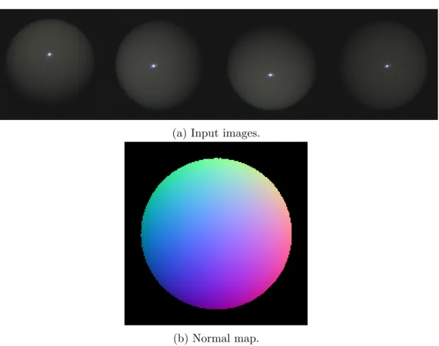
Photometric stereo is a computer vision technique for recovering surface normals of an object by observing it under different light sources. During the images acquisition the object and the camera positions are fixed, while only the light directions change as shown in figure 1.1. This approach exploits the fact that the amount of light reflected by a surface depends only on the orientation of the surface itself with respect to the light source and the observer position.
Photometric stereo has several applications in various fields. After generating the surface normals it is possible to generate the depth map and then recover the 3d model of the object that can be used in computer graphics. It can be used in industrial applications to inspect surfaces. If the surface is planar it is easy to find defects or to understand if the surface has a different shape from the one expected. It can be also useful when looking for writings that are known to be embossed. It is also used in medicine to inspect skin to assist the detection of skin lesions and illnesses such as melanoma.
1.2
WOODHAM’S ALGORITHM
Before going any further it is necessary to introduce some key concepts. Irradiance and radiance are two measures of how a surface interacts with light. In particular
(b) Normal map.
Figure 1.1: Example of photometric stereo. The RGB channels of the normal map represent respectively x, y and z axes.
the irradiance is the amount of light incident on a surface while the radiance is the amount of light emitted by a given surface in a certain direction. The reflectance is the ratio of radiance to irradiance, i.e. the fraction of light reflected on the total amount received and it depends upon the optical properties of the surface material. The reflectance model of a surface is described by a complex function called Bi-Directional Reflectance Function (BDRF). Accordingly, it is possible to measure the amount of light emitted in a certain direction given the amount of light received from the sources. Various idealized reflectance models have been defined such as the Lambertian or diffuse model, that assumes that light spreads isotropically, and the specular model, that assumes that light is reflected in only one direction.
1.2.1
HYPOTHESIS
The photometric stereo was first introduced by Robert J. Woodham in 1980[1] and it is build on the top of three assumptions:
• the surface has a Lambertian reflectance
• the camera is orthographic and has a linear radiometric response • the light rays are parallel and uniform
Enforcing the surface to have a Lambertian reflectance reduces the complex-ity of the problem, in fact the surface appears equally bright from all viewing directions. Assuming an orthographic projection, the viewing direction become constant for all object points. If the size of the object in view is small compared to the viewing distance and the focal length of the camera is big, then the perspective projection can be approximated to an orthographic projection and light rays can be considered parallel. Thus, for a fixed viewer and light source direction, the ratio of scene radiance to irradiance depends only on surface gradient. Further, suppose each object surface element receives the same incident radiance, i.e. the light rays have the same intensities, and camera has a linear response, i.e.the device produces image irradiance proportional to scene radiance. Then, the scene radiance, and hence image intensity, depends only on surface gradient.
1.2.2
THE ALGORITHM
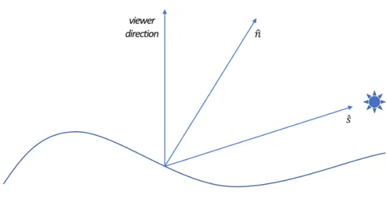
Now let’s consider a coordinate system where the viewing direction is aligned with the negative z-axis, the vector pointing the towards the viewer is thush0 0 −1
i . The surface normal vector and the vector which points in the direction of the light source can be defined respectively as: ~n = hp q −1
i
and ~s = hps qs −1
i as shown in figure 1.2.
The Lambertian reflectance model can be described using the Lambert’s cosine law by E = ρ cos(θ). Here E is the radiance, ρ is the reflectance factor and θ is the angle between the vectors ~n and ~s.
Figure 1.2: Representation of the vector defined in the Woodham’s algorithm.
If camera response is linear, then radiance coincides with the intensity of a pixel:
E = I ⇒ I = ρ cos(θ)
With a little bit of algebra it is possible to get the value of cos(θ):
~n · ~s = pps+ qqs+ 1 =
p
p2+ q2+ 1pp2
s+ qs2+ 1 cos(θ)
Then pixel intensities can be expressed as:
I = ρ(pps+ qqs+ 1) pp2+ q2+ 1pp2
s+ qs2+ 1
This is an equation with six variables, three of which are known (I, ps, qs) and
three are unknowns (ρ, p, q), so at least three images are necessary to solve the problem.
Let I = hI1 I2 I3
iT
be the column vector of intensity values recorded at a point (x, y) in each of the three images. Further let li =
h
li1 li2 li3
iT
be the unit column vectors defining the three directions of incident illumination and construct the matrix L = hl1 l2 l3
iT
. Finally let N = hN1 N2 N3
iT be the column vector corresponding to a unit surface normal at a point (x, y). Then:
I = ρLN
Provided that L is non singular, i.e. the three light direction vectors do not lie on the same plane, the solution is:
ρ =k L−1I k N = ρ−1L−1I
Considering a more general case, where more then three images are available, L is no longer square, so it is necessary to refer to the Moore-Penrose inverse:
ρ =k (LTL)−1LTI k N = ρ−1(LTL)−1LTI
It worth pointing out that in the latter case the solution can be obtained by solving the system in a least square sense.
1.2.3
LIMITATIONS
The method introduced by Woodham is simple and efficient but the three as-sumption are quite restrictive. If one of them is not met, the output cannot be considered reliable and the results are not good.
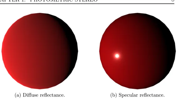
The major problem arises from the assumption of a Lambertian reflectance, as it doesn’t quite hold in the real world. Most of the real objects doesn’t exhibit a perfect diffuse reflection, common materials like plastic and metal shows specular reflections (figure 1.3) that create highly reflective points and affects negatively the results.
Another limitation comes from the need to know exactly the direction of the light sources. For this reason a light calibration process is required. This step requires effort and time, increasing the complexity and slowing down the whole
(a) Diffuse reflectance. (b) Specular reflectance.
Figure 1.3: Comparison of diffuse and specular reflectance.
photometric stereo procedure. It is also important to perform it accurately and be sure that there is no ambient lighting because it directly affects the quality of the computed surface normals and just a small error can cause the results to be bad. In addition Woodham’s algorithm can’t deal properly with complex surfaces, e.g. features like interreflections and shadows, that are not rare in real world ob-jects. Interreflections occurs when the part of illumination of the object comes from the object itself. This could happen if the object has some concavity and causes image measurements to be brighter than expected. Shadows can be classi-fied in two types: attached and cast, as shown in figure 1.4. An attached shadow occurs when the object surface curves away from the light source, causing that region to become darker. A cast shadow occurs when part of the object blocks the light from reaching the rest of the surface and cast a shadow onto itself.
All these constraints contribute to limit the range of possible application of Woodham’s algorithm, but this technique established a new field of computer vision. In fact, after the introduction of this technique by Woodham, many meth-ods has been proposed to make photometric stereo more practical relaxing some of these constraints and extending the applicability to more object shapes and materials. Furthermore in the last few years a completely new approach has been proposed using deep learning techniques and in particular convolutional neural networks, where, instead of developing complex mathematical models, a mapping
(a) Attached shadows. (b) Cast shadows.
Figure 1.4: Comparison of attached and cast shadows.
from captured images to surface normals given light directions is directly learned from examples. It is producing promising results and in the future it could com-pletely overcome current methods. Nevertheless uncalibrated photometric stereo, i.e. without the knowledge of light directions, and the handling of complex surface reflectances are still two open challenges.
DEEP LEARNING
Artificial intelligence can be described as any technique that enables computers to mimic human behaviour. Machine learning is a sub-field of artificial intelligence and it deals with algorithms that can learn and perform tasks without being ex-plicitly programmed. In particular deep learning is a machine learning method based on artificial neural networks.
What characterizes deep learning most and differentiates it from machine learn-ing is the type of data that it can process. Classic machine learnlearn-ing algorithms cannot directly handle raw data like text, images, videos or audios, and require a pre-processing step called feature extraction. The result of feature extraction is an abstract representation of the raw input data that can be used by classic machine learning algorithms to perform a task. Feature extraction can be complicated and requires detailed knowledge of the problem domain, but most of all it is time con-suming. In deep learning the neural network is able to perform this step on its own and automatically discover the representation needed. This replaces manual feature engineering and increase the performances.
Deep learning techniques can be classified into three main categories:
• supervised • unsupervised • semi-supervised
hand it can be more unpredictable and hard to manage. It is used for example to perform clustering and dimensionality reduction.
Semi-supervised learning is an hybrid of the two previous methods and com-bines a small amount of labeled data with a large amount of unlabeled data during training. The reason is that labelling data can be expensive in terms of effort and time, while unlabeled data are very cheap and, when used in conjunction with a small amount of labeled data, they can produce considerable improvement in performances.
2.1
ARTIFICIAL NEURAL NETWORKS
Artificial neural networks are inspired by the understanding of the biology of hu-man brain and their structure try to mimic the neurons and the signal transmission through the synapses.
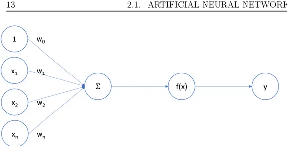
The structural building block of a neural network is an artificial neuron called perceptron. It’s behaviour is very simple: it combines inputs by means of a weighted sum plus a bias value, passes the outcome to a non-linear filter func-tion and finally outputs the result. An example of the perceptron structure can be seen in figure 2.1.
The use of a non-linear activation function is really important since it allows the network to approximate arbitrarily complex functions. If the activation functions were linear, no matter how many layer the network had, nothing better then a linear function could be computed and thus the neural network would behave like a single-leyer network (in fact the composition of two or more linear functions is
Figure 2.1: Perceptron flowchart: input weighted sum nonlinear function -output.
still a linear function). For this reason, it is a common practice to use a non-linear activation function to achieve sufficiently complex behaviours.
2.1.1
FEED FORWARD NETWORKS
A neural network can be seen as a graph, where the nodes are the perceptrons and inbound/outbound arcs are inputs/outputs of the perceptron. The simplest model is the feed forward neural network where neurons are organized into multiple layers. Neurons of one layer connect only to neurons in the immediately following layer, with no connections directed to the same or previous layers. The first layer receives the input data while the last layer produces the final result. The intermediate layers are called hidden layers, here neurons are connected to neurons in the next layer. If all neurons in each layer are connected with all neurons in the following layer, then the network is also fully-connected. A feed forward neural network is therefore a directed acyclic graph where source nodes are the input neurons and sink nodes are the output neurons.
The computational power of a feed forward neural network is defined by the Universal Approximation Theorem that states that a neural network of this kind with a single hidden layer containing a finite number of neurons can approximate any continuous real function. Thus, a simple neural network can be trained to learn various and complex functions with the right parameters, anyway, it does
• backward propagation
During the first step the input data are propagated from source nodes through the network, layer by layer. Each neuron applies his weights and his filter function, then passes the output to the following neurons until the data reach the output layer and the result is generated.
To minimize the loss function the weights of the network must be tuned prop-erly. A widely method used is the backward propagation, simply called backprop-agation. There are various algorithm that implement this method, but all rely on the same concept. The key idea is to compute the gradient of the loss function with respect to the weights of the network for each input-output example and consequently update the weights according to the gradient value trying to reach global minimum of loss function.
2.1.2
CONVOLUTIONAL NEURAL NETWORKS
Convolutional neural networks are a particular type of neural network designed for processing data that has a known grid-like topology. They are used especially for images and videos, thus very useful for computer vision tasks. In fact the behaviour and structure of this kind of neural networks are inspired to the biological processes and organization of the animal visual cortex. Convolutional neural networks take their name from convolution operator and they are defined as neural networks that use convolution in place of general matrix multiplication in at least one of their layers[2].
Each convolutional layer is composed by three stages:
• convolutional stage • detector stage • pooling stage
Figure 2.2: Common structure of a convolutional neural network.
In convolutional stage several convolutions are performed in parallel to pro-duce a set of feature maps. The convolution operation can be thought like sliding a matrix called kernel across the whole input image and performing matrix mul-tiplication at each pixel position as shown in figure 2.3. In the detector stage a non-linear function is applied for the same reason described in the previous sec-tion, i.e. to allow the network to learn more complex behaviours. In the pooling stage the pooling function replaces the output of the convolution layer at a certain location with a summary statistic of nearby outputs. It is useful because helps to make the network invariant to translations of the input. A scheme of the three stages can be seen in figure 2.2.
Convolutional neural networks have several advantages with respect to fully-connected neural networks. The convolution operation is always performed with a kernel that is much smaller with respect to the input, therefore neurons in one layer are connected only to few neurons of the following layer. Moreover each member of the kernel is used at every position of the input. Thus sparse interaction and parameters sharing both allow to reduce the memory requirement and improve
statistical and computational efficiency. Parameter sharing has also another con-sequence, equivariance to translation. This means that applying a translation to the output of the network is the same as giving the network a translated input. Last but not least, another important property is that convolutional neural net-works can have an input of any size, while fully-connected are constrained with a fixed-size input. In fact, in the latter case adding data to the input means more weights to learn while in the former case, because of the reuse of parameters, there is no need to make any change and the computation is straightforward.
2.2
TRANSFER LEARNING
2.2.1
DEFINITION
Deep neural networks are very good at learning when trained properly and can achieve performance otherwise unreachable with classic algorithms. The main drawback is that these models are extremely data-hungry and thus rely on huge amount of data to achieve their performance. Moreover they learn a very domain-specific behaviour and generally they lack the ability to generalize to conditions that are different, even slightly, from the ones encountered during training. There-fore, when performing a different task, neural networks efficiency drops and they need to be rebuilt from scratch using newly collected training data. In many real world applications, it is expensive or almost impossible to recollect the needed
training data and rebuild the model.
The ability to exploit previous acquired knowledge and overcome these issues is generally known as transfer learning. The study of transfer learning is motivated by the fact that people can intelligently exploit knowledge learned previously to solve new similar problems with less effort and better solutions. Transfer learning is the ability of a system to recognize and apply knowledge and skills learned in previous tasks to novel tasks. This technique has also other benefits. In fact adjusting an already existing model instead of creating a new one from scratch could help the model to achieve better performance and in particular speed up the training phase.
Before giving a formal definition of transfer learning, it is necessary to introduce the concepts of domain and task[3].
A domain D = {X , P (X)} consists of two components: a feature space X and a marginal probability distribution P (X), where X = {x1, ..., xn} ∈ X . Considering
a specific domain D, a task T = {Y, P (Y | X)} consists of two components: a label space Y and a conditional probability distribution P (Y | X) that can be learned from the training data, which consist of pairs {xi, yi}, where xi ∈ X and
yi ∈ Y.
Given a source domain DS and learning task TS, a target domain DT and
learning task TT, transfer learning aims to improve the learning of the conditional
probability distribution P (YT | XT) in DT using the knowledge in DS and TS,
where DS 6= DT or TS 6= TT.
Given source and target domains DS and DT where D = {X , P (X)} and
source and target tasks TS and TT where T = {Y, P (Y | X)}, 4 scenarios of
transfer learning arise. For the sake of clarity, the cases will be presented with brief examples referring to document classification, a problem where the goal is to classify a given document into several predefined categories:
• XS 6= XT → different input feature space: the documents are described in
different languages
• P (XS) 6= P (XT) → different input marginal probability distribution: the
it will be necessary to teach the neural network which is the difference between the two distributions in order to adapt and learn the new behaviour and thus perform well on target distribution.
2.2.2
FINE-TUNING
The technique used in this thesis to perform transfer learning is know as fine-tuning. Fine-tuning is a supervised approach that consists in training a neural network starting from a pre-trained model. It is very useful to speed up the training time and in particular when the dataset is too small to train a new neural network from scratch.
A common practice is to freeze some of the earlier layers, i.e. keep them fixed, and fine-tune only the last layers. This choice is motivated by the observation that earlier layers contains more generic features that should be useful for various and different tasks, while later layer becomes gradually more domain-specific. For example, considering a convolutional neural network for classification of images containing animals, the first layers will contain simple features like edge detectors and blob detectors whereas later layers will contain high-level feature that can recognize eyes and paws.
Another usual practice is to set smaller learning rate during fine-tuning of the network with respect to the one used during training of the original model. The reason is because the weights are expected to be relatively good, so they don’t have to be changed too quickly and to much. A common practice is to set the learning rate 10 times smaller than the starting one.
SETUP
3.1
HARDWARE
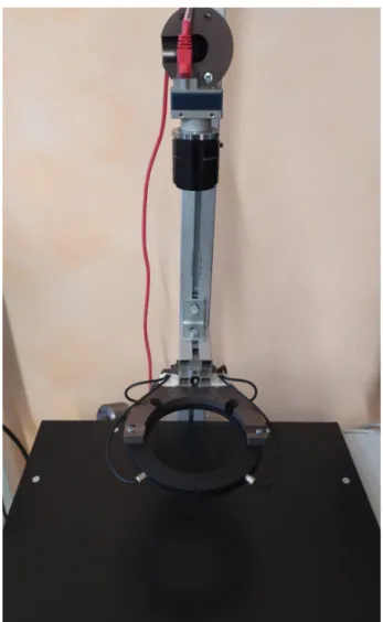
The setup for the creation of the photometric stereo dataset is composed by three elements: a camera, a light ring as light source (both showed in figure 3.1) and a controller to manage the interaction of the other two components during the images acquisition.
The camera used is monochromatic with a 1280x1024 resolution and it is equipped with a 25mm focal length optic. The light source is a 4 sectors con-trollable light ring with adjustable intensity, and it guarantees an almost uniform illumination at various distances from the plane. The controller has 4 output channels and allows to control each sector of the light ring separately and help synchronize them with the camera
The orthographic camera wasn’t available, but as explained in chapter 1, it is possible to approximate this behaviour under certain assumption. In fact the camera is placed about 50 centimeters away from the plane and the 25mm focal length lens was the higher at hand. This configuration gives a good approximation of an orthographic projection to proceed in the next photometric stereo steps.
Both lights calibration and images acquisition processes were possible thanks to the software developed by Andrea Campisi for his thesis. He realized a program that interfaces with the controller through the specific SDK and allows to easily manage lights and camera parameters and to speed up the whole process.
Figure 3.1: The setup used for the images acquisition.
3.2
LIGHTS CALIBRATION
The first step is to determine the light directions through the lights calibration. To make this phase more robust and precise, two lights calibration methods are used. Then the two outputs are merged together. In general for this lights calibration is necessary to use a reference object and take an image for each incoming light direction. Then, after extracting some kind of knowledge from images, it is possible to recover light directions.
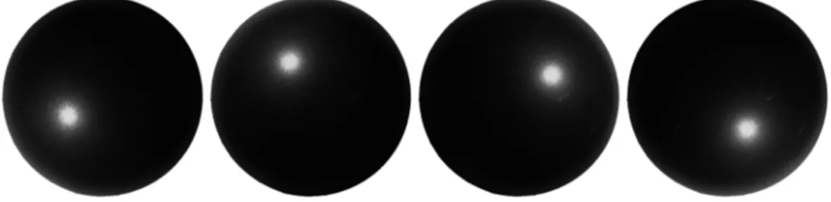
widely used technique based on the use of an highly reflective dark sphere (figure 3.2), i.e. it should ideally have a specular reflectance. To deploy this algorithm it is necessary to know the sphere radius and its position with respect to the camera, both information can be extracted directly from the taken images. Since this two parameters are known it is possible to recover the light source directions from the position of the highlights present on the surface of the sphere.
Figure 3.2: Example of images of the reference object used for the first method of light calibration.
The second method is an implemented algorithm in the computer vision soft-ware Halcon. This one is based on the use of an opaque white sphere (figure 3.3) and it is very similar to the Woodham’s algorithm. The difference is that, a part from the pixels intensity, the other known variable is surface normals instead of light directions. This is possible as it assumes the object to be a perfect sphere, so it can compute the surface normals offline, thus it recovers light directions by solving the equation that can be seen as a sort of reversed Woodham’s algorithm.
Figure 3.3: Example of images of the reference object used for the second method light calibration.
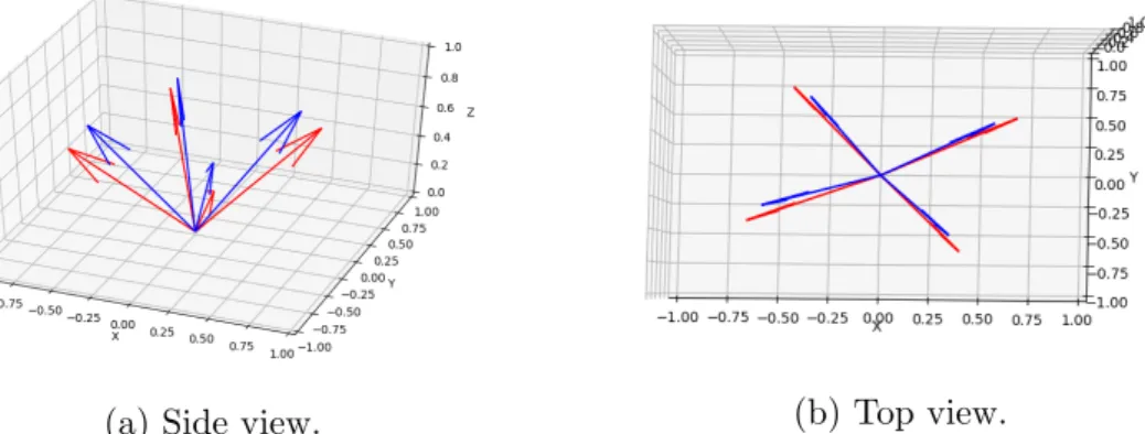
The two algorithm produce a similar but slightly different output. Using spher-ical coordinates, it is possible to express the resulting vectors with just azimuthal
(a) Side view.
Figure 3.4: Different views of the results of the 2 calibration algorithm. In blue the black sphere method, in red the white sphere method.
The azimuthal angles are always very close while regarding the polar angles, the difference is of about 10 degrees on average as shown in figure 3.4. Since it is not possible to know a priori which one is predicting correctly or similarly which one is closer to the ground-truth, for each light direction the final result is taken as the bisector of the two predicted vectors.
3.3
IMAGES ACQUISITION
To create the dataset all objects are placed below the camera, one at the time, and a single image is taken for each incoming light source. The objects selected are 13 and they are very different from each other in the shape and in the material they are made.
The surfaces range from almost planar to more complex shapes, from smooth to rough, with some objects also presenting attached and cast shadows. There is a high variety of materials, the object are made for example of plastic, metal, polystyrene and ceramic, thus the dataset has a large collection of surface re-flectances like for example diffuse, glossy and specular. All these features make the dataset very heterogeneous and will help to perform more accurate tests. Ex-amples of objects of the dataset can be seen in figures 3.5, 3.6 and 3.7.
(a) Coffee cup.
(b) Ceramic statuette.
Figure 3.5: Some of the objects in the dataset.
possible to take all images one more time but under different illumination. This process is repeated 9 times and at each iteration different light directions are used by rotating and moving up and down the light ring. Moreover, at each iteration and for all objects, the whole range of light intensities is used, in this way each object will appear both dark and bright in the dataset.
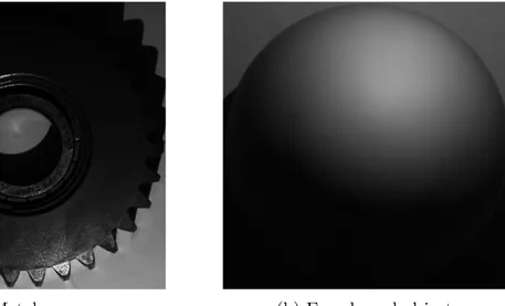
(a) Metal gear. (b) Egg shaped object.
Figure 3.6: Some of the objects in the dataset.
let-(a) Billiard ball. (b) Plastic duckie.
(c) Wrench.
Figure 3.7: Some of the objects in the dataset.
To enhance the quality of the images, several adjustment are applied to the setup, in particular to the led ring. First of all the entire setup is covered to remove as best as possible ambient lighting that can negatively affect the images quality. The only light present should be the one coming from light source. Regarding the light ring, each sector is composed by 10 led spread across an arc of about 90 degrees. In each sector all but one leds are covered to have a better approximation of parallel light rays illumination with a single point light source. Furthermore
it allows to simulate the rotation of the light ring, that actually cannot rotate, by just changing the uncovered leds. Futhermore the light ring is attached to an optical diffuser that is removed for the same reason just described above. The diffuser scatters light rays producing an unwanted behaviour as the illumination must be as much as similar to a parallel light rays beam.
PROJECT
For this thesis several paper on photometric stereo based on deep learning have been analyzed[4] [5] [6] [7]. Finally the Self-calibrating Deep Photometric Stereo
Networks[8] (SDPS-Net) has been chosen as the subject of this thesis. The reason
is that it is the most recent work in this field and can be considered as the state-of-the-art since it provides the best results among all. The thesis project follows the paper and uses python and pytorch for deep learning as well as openCV and numpy to handle the images and the input data.
4.1
SDPS-NET
4.1.1
FUNCTIONING
In this paper the author proposes an uncalibrated photometric stereo approach for non-Lambertian surfaces based on deep learning. This method is able to determine both light directions and surface normals of an object with unknown reflectance observed under unknown varying light directions. It is an important improvement compared to the previous works, since all had some biases regarding surface re-flectance or lights distribution. The key idea is to use an architecture consisting of two convolutional neural networks. The first predicts the light directions and the light intensities while the second predicts the surface normals. Splitting the problem into two sub-problems reduces the learning difficulty compared to a single network architecture by taking advantage of the intermediate supervision. It also
work (NENet), takes as input the images and the output of the first one and estimates the suface normals.
Figure 4.1: The network architecture is composed of (a) Light Calibration Network and (b) Normal Estimation Network.
The Lighting Calibration Network is a convolutional neural network with two fully connected layers at the end. The estimation of light directions and light in-tensities is modelled as a classification problem. Predicting discrete values instead of regressing them is easier and may allow the Normal Estimation Network to better tolerate small errors in the estimations.
To simplify the problem, azimuthal angle and polar angle of light directions are predicted separately, discretizing the angles in 36 classes. The light intensities are divided in 20 classes for a possible range of [0.2,2.0]. Each image is fed into a shared-weight feature extractor to extract a feature map, called local feature as it only provides information of a single image. It alone does not provide enough
knowledge, therefore all local features of the input images are aggregated into a global feature by means of a max-pooling operation. With this strategy it is possible to extract more comprehensive information from multiple observation, and additionally, max-pooling gives invariance to the number and the order of the input images. Each local feature is concatenated with the global feature and fed to a shared-weight lighting estimation sub-network to predict light directions and light intensities. Using both local and global features, the model can produce much more reliable results than using the local features alone. Furthermore, including also the object mask for each input image can improve more the accuracy of the model. The output of both light directions and light intensities are in the form of softmax probability vectors and the result is the middle value of the range with the highest probability.
The loss function adopted is multi-class cross entropy for both light directions and intensities, and the overall loss function is
LLight = λlaLla+ λleLle+ λeLe
Here Llaand Lleare the terms for azimuthal and polar angles of the light direction,
and Le is the term for light intensity. During training, all the weights λla, λle and
λe are set to 1.
The Normal Estimation Network is a fully convolutional neural network. It first normalizes the input images using the light intensities and concatenates the light directions, both predicted by the Light Calibration Network. Training the network with the discrete predictions of the previous model instead of using the ground-truth, allows to learn a more robust behavior with respect to noise in the lightings. Similarly to the Lighting Calibration Network, this network is composed of a shared-weight feature extractor followed by a max-pooling operation. Finally a normal regression sub-network predicts the normal map. The output image is already the final result itself, therefore no further operations are needed.
Given an image of size h × w, the loss function adopted is:
LN ormal = 1 hw hw X i (1 − nTi n˜i)
for every image but just the relative value of an image with respect the other ones.
4.1.3
TESTS PERFORMED AND MODEL’S LIMITS
The Self-calibrating Deep Photometric Stereo Networks is trained on a synthetic dataset. It is a common practice to use synthetic datasets in deep learning based photometric stereo because obtaining accurate ground-truth, i.e. normal maps, from real objects is difficult and time consuming and would be infeasible to create a dataset large enough for training a neural network.
The model is tested both on synthetic and real datasets. In particular, the real dataset used for evaluation is the DiLiGenT dataset[9], a benchmark created
specifically to evaluate non-lambertian and uncalibrated photometric stereo al-gorithms performance. Anyway, this dataset contains a high number of images for each object, moreover the images have high resolution and are acquired with expensive equipment using HDR technique. All these features make the dataset suitable for benchmarking, but can’t represent a real-world scenario. In fact, in real applications, usually it is not possible to achieve this level of quality, but the greater limitation comes from the number of different lights that can be calibrated, that is usually small.
For this reason various tests are performed to understand if the Self-calibrating Deep Photometric Stereo Networks is capable of performing well also on real-world scenarios. The tests will also help to figure out the best configuration for the camera and the light source that will eventually led to the configuration described in chapter 3.
The tests will be presented in a chronological order, explaining the reasons behind the choices and the observations for each test.
The first tests are performed on images acquired by varying light directions and intensities, exposure time and aperture of the camera in order to get different calibrations and both bright and dark images. The predicted surface normals are really bad, even if a ground-truth isn’t available, it is clear that the predictions are completely wrong. By checking the intermediate results, i.e. light directions and intensities, and comparing them with the ground-truth, it turns out that they are wrong too.
The first idea is that a likely reason of the errors could be the low number of images used for each object, 4 images instead of the 32 used for training the model and the 96 used in the DiLiGenT benchmark. Therefore in the next test a little subset of images for each object of the DiLiGenT dataset is used. The results show that, after feeding the network with a low number of images, e.g. 4, 8 and 16, all the predictions are good anyway and the error is very little compared to the one of the thesis dataset. To better understand the relationship between the errors and the number of images in input, images from different calibrations are merged to get more than 4 images, e.g. 8 or 12 images per object. No improvement are observed, nor in the prediction of light directions and intensities neither in the surface normals. These results demonstrate that the number of images isn’t the cause of the bad performance.
The next idea is that another possible reason of the errors can be the type of illumination. Two other types of illuminator are tested in place of the light ring. Unfortunately it isn’t possible to calibrate these kind of lights, therefore only the normal maps results can be checked. Even using a larger number of images, e.g. from 10 to 20 images per object, the normal maps are still bad and there is no improvement with respect to the light ring. These results proved that even the type of illumination isn’t the source of the problems.
The turning point comes when the setup is covered to remove as much as possible the ambient light. Previously, to remove ambient light, an image with no light source turned on was taken and then subtracted to the other images (this procedure is still used even with the setup covered as it provides a little improvement). The error of the estimated light directions decrease significantly
First the Normal Estimation Network is fed with both ground-truth and es-timated light intensities, that are quite different, but the results are almost the same. Thus the light intensities values do to not influence the normal maps results. For the second test the object for which the predicted light directions are bad are considered. This time the network is fed with both ground-truth and estimated light directions. The results changes slightly, sometimes for better, sometimes for worse, but never improves significantly. Therefore it seems that the objects have some intrinsic features that make the network to perform badly.
Now, since the results of estimated light directions are promising, the next tests will be focused on Lighting Calibration Network only, since it is quite useless to work on Normal Estimation Network until the light prediction are not satisfactory. These tests are performed after applying some adjustements to the setup as described in the previous chapter. First the light diffuser is removed from the light ring, then all but one led of each sector of the light ring are covered, finally both expedients are used. These new setups, and the last in particular, show slight improvements, but nothing really relevant.
Overall the tests showed the best setup to acquire the images but also the model limitations. Changes in the setup improved the performance, but the re-sults are still far from satisfactory. The Self-calibrating Deep Photometric Stereo Networks struggles to predict well the light directions, in particular the polar an-gle, and in general the normal maps are estimated badly. Furthermore the network performance seems to be strictly linked to some, not well understood, features of the objects. Some perform well no matter of the setup used, and the same goes for the objects that perform badly.
Since the adjustments to the setup are not sufficient to achieve a decent perfor-mance, the next steps will be focused on transfer learning and how to adjust the network to overcome the current limitations and perform well on all the objects.
4.2
FINE-TUNING LCNet
4.2.1
DATASET
Before fine-tuning the network it is necessary to prepare the input images alongside with the ground-truth necessary to compute the loss function, i.e. light directions and light intensities.
After acquiring the images for an object, one more image is acquired with no lights turned on. Being the setup covered the residual ambient light in the scene is very low and the ambient image is almost completely dark. Nevertheless it is subtracted to the other images since experimental results showed that this operation can improve the quality of the image.
For each image in input, the Lighting Calibration Network needs light direction and light intensity. The light directions are obtained with two light calibrations methods as explained in chapter 3. The ground-truth direction is chosen as the bisector of the resulting vectors of the two methods. The light intensities are simply taken from the settings of the light ring. In fact there is a percentage value that allows to choose the intensity of light emitted by the leds. Since the network need the intensities to be in the range [0.2, 2], the values can be trivially converted from the range [0, 100] to the new range.
Then, it is necessary to calculate the mask of the objects. It is not mandatory but it can improve the performance of the network. Since the objects in the dataset are very heterogeneous, it is not trivial to find a straightforward method to compute all the masks. For example, image thresholding with Otsu’s algorithm doesn’t work well as it fails to compute straight edges on the objects border, moreover the mask can contain some holes. Even Canny edge detector is quite useless since it is necessary to continuously tune the parameters, e.g. there are images both bright and dark. Furthermore the result only contains edges and thus another step is necessary to compute the final mask. For this reasons to compute
contain only the background. Thus it is first necessary to extract contour points of the object, then to find the minimum enclosing rectangle that has the same orien-tation of the image. This is done by means of OpenCV functionsfindcontours() andboundingrect(). The findcontours() function takes as input a binary image and returns a list of contour points, therefore the contours are extracted from the mask image. The boundingrect() function takes as input a list of points, in this case the computed contour points, and returns the coordinates of the vertices of the minimum enclosing rectangle. With this information the images and the mask image can be trivially cropped around the object.
Before feeding the images to the network a data augmentation step is imple-mented. Data augmentation is a technique that enhance the size and the quality of training dataset. It consists in a series of transformations applied to the training images, examples are rotation, flipping, cropping, noise injection and color space transformation. This technique is particularly useful when the training dataset is relatively small, but it can always be used to avoid overfitting and to improve the network generalization ability. For the training of Lighting Calibration Network only cropping is adopted. The reason is that each image is associated to a light direction, thus geometric transformations would affect this correspondence, e.g. if the image is rotated, then the corresponding light direction would no longer be correct. Noise injection increases the training time without improving in the accuracy, thus it is discarded.
The last layers of the Lighting Calibration Network are fully connected and therefore it is required a fixed-size input. Thus the last operation performed is a resize of the images to a size of 128x128.
In supervised learning it is a common practice to split the dataset in three distinct sets:
• training set • validation set • test set
The training set is a set of paired data, i.e. input and expected output, used for training the model and thus to adjust the network’s weights.
The validation set is a set of paired data used to evaluate the performance of the trained model and tune it consequently. For example, it is used to verify that any increase in accuracy over the training set actually corresponds to an increase in accuracy over the validation set. If the accuracy over the validation set decreases it means that the model is overfitting the data. In general it is useful to tune the model hyperparameters, i.e. parameters whose values are set before the training begins. In fact each iterations of training and validation can tell how changes in the model reflects in its accuracy. In other words, the training set allows to find the best weights and the validation allows to find the best hyperparameters. After this two steps, the best model is finally tested on the test set.
The test set contains paired data and it is used to evaluate the performance of the final model on real-world scenarios. After assessing the final model on the test set, the model must not be tuned any further.
To guarantee reliable results it is fundamental that all the three sets contain different data, i.e. the sets must be disjoint.
To validate the Lighting Calibration Network cross-validation is employed. Cross-validation is a model validation technique that help to reduce the variability when splitting the dataset in training set and validation set. Generally a multi-ple rounds of validation are executed using different partitions and the results are combined to better estimate the model performance. In particolar, the method adopted is k-fold cross-validation. It is a non-exhaustive method since it does not compute all ways of splitting the dataset. K-fold cross-validation splits the dataset in k samples, one is used as the validation set while the other k − 1 are used as the training set. This process is repeated k times, with each of the k samples being
Hence the same object uses different calibrations when is in one of the three set.
4.2.2
FINE-TUNING
The description of the project will approximately follow the code execution and only the salient sections will be presented.
To find which are the best hyperparameters of the model, a grid search is employed. It means that all the combinations of hyperparameters are tested but, since the training doesn’t take too much time, this doesn’t represent a limitation (code snippet 4.1). The hyperparameters used are four:
• learning rate • training batch size
• L2 regularization coefficient • layers to freeze
Code Snippet 4.1: Grid search for hyperparameters tuning.
1 for i, (lr, lt, bs, l2) in enumerate(itertools.product (lr_values,
lt_values, bs_values, l2_values)):
,→
2 learning_rate = lr 3 layers_to_train = lt
4 training_batch_size = bs 5 l2_regularization = l2 6
7 # training
The learning rate is a parameter that represents how much the weights are changed at each backpropagation step. Metaphorically speaking, it represents the speed at which the neural network learns. The value of learning rate is critical for the success of the training. With small learning rate the loss function converges slowly and gets stuck in false local minimum. With large learning rates the loss function becomes unstable and diverge. For this reason, it is a common practice to use an adaptive learning rate that decreases during training.
The batch size defines the number of samples that will be propagated through the network at each iterations. Using higher batch size requires more memory but makes the training faster since the backpropagation step is executed fewer times. Increasing the batch size too much causes the degradation of the generalization ability of the network. A too small batch size has disadvantages too. The smaller the batch size the less accurate the estimation of the gradient will be since there is an higher variance in the input. In general, this is an unwanted behaviour, but sometimes can be useful to avoid overfitting. Therefore it is necessary to find a good compromise in the batch size get a stable training to allow the network to generalize well.
Regularization is a technique to improve the network’s generalization ability and to prevent overfitting. One of the simplest and most common kind of regu-larization techniques is the L2 reguregu-larization that forces the weights of the neural network to become smaller. This is done by adding a parameter to the loss func-tion λ k w k22, where w is the vector containing all the network’s weights and λ is a coefficient that represents how much the regularization influences the loss function. In this way the network is encouraged to learn simpler functions. In-tuitively, in the feature space, only directions along which the weights contribute more to minimize the loss function are not changed. In directions that contribute less, movement in these directions will not significantly increase the gradient and thus, weights corresponding to useless directions, are decreased. Another simple
parameterrequires grad=False for each weight in the layers to freeze as shown in code snippet 4.2. The configurations for layers freezing are three: train the whole network, train only the second half of the network, i.e. after the max-pooling, and train only the last fully connected layers.
Code Snippet 4.2: Layers freezing in Light Calibration Network, here layers to train is the hyperparameter.
1 if layers_to_train == 'fully_connected':
2 for param in model.featExtractor.parameters(): 3 param.requires_grad = False
4 for param in model.classifier.conv1.parameters(): 5 param.requires_grad = False
6 for param in model.classifier.conv2.parameters(): 7 param.requires_grad = False
8 for param in model.classifier.conv3.parameters(): 9 param.requires_grad = False
10 for param in model.classifier.conv4.parameters(): 11 param.requires_grad = False
12
13 elif layers_to_train == 'second_half':
14 for param in model.featExtractor.parameters(): 15 param.requires_grad = False
17 elif layers_to_train == 'all': 18 # no layers to freeze 19 pass
Since a new model is fine-tuned for each iteration of the cross-validation, the model is copied each time to not modify the original one and avoid loading it again from disk. The dataset is loaded each time since the training set and the validation set are different at each iteration. Before fine-tuning is also necessary to set the criterion and the optimizer. The criterion is the implementation of the loss function. Given the network’s output and the ground-truth, it returns the error. The loss function used is the same as the pre-trained model, a multi-class entropy for both light directions and light intensities. The optimizer represents the optimization algorithm used to perform backpropagation. The adopted optimizer is the widely used Adam. It is an iterative method where the learning rate is adapted for each parameter. The learning rate scheduler allow to set an adaptive learning rate, in particular the learning rate is halved every 5 epochs. An example of model configuration can be seen in code snippet 4.3.
Code Snippet 4.3: Model configuration.
1 def configure_model(model):
2 modelcopy = copy.deepcopy(model)
3 parameters_to_update = [param for param in
modelcopy.parameters() if param.requires_grad]
,→ 4
5 crit = criterion.Stage1Criterion(cuda)
6 optimizer = torch.optim.Adam(parameters_to_update,
learning_rate, weight_decay=l2_regularization)
,→
7 scheduler = torch.optim.lr_scheduler.MultiStepLR(optimizer,
milestones=[5, 10, 15], gamma=0.5)
,→ 8
4.3
FINE-TUNING NENet
4.3.1
DATASET
The objects images and the corresponding mask as well as the light directions and the light intensities are obtained in the same way described for Lighting Calibra-tion Network. The images are normalized using the light intensities and then are concatenated to the light directions. This will be the input of the network. To fine-tune the Normal Estimation Network is also necessary the normal map, i.e. the ground-truth necessary to calculate the loss function.
Since it is not possible to have the real ground-truth, a method to overcome this problem is to calculate the normal maps using different algorithms[11] [12] [13] [14] [15] and average the results, i.e. for each pixel the final result is the bisector of the vectors computed by the algorithms (example in image 4.2). Then pixels will be considered differently with respect to the discordance between the algorithms, i.e. if the output of the algorithms for a certain pixel is similar, than the pixel will have more importance in the loss function. This method will be explained exhaustively in the next section during the description of the loss function.
The normal map is calculated using 4 different algorithms: 2 different imple-mentations of Woodham’s algorithm that produce two slightly different results, a lambertian photometric stereo algorithm based on sparse regression with L1 residual minimization and a semi-calibrated photometric stereo algorithm based on alternating minimization. Other algorithms are tested but since they usually
produce clearly bad results, they can’t be considered reliable and therefore em-ployed. The reason is probably that they require an higher number of images per object compared to the 4 images available in the dataset.
(a) Algorithm 1 output. (b) Algorithm 2 output.
(c) Algorithm 3 output. (d) Algorithm 4 output.
(e) Average of all the 4 output.
Figure 4.2: Example of the output of the employed algorithms and the average used as ground-truth.
The algorithms employed sometimes fail to compute the surface normal in some pixel. Since the ground-truth is the mean of these results, if an algorithm fails to compute the surface normal for a certain pixel, the ground-truth for that
normals = [x / 255 * 2 - 1 for x in normals]
4 norm = np.linalg.norm(normals, axis=3) + 1e-8 5 normals = normals / norm[:,:,:,np.newaxis] 6
7 # mask application
8 mask = cv2.imread(os.path.join(folder, mask_name),
cv2.IMREAD_GRAYSCALE) / 255
,→
9 normals = np.array([normal * mask[:,:,np.newaxis] for normal in
normals])
,→ 10
11 # elimination of pixels where the normal is not present
12 normals = np.where(normals == (127/255*2-1,127/255*2-1,127/255*2-1),
(0,0,0), normals)
,→
13 no_normal = np.where((normals == (0,0,0)).all(axis=3),False,True) 14 bisectors = np.sum(normals, axis=0,
where=np.repeat(no_normal[:,:,:,np.newaxis], 3, axis=3))
,→ 15
16 norm = np.linalg.norm(bisectors, axis=2) + 1e-8 17 bisectors = bisectors / norm[:,:,np.newaxis]
Some of the algorithms are quite slow, therefore, before computing the normal maps, the images are resized by halving both height and width to speed up the computation. This operation should not affect the training too much, since the network will be fed with crops of the resized images.
A data augmentation step is applied also during this training. The images are cropped with patches of size 128x128. This size is chosen since the original model is trained with 128x128 images, therefore it seems reasonable to use input of the same size. Some of the images need to be padded because, after the resize, some have a side lower than 128.
The network require the image sides to be a multiple of 4. During training is not a problem, since 128 is multiple of 4, but during validation, when the images are fed without changes, they need to be padded.
In the dataset there are images of 13 objects, 10 are used for training and validation, 3 are used for test. During training k-fold cross-validation is employed with k = 10, in this way one single object is validated at each iteration. The nine calibrations are always used, so the same object uses all the calibrations regardless of the set in which it is.
4.3.2
FINE-TUNING
The code for fine-tuning Normal Estimation Network is similar to the code de-scribed in the previous section for Light Calibration Network. Therefore part of the code is reused and only the main differences will be described.
The four hyperparameters used are the same as well as the optimizer for back-propagation, i.e. Adam, and the learning rate scheduler, i.e. learning rate halved every 5 epochs.
The configuration for layers freezing are only two: train the whole network and train only the second half of the network, i.e. after the max-pooling. The model is fine-tuned in the same way, cross-validation to assess the accuracy and final training to generate the final model. The number of epochs used is 30 as the network converges a little bit slower compared to the Light Calibration Network.
The most important change is about the loss function. As hinted in the previous section, the loss function is the same used for the pre-trained model but each pixel is weighted differently with respect to the discordance of the algorithms employed for the generation of the ground-truth.
The discordance is a value that intuitively represents how much some vectors are similar, i.e. they point in the same direction. For each pixel, after obtaining
not present
4 weights=np.where((normals == (0,0,0)).all(axis=3),0,1) 5 discordance = ma.average(angles, axis=0, weights=weights) 6
7 discordance[discordance.mask] = 0 8 discordance[˜no_normal[0]] = np.pi 9 discordance = np.array(discordance)
The elimination of the pixels in code snippet 4.5 is necessary as hinted in the previous section. Sometimes an algorithm can fail to produce the output for some pixels. For these pixels there is one or more less surface normal and therefore it should be taken into account during the computation of the average.
Figure 4.3: Example of discordance matrix. A black pixel means that the discor-dance is 0.
If the discordance is 0, it means that the vectors are identical. The higher it is, the more dissimilar the vectors are. The result is a matrix of the same size of the images, where each cell contains the discordance of the corresponding pixel. An example can be seen in 4.3. Since the vectors lie on an hemisphere, the maximum angle between two vectors, and so also the discordance, is π. To remove bad pixels, i.e. pixel with a high discordance, the discordance values can be clipped to a certain threshold, e.g. π2 or π6. The values are then normalized in the range [0, 1] and a weight function is employed to convert the values into weights for the loss function.
Figure 4.4: On the x axis there is the discordance, on the y axis there is the corresponding loss function weight. In red the linear function, in blue the cubic function and in green the cosine function.
The weight for each pixel is inversely proportional to the discordance, so that, if the discordance is 0, the pixel weight will be 1. Several function to convert the discordance to weights are tested: linear, cubic and cosine.
The cubic function only penalizes pixels with a high discordance whereas the cosine gives more importance to pixels with a small discordance while it also pe-nalizes the pixels with a high discordance. All the three functions can be seen in figure 4.4.
RESULTS
5.1
RESULTS FINE-TUNING LCNet
The model with the highest accuracy is found by fine-tuning the Lighting Calibra-tion Network with the following hyperparameters:
• learning rate: 0.00005 • training batch size: 8
• L2 regularization coefficient: 0.1
• layers to train: second half of the network
The learning rate of 0.00005 is a tenth of the one used for the pre-trained model. It is a common practice to set the learning to a tenth of the original one and also in this case works very well. The training batch size of 8 is a fourth of the original value used for the pre-trained model. Anyway this value seems to not influence the training too much since the results are quite good also with other values of batch size. The L2 regularization improve a little bit the accuracy of the final model. All coefficient values lower than 1 give a little improvement, whereas biggers coefficient worsen the accuracy. The first layers are freezed, thus only the second half of the network, i.e. after the max-pooling operation, is fine-tuned. The reason is probably that the first layers already contain features that work well on the training dataset. The accuracy of the final model is a bit worse when the
• light directions estimation error: – original model: 34.06 – fine-tuned model: 10.87 • light intensities estimation error:
– original model: 0.24 – fine-tuned model: 0.09
The error in the estimation of the light directions goes from 34.06 to 10.87, with an improvement of 23.19 degrees. The error in the estimation of the light intensities is decreased of 0.15. The predictions of the model improved, the new model has now an average error that is one third with respect to the original one.
5.2
RESULTS FINE-TUNING NENet
The model with the highest accuracy is found by fine-tuning the Normal Estima-tion Network with the following hyperparameters:
• learning rate: 0.0005 • training batch size: 4
• L2 regularization coefficient: 0.00001 • layers to train: the whole network
The learning rate of 0.0005 is the same used for the pre-trained model. Prob-ably the network’s weights need more refinements with respect to the Lighting Calibration Network where the learning rate used was lower. The training batch size of 4 is a fourth of the original value used for the pre-trained model, and also this time this value doesn’t influence the training too much. The L2 regularization improve the accuracy of the model just a little. The coefficient is very small and increasing it leads to the deterioration of the accuracy. With a coefficient greater or equal to 0.1 the results are completely wrong. No layers are freezed, therefore the fine-tuning is performed on the whole network. Conversely training only the second half of the network always deteriorate the results.
The choice of the object to put in the test set follows the same reasoning described in the previous section. This time the three objects are: the egg shaped object, the coffee cup and the box and .
Since the truth used to train the model actually is not a real ground-truth but it is the average of the output of several algorithms, there aren’t quanti-tative results. Of course numeric quantities, e.g. the accuracy, are used to assess which is the best model, but they can only tell which is the best model among all but not how well the model is performing exactly. For this reason the results are only qualitative.
(a) Original model. (b) Fine-tuned model.
(a) Original model. (b) Fine-tuned model.
Figure 5.2: Egg shaped object normal maps output example 2.
The resulting images of the fine-tuned model are compared with the results of the pre-trained model. Despite the images can be compared only qualitatively, it is easy to see that the fine-tuning improved the performance of the model.
The original normal maps in figure 5.1 and 5.2 are completely wrong. Only in the middle of the object there are some traces of reasonable pixels. Even if the final normal maps are not excellent, they show big improvements from all points of view.
(a) Original model. (b) Fine-tuned model.
Figure 5.3: Coffee cup normal maps output example 1.
(a) Original model. (b) Fine-tuned model.
Figure 5.4: Coffee cup normal maps output example 2.
of the object has some writings and the vertical surfaces have patches with strange colors. In the final normals maps the writings are removed almost completely and the other surfaces have a more uniform color.
(a) Original model. (b) Fine-tuned model.
Figure 5.5: Box normal maps output example 1.
The original normal maps in figure 5.5 and 5.6 show many artifacts. In partic-ular writings should not appear in the normal map as well as the lines since they are both printed. The final normal maps have a more uniform color, as it should
(b) Fine-tuned model.
Figure 5.6: Box normal maps output example 2.
be, since the object is planar and all the artifacts are removed almost completely. Moreover the braille signs are more clear.
As already mentioned, several function are employed to convert the discordance to weights, i.e. linear, cubic and cosine. The resulting normal maps are almost identical to each other. Also setting different thresholds like π
2, π
6 or even using
no threshold doesn’t improve or worsen the resulting normal maps. Therefore the most important thing for a good training is the quality of the ground-truth. Other techniques like loss weighing and concordance clipping, that at first seemed good ideas to improve the results, are shown to be quite useless.
Regarding the execution time, the deep learning model completely outperforms all classic photometric stereo algorithm employed. In part is due to the fact the model executes on GPU, but the model is certainly way more fast. The compu-tation time depends on the input image size and on the number of input images, but on average the model takes less than 0.005 seconds per object to generate the normal maps. A part from the Woodham’s algorithm that takes about 0.050