diogene alessandro dei tos
M a r c h i o e l o g o t i p o d e f i n i t i v o a c o l o r i s e n z a f o n d o .
Dynamical substitutes of Larangian points and quasi-periodic orbits about them Master of Science
Department of Aerospace Science and Technology Space Engineering
Politecnico di Milano July 2014
quasi-periodic orbits about them, Master of Science supervisor: Dr. Francesco Topputo location: Milano time frame: July 2014
— Lilo & Stitch —
Dedicated to the memory of my grandfather Gelindo, who taught me that being a man sometimes means give up. Shall his memory never fade from
The restricted three-body problem (RTBP) is the ideal model to design unique solutions, ranging from Lagrange point orbits to low energy transfers. These orbits embed the effect of two gravitational attractions in a natural way, and therefore they are more accurate than the conics, solutions of the classic two-body problem. However, when three-two-body orbits are reproduced in the real solar system model, large errors are found. That is, as the three-body orbits are defined in the regions of phase space where the sensitivity is high, the additional terms of the real solar system model produce large effects along the orbits.
The core of this thesis is to present an automatic algorithm for the correc-tion of orbits in the real solar system. The differential equacorrec-tions governing the dynamics of a massless particle are written as perturbation of the RTBP in a nonuniformly rotating and pulsating frame by using a Lagrangian formalism. The refinement is carried out by means of a multiple shooting technique, and the problem is solved for a finite set of variables. The generality of the algo-rithm lies in the possibility of handling both constrained and unconstrained boundary conditions. In the latter case, the problem is solved by minimising a certain performance index. Once the problem is stated, the gradient of the objective function, as well as the Jacobian of the constraints are computed and assembled in an automatic fashion.
Results are given for the dynamical substitutes of the collinear points of sev-eral three-body systems. Periodic and quasi-periodic orbits in the framework of the RTBP (e.g., halo orbits) are refined in the full gravitational solar system model by means of the proposed method.
The trajectory-refinement algorithm has been implemented with the idea of being versatile. With minor adjustments to the code backbone it can be applied to a large variety of practical astrodynamics problems, from stable orbits to optimised propelled trajectories and orbits that exploit the intrinsic dynamics of the solar system.
Il problema ristretto dei tre corpi (RTBP) è il modello ideale per calcolare soluzioni uniche, che vanno da orbite nell’intorno dei punti Lagrangiani ai trasferimenti a basso consumo energetico. Queste traiettorie incorporano l’ef-fetto di due attrattori gravitazionali in modo naturale, e si prestano dunque ad uno studio più accurato rispetto alle coniche, soluzioni del classico problema di Keplero. Tuttavia, quando le orbite dei tre corpi sono riprodotte nel modello reale del sistema solare, si trovano grandi errori. In particolar modo, quando queste orbite sono definite nelle regioni dello spazio delle fasi in cui la sensi-bilità è elevata, le perturbazioni dovute ad altri corpi producono grandi effetti lungo le orbite.
Il fulcro di questo lavoro di tesi giace nello sviluppo di un algoritmo auto-matico per la correzione delle orbite al modello gravitazionale completo che descrive il sistema solare. Le equazioni differenziali che regolano la dinamica di una particella priva di massa sono scritte come perturbazione del RTBP in un sistema non uniformemente rotante e pulsante, utilizzando un formalismo Lagrangiano. La procedura di affinamento avviene mediante una tecnica di multiple shooting, e il problema è risolto per un insieme finito di variabili. La generalità dell’algoritmo consiste nella possibilità di gestire condizioni al contorno sia vincolate che non vincolate. In quest’ultimo caso, il problema è risolto tramite minimizzazione di un determinato indice. Formulato il prob-lema, il gradiente della funzione obiettivo e il Jacobiano dei vincoli vengono calcolati e assemblati in modo automatico.
Vengono forniti i risultati per i sostituti dinamici dei punti collineari di di-versi sistemi a tre corpi. Orbite periodiche e quasi-periodiche nel quadro del RTBP (ad esempio orbite halo) sono affinate nel modello completo a n corpi mediante il metodo proposto.
L’algoritmo di affinamento della traiettoria è stato implementato con l’idea di essere versatile. Con aggiustamenti minori al codice, esso può essere appli-cato ad una grande varietà di problemi pratici dell’Astrodinamica: da orbite stabili ad ottimizzazione di traiettorie propulse e orbite che sfruttano le di-namiche intrinseche del sistema solare.
— Ralph Waldo Emerson —
A C K N O W L E D G M E N T S
I would like to thank professors Franco Bernelli Zazzera and Michèle Lavagna for their availability and readiness in answering my questions, both directly related to the thesis and concerning my future academic career. I withal appreciated the help of Dr. Luigi Mingotti.
I am grateful to my supervisor, Dr. Francesco Topputo, not only for his scientific support during the whole study period, but also for his human atti-tude towards me. He guided and followed me in this last part of my Master of Science.
Acknowledgements to my friends, which were there even if I was not. In particular to Marf, who taught me the intricacy of moralism and maybe brought me nearer to the engineering world; to Monai, fellow in misfortune; and to Vittorio Veneto’s old dudes.
A special thank goes to ‘polletti’ Patrik, Sergio and Paolo, companions of adventure and shenanigans in ‘Middle Earth’, with whom I share the best, most hilarious and most difficult memories of my life.
Un immenso ringraziamento alla mia famiglia, mamma, papà, Mattia, Raffaele, Stefano, nonna Gianna e nonni paterni; che mi è stata vicino anche nella lontananza, e mi ha aiutato imperterrita in tutti questi anni.
Diogene Alessandro Dei Tos
1 introduction 1
1.1 Historical legacy 1
1.2 Motivation and goals 3
1.3 State of the art 5
1.4 Organisation of the work 8
2 dynamics models 9
2.1 The problem of n bodies 9
2.2 The Kepler problem 12
2.2.1 Conservation of energy 13
2.2.2 Conservation of angular momentum 14
2.2.3 The trajectory 14
2.2.4 Kepler’s laws 15
2.2.5 Orbit in three dimensions 16
2.3 The restricted three-body problem 19
2.3.1 Equations in the synodic frame 21
2.3.2 Lagrangian points 25
2.3.3 Motion near the equilibrium points 30
3 equations of motion in the roto-pulsating frame 41
3.1 Change of coordinates and Lagrangian formulation 42
3.2 Coefficients for the equations of motion 52
3.3 Fourier analysis of the motion equations’ coefficients 54
4 integration and validation 65
4.1 Integration scheme 65
4.1.1 Multi-step methods 67
4.1.2 Runge-Kutta methods 70
4.2 The JPL ephemeris model 71
4.2.1 Julian days count 75
4.3 Validation of the dynamical problem integration 78
4.3.1 Solar system barycentric integration 85
4.3.2 Roto-pulsating integration 88
4.3.3 Double-way validation 95
5 method and results 99
5.1 Two-point boundary value problem 99
5.1.1 The simple shooting technique 100
5.1.2 The multiple shooting method 103
5.2 The trajectory refinement algorithm 107
5.2.1 The modified multiple shooting 110
5.3 Dynamical substitutes of libration points 113
5.4 Quasi-periodic orbits refinement 119
5.4.1 The halo family 119
5.4.2 The planar Lyapunov family 121
6 final remarks 125
6.1 Conclusions 125
6.2 Prospective work 126
a rotation matrices properites 131
a.1 Properties of CT˙C 131
a.2 Properties of CT¨C 132
b fourier analysis 135
b.1 The Fourier integral: a continuous representation 135
b.2 The Fourier integral: a discrete representation 140
b.3 A refined Fourier analysis 144
Figure 2.1 Geometry of the n-body problem in an inertial reference
frame, XYZ 10
Figure 2.2 Geometry of the two-body problem in an inertial
refer-ence frame, XYZ, and relative frame, xyz 12
Figure 2.3 Elliptical orbit and its perifocal frame in the Kepler
prob-lem 15
Figure 2.4 Geocentric equatorial and perifocal frame references with
orbital parameters and Euler angles 17
Figure 2.5 Sequence of three rotations transforming I, J, K into ˆe, ˆq, ˆh.
The ‘eye’ viewing down an axis sees the illustrated ro-tation about that axis. This image is courtesy of Curtis
[11] 18
Figure 2.6 Geometry of the three-body problem in an inertial
ref-erence frame, XYZ, centred at the primaries
barycen-ter 20
Figure 2.7 Synodic reference frame for the CRTBP 23
Figure 2.8 Quintic polynomial for the evaluation of the collinear
libration points, f(x, 0, 0) 27
Figure 2.9 Color-gradient visualisation of the potential function ⌦,
for z = 0 28
Figure 2.10 Contour map of J = 2⌦, and zero-velocity curves for
µ= 0.12 at several interesting discrete values of the
Ja-cobi constant, C 29
Figure 2.11 Parameter c2 36
Figure 2.12 Planar Lyapunov orbits family for the Earth-Moon
sys-tem around the first (left) and second (right) Lagrangian
point 38
Figure 2.13 Halo orbits family around the first collinear point L1 of
the Sun-Jupiter gravitational system 39
Figure 3.1 Transformation geometry of the three-body problem in
an inertial reference frame, XYZ 42
Figure 3.2 Norm of Fourier transform of the motion equation (bi, i =
1, . . . , 6) coefficients for the Earth-Moon case 56
Figure 3.3 Norm of Fourier transform of the motion equation (bi, i =
7, . . . , 13 excluding b9) coefficients for the Earth-Moon
case 56
Figure 3.4 Norm of Fourier transform of the motion equation
co-efficients b9 for the Earth-Moon case 57
Figure 3.5 Norm of Fourier transform of the motion equation (bi, i =
1, . . . , 6, 13 excluding b3) coefficients for the Sun-Earth
case 58
Figure 3.6 Norm of Fourier transform of the motion equation (bi, i =
7, . . . , 12) coefficients for the Sun-Earth case 58
Figure 3.7 Norm of Fourier transform of the motion equation
co-efficients b3 for the Sun-Earth case 59
Figure 3.8 Norm of Fourier transform of the motion equation (bi, i =
1, . . . , 6) coefficients for the Sun-Jupiter case 60
Figure 3.9 Norm of Fourier transform of the motion equation (bi, i =
7, . . . , 13 excluding b8) coefficients for the Sun-Jupiter
case 60
Figure 3.10 Norm of Fourier transform of the motion equation
co-efficients b8 for the Sun-Jupiter case 61
Figure 3.11 Norm of Fourier transform of the x components of the
Sun (bottom) and Mercury (top). The positions are ex-pressed in Kilometres and are written in the inertial
frame of reference, centred at SSB 62
Figure 4.1 x-y projection of orbital trajectories of different small
objects, centred at Earth 79
Figure 4.2 Trajectory of the Jupiter trojan Achilles, Sun-Jupiter
roto-pulsating frame 83
Figure 4.3 Error trend for Aten, class of the near-Earth asteroids
Aten (Short period: 27 years). SSB integration. 85
Figure 4.4 Error trend for Quetzalcoatl, class of the Amor (Short
period: 27 years). SSB integration. 86
Figure 4.5 Error trend for Juno, class of the Main-belt asteroids
(Long period: 428 years). SSB integration. 86
Figure 4.6 x-y projection of orbital trajectories of different small
objects in the Jupiter (top figures) and in the
Sun-Earth synodic frame (bottom figures) 88
Figure 4.7 Error trend for Icarus, class of the Apollo. Sun-Jupiter
synodic frame 89
Figure 4.8 Error trend for Aneas, class of the Jupiter trojan.
Sun-Jupiter synodic frame 90
Figure 4.9 Error trend for Atira, class of the Atira. Sun-Earth
syn-odic frame 91
Figure 4.10 Error trend for Brucia, class of the Mars-crossers.
Sun-Earth synodic frame 92
Figure 4.11 Error trend for Hidalgo, class of the Centaurs. Sun-Earth
synodic frame 92
Figure 4.12 Error trend for Deimos, natural satellite of Mars.
Figure 4.13 Double-way validation scheme 95
Figure 5.1 Example of a simple shooting 103
Figure 5.2 Multiple shooting strategy and defects vector 104
Figure 5.3 Solution of a Lambert problem trajectory with the
mul-tiple shooting method 106
Figure 5.4 Iterations of the multiple shooting method for the
com-ponent x of the Lambert problem trajectory 107
Figure 5.5 Flux diagram of the iterative algorithm for orbits
refine-ment 109
Figure 5.6 Coordinate projections of the dynamical substitutes of
the L1 (top), L2 (middle) and L3 (bottom) of the
Sun-Jupiter system in the real ephemeris n-body dynamics (only the first 110 years of the computed orbits are
dis-played) 114
Figure 5.7 Coordinate projections of the dynamical substitutes of
the L1 (top), L2 (middle) and L3 (bottom) of the
Earth-Moon system in the real ephemeris dynamics (1 year of
computed orbits are displayed) 115
Figure 5.8 Coordinate projections of the dynamical substitutes of
the L1 (top), L2 (middle) and L3 (bottom) of the
Sun-Earth system in the real ephemeris n-body dynamics (only the first 10 years of the computed orbits are
dis-played) 116
Figure 5.9 Fourier transform of the Sun-Earth L3 dynamical
sub-stitute, x-component 117
Figure 5.10 Copernicus output text file for the computation of the
Sun-Jupiter L2 dynamical substitute 118
Figure 5.11 Coordinate projections of the refined Lissajous orbit of
the Earth-Moon system L3 in the real ephemeris n-body
dynamics 119
Figure 5.12 Initial CRTBP guess (top) and refinement (bottom) of
halo orbits with Az = 0.01 (smallest orbit), Az = 0.03,
and Az = 0.06 (largest orbit) of the Earth-Moon L1
li-bration point. Only the first year is plotted here 119
Figure 5.13 Halo orbits (Az = 0.01) and their numerical 50-year
re-finements around L1 (top) and L2 (bottom) of the
Sun-Jupiter gravitational system. On the left hand side the orbits of the CRTBP taken as initial seeds are shown,
and on the right hand side their refinements 120
Figure 5.14 Initial CRTBP guess (top) and refinement (bottom) of
halo orbits with Az = 0.002 (smallest orbit), and Az =
0.005 (largest orbit) of the Sun-Earth L2 collinear point.
Figure 5.16 Initial CRTBP guess (top) and 20-year numerical
refine-ment (bottom) of planar Lyapunov orbits with CJ =
3.039 (smallest orbit), and CJ = 3.02 (largest orbit) of
the Sun-Jupiter L1 libration point 123
Figure 5.17 Initial CRTBP guess (top) and 1-year numerical
refine-ment (bottom) of planar Lyapunov orbit characterised
by Jacobi energy CJ = 3.15, of the Earth-Moon L2
col-linear point 123
Figure 5.18 Fourier transform of the z-component of the CJ = 3.15
planar Lyapunov orbit abut the L2 of Earth-Moon
sys-tem 124
L I S T O F TA B L E S
Table 2.1 Main gravitational systems mass parameters and
adi-mensional position of the collinear points 27
Table 3.1 Earth-Moon 57
Table 3.2 Sun-Earth 59
Table 3.3 Sun-Jupiter 61
Table 4.1 Adams-Bashforth coefficients 69
Table 4.2 Adams-Moulton coefficients 70
Table 4.3 Butcher table 71
Table 4.4 Butcher table for a 4th order RK 71
Table 4.5 Recognised dwarf planets 78
Table 4.6 List of several natural satellites of planets, ordered by
mass 80
Table 4.7 Asteroids 82
Table 4.8 Periods for the validation 82
Table 4.9 Maximum position and velocity error of the SSB
inte-gration for various asteroids classes. Short and medium
periods 84
Table 4.10 Maximum position and velocity error of the SSB
inte-gration for various asteroids classes. Long period 87
Table 4.11 Maximum error of the roto-pulsating integration for
var-ious asteroids classes. Short period 90
Table 4.12 Maximum error for several selected natural satellites in
their natural synodic frame 94
Table 4.13 Parameters of the double-way validation objects 96
Table 4.14 Errors of the double way validation study cases 97
Table 5.1 Shooting techniques results for a RTBP example 107
Table 5.2 Approximate order of magnitude [Km] of dynamical
substitutes orbits 115
Table B.1 Some Fourier transform pairs 137
1
I N T R O D U C T I O N 1.1 historical legacy
Astronomy, etymologically ‘the law of the stars’, is the observation of celestial phenomena and the derivation of empirical laws from these observations. As-tronomy is the oldest of physical science, our ancestors started to look at the sky thousands of years ago wondering what they were seeing and trying to fit it with laws of the world they were living in. Some heavenly phenomena were pretty well understood and correctly forecast among the Babylonian long before the Anno Domine, and philosophers in the ancient Greece had already speculated on common patterns in the celestial bodies motion. Their obser-vations were so accurate that Aristarchos, as early as the second century BC, had the remarkable intuition of a Heliocentric system governing the Universe
[30]. Several explanations were proposed in the course of the centuries, the
Geocentric theory in the Almagest of Claudius Ptolemaus being probably the most renown and the one which dominated the astronomical panorama from around 200 AD until in 1543 Nicolaus Copernicus (1473-1543) published, the very same year he died, De Revolutionibus orbium coelestium. The Heliocentric model inspired a lot of scientists which aimed at demonstrating the veracity of this brand new theory. From extended and patient observations made by Tycho Brahe (1546-1601) and Galileo Galilei (1564-1642), it turned out predic-tions made with the Copernican model far walloped predicpredic-tions made with the
older Ptolemaic model in terms of accuracy and simplicity (Pannekoek [34]).
With Sir Isaac Newton (1642-1727) the mightiest breakthrough of Modern As-tronomy knew its acme: the universal theory of gravitation formulated by the well-known English scientist in its Philosophiae Naturalis Principia Matematica fi-nally gave a solid mathematical foundation to Astronomy, relating the motion of planets in terms of geometrical arguments. This gravitational model gave evidence to the three laws of planetary motion Johannes Kepler (1571-1630) had been formulating after Copernicus death.
Although Newton had invented his version of the differential calculus, the method of fluxions, the more compact methods of Gottfried Leibniz (1646-1716) rapidly became the preferred mathematical tool for addressing dynam-ical problems. The application of the differential calculus to the motions of
astronomical bodies culminated in Pierre-Simon Laplace’s (1749-1827) great five volume work, Mécanique Celeste, published between 1799 and 1825.
After Celestial Mechanics and the Theory of Gravity had been successfully unified, the attention of the scientific community was partly drawn to the study of the motion of an artificial body put within the gravitational web formed by the celestial bodies, the branch of science known as Astrodynamics. The dynamical model used by both Kepler and Newton in their researches ac-counts for only one attractor at a time, consequently named two-body problem or more commonly Kepler problem. It is a sore approximation that requires the artificial satellite to ‘feel’ only the gravitational presence of a main massive body, nonetheless it’s been used reliably since the 17th century and it’s still being used nowadays for preliminary design in space missions. Thanks to its simple mathematical formulation it’s surprisingly the only dynamical model whose solution has been found and proved in a closed way. A more accurate dynamical model is the restricted three-body problem, often addressed as RTBP in this work, that deals with two main attractors and a non-massive artificial object. The first contribution to this approximation was made by Leonhard Euler (1707-1783) in 1722 as aid to his lunar theories, and later by Giuseppe
Lodovico Lagrangia1(1736-1813), thanks to his profound knowledge in
Analyt-ical Mechanics. Although a great deal of effort has been put into this dynamAnalyt-ical model, no closed-form solution has been found yet. Euler had the brilliant idea of using a rotating reference frame instead of an inertial one, simplifying
con-siderably the equations of motion; Lagrangia discovered 5 equilibrium points2;
Jacobi found out an integral of motion named after him; and Hill delineated the region of coherent motion. The extraordinary piece of work Le Méthodes Nouvelles de la Mécanique Céleste by Poincarè (1854-1912) established the funda-mentals of the Dynamical System Theory, which he used later as tool to analyse qualitatively the dynamic of the RTBP.
Further profound impacts on science were two theories proposed by Al-bert Einstein (1879-1955). He realised that all motion was relative and that the speed of light was a constant, being the same speed no matter how fast an ob-server is moving, which violated the Newtonian laws of motions but was later demonstrated experimentally. Using the Lorentz transformation he made the requirements that all defined laws must work with respect to all bodies of ref-erence and that the speed of light with respect to all bodies was the same. With these formulas, he discovered that time and mass cannot be constant for the speed of light to be constant; thus, time can not be separated from space so the two must exist together in a four dimensional space-time continuum. In 1905, Einstein published his findings in his Special Theory of Relativity, only valid in the absence of gravitational fields. With the General Theory of Relativity (1916),
1 An Italian scientist born in Turin, commonly known with his French appellative Lagrange. 2 These special points within the RTBP are often termed Lagrangian points (after the scientist),
his results were applied to the gravitational theory as well, basically saying that all matter curves space; and in turn, how space is curved affects the movement of matter, which explains gravitational fields. This theory is constantly being validated by modern scientific experiments. Historically, scientists started to doubt the Newtonian gravitational theory because of the observed anomaly in Mercury perihelion motion, rigorously explained within the framework of the
General relativity theory in Earman et al. [13].
1.2 motivation and goals
In Astrodynamics the n-body problem is among the most general models to describe the motion of a mass particle subjected to the gravitational field of other n - 1 celestial bodies. Trajectories within the solar system are well de-scribed in the framework of the n-body dynamics, governed by the renowned Newtonian Universal Law of Gravitation. In order to develop high-fidelity models, perturbations shall be accounted for: solar radiation pressure, oblate-ness of massive objects, energy dissipation (due to atmospheric drag or mag-netic fields) and relativistic effects. A qualitative portrait of the real free dynam-ics in this model is rather complicated (even neglecting perturbations), and has been the object of thorough studies in the past decades, most of which have been carried out numerically and lack hence of the generality and insight typ-ical of qualitative tools. The difficulty in understanding the global picture of the complete gravitational model is twofold. Firstly, the differential equations of motion posses no closed-form solution, except for rare simplified cases. Sec-ondly, chaos stems from the strong non-linearity of the dynamics (see Devaney
et al. [12] for formal introduction on chaotic dynamical systems). That is, an
ar-bitrarily small perturbation on the initial condition can cause a large deviation from the expected solution. Sensitivity to the initial configurations is
intensi-fied also by phenomena like orbital resonance and bifurcation (Strogatz [41]
and Meyer et al. [32]), thus impeding to tackle the problem in a traditional
way.
In the initial stages of Space mission design, simplified models are tradition-ally used to assess feasibility, estimate costs and produce a first-approximation spacecraft trajectory.
The Kepler problem, being the simplest model available, has been exten-sively used in the past. Interplanetary trajectories are designed patching to-gether keplerian arcs, characterised by a different primary body; and gravity assist is the sole way, apart from propulsion and perturbative actions, the or-bit can change its energy. It is a well-established technique that gives reliable results when applied to region of the phase space where the attraction of one body clearly prevails over the others. Accordingly, the concept of sphere of influ-ence has been created. Nonetheless, trajectories designed in this model might
be far from an optimum condition and do not fully exploit the potential of the gravitational dynamics.
Lately, a much deeper insight on the restricted three-body problem has been achieved. When considering three bodies, the spacecraft can exploit the natural dynamics of the gravitational vector field in a more convenient fashion, pro-ducing great advantages. Not only orbits closer to an optimum condition are achieved, for instance that minimise fuel consumption; new kinds of solutions also emerge as part of the more realistic gravitational model. Quasi-stable mo-tion around libramo-tion points is an example, i. e.Halo and Lissajous orbits. Invari-ant manifolds, ballistic capture and weak stability boundaries techniques make low-energy transfer available within the framework of the RTBP. If, on the one hand, this model is much more accurate than the classic two-body problem, on the other hand, it still embeds some forms of approximation, which cause the orbits to deviate from those arising in the real solar system dynamics.
The aim of this thesis is to develop a numerical procedure that automati-cally refines trajectories designed in simplified models, such as two- and three-body problems, in the complete solar system panorama. In this regard several questions arise. Will the trajectory refined in the real ephemeris model still posses the same unique and desirable features it did when designed in a sim-pler framework? Furthermore, it is reasonable to presume the real vector field could force the trajectory to deviate from its original shape, producing in the worst-case scenario diverging orbits . If the refined trajectory differs signifi-cantly from the designed one, what are the most sensible parameters that can be modified in order to adjust the trajectory towards a desirable path? Due to this sensitivity of phase space, the numerical refinement might need a lot of iterations to disclose the problem and converge towards the real solution, yet provided it will. Planar and vertical Lyapunov orbits, Lissajous and Halo orbits of several three-body systems will be the targets for the refinement procedure.
It is well known that the RTBP flow possesses 5 equilibrium points where ve-locity and acceleration are by definition null. Fixed points exist because the vec-tor field governing the restricted three-body problem (written in a co-rotating frame with the primaries) vanish. In finer models, where the equations depend both on the state and on time (usually the dependance implicitly contained in the potential function), the existence of these special points is not guaranteed. Since the gravitational flow varies with time, fixed points are assumed to vary with time as well, producing trajectories that can be interpreted as dynamically substitutes of the Lagrangian points. Using progressive more difficult gravita-tional models, starting from the RTBP and increasing the number of
fundamen-tal frequencies retained, in Gómez et al. [20] it is demonstrated that dynamical
substitutes of the collinear points under very general non-resonance conditions between the natural modes around the equilibrium points and the perturbing frequencies are quasi-periodic solutions. The frequencies of the solution will be the perturbing frequencies of the RTBP at hand. Dynamical substitutes of
triangular points are regarded as unattractive because of their stability prop-erty. The refinement algorithm will be applied, with proper adaptation, to the problem of finding the dynamical substitutes of the collinear points of several three-body systems.
At last, interplanetary transfers can be the objects of the refinement proce-dure. Techniques such as weak stability boundary, ballistic capture and escape and invariant manifolds exploit in a natural way the attraction of several celes-tial bodies. In general, the solution to these problems requires determination of a set of points in phase space that support transitory behaviour and hence where the gravitational attraction of more massive bodies tend to balance. In literature there exist a vast number of references that provide optimised inter-planetary trajectories for a quite wide range of selections.
The refinement will be done in a high-fidelity framework where the three-dimensional, restricted n-body problem is modelled with accurate planetary ephemeris, which is representative of the real dynamics of a spacecraft in the solar system.
The motivation underlying this thesis is dual. Firstly, it stems from a pro-found personal interest in the global picture of Celestial Mechanics within the solar system. Although the algorithm of trajectory refinement makes extensive use of brute computational force to disclose the general gravitational problem, it is a necessary step among the breakdown charts of a Space mission design. In addition, the drawbacks of using brute force are somehow mitigated, con-sidering that input trajectories are already solutions, even if in approximated models. The solution to the major resources problems the Earth is facing might be the Space, along with the incredibly challenges it poses. An automatic algo-rithm to refine space trajectories in the real ephemeris dynamics allows both more reliable costs and risk analysis, and long-term precise estimations and forecasts. In a world where cost, time, and reliability are leading features of space mission design, I believe this tool is of great importance.
Future applications include set of permanent observatories of the Sun, the magnetosphere of the earth, links with the hidden part of the Moon. A wide range of missions can be refined to the real solar system dynamics, ranging from payload transfers and rendezvous manoeuvres to interplanetary pro-pelled trajectories. In this perspective, colonisation of Space is a little step closer to reality, as highlighted by Prof. Franco Bernelli Zazzera in an online inter-view.
1.3 state of the art
In this section the author wishes not to give a thorough presentation of all the literature works concerning Astrodynamics, it alone would require a whole book. The goal is to provide the reader with the main authors and works that are closely related with the topics of this thesis, that is trajectory refinement
in the real ephemeris model. However, some papers will be mentioned, deal-ing with trajectories calculation and optimisation in simplified models. This is because the author deems these works as essential to comprehend the global picture of Celestial Mechanics and because one cannot disregard solutions in those models, anyhow the only able, at present, to give a qualitative insight to the dynamics. In fact, solely relying on numerical techniques and results might be dangerous, in the sense that incongruences may arise which are dif-ficult to ‘catch’ and usually do not concern the dynamics, rather they are due to round-off errors or internal machine mistaken procedures.
The secrets of the Kepler problem have been unveiled since long. Swing-bies are primarily designed in the framework of the two-body problem and then tested in the real solar system model. The Rosetta mission, for example, exploited a swing-by of Earth increasing its energy content in order to reach its final target, comet 67P/Churyumov-Gerasimenko (estimated rendezvous time: August 2014). This mission and others serve as benchmark for missions designed with more refined models. The simple Kepler model is often used in parallel with an electrical propulsive strategy, by which the spacecraft slowly escape the gravitational attraction of the primary through a long spiralling as-cent. Dawn (NASA) and Artemis (ESA) missions made use of ion thrusters and definitely prove the reliability and break-through in the field of electrical
propulsion applied to space flight. In Petropoulos and Sims [35] a review of
some special exact solutions of a thrusting spacecraft in planar motion are pre-sented. In the more general three-dimensional case, shape-based approaches
are preferred. Izzo [26] and Wall and Conway [50] solve a rendezvous Lambert
problem by means of an exponential sinusoids function. It is rather impressive such a simplified model provides meaningful results, not to mention that it’s still used in preliminary mission design and in international competition. To
mention one, the Global Trajectory Optimisation Competition ([1]), now at its
7th edition, makes use of the two-body problem hypothesis to design
trajecto-ries aimed at minimising some performance index and characterised by high innovative content.
There are several works in literature concerning the dynamics and the phase portrait of the RTBP. The concept of weak stability boundaries (WSB) was first heuristically introduced by Belbruno in 1987 for designing fuel-efficient space
missions and was subsequently proven to be useful in related applications ([4],
[5]). The first application for an operational spacecraft occurred in 1991 with
the rescue of the Japanese mission Hiten, which made use of a weak capture trajectory. The WSB was also applied in the European Space Agency spacecraft SMART-1 in 2004. Ballistic capture will be used to inject BepiColombo (ESA mission scheduled for 2015) into a Mercury polar orbit. Ballistic capture tech-niques have been studied within the elliptical restricted three-body model in
Exploiting the saddle part of the linearised RTBP vector field leads to low-energy transfers that follow special pathways in space, sometimes referred to
as the Interplanetary Transport Network. Conley [9], in a paper dating back
to 1968, first explained the huge potential of low-energy orbits in the neigh-bourhood of the RTBP fixed points and the way a spacecraft could gain advan-tage by exploiting them. The unstable manifolds provide indeed the means to achieve free-transport conditions, as it was subsequently demonstrated and ex-perimentally proved. The mission Genesis (NASA) exploited the dynamics in the neighbourhood of libration points to efficiently collect scientific data. The ‘Barcelona Group’ has made tremendous advancements regarding the
mathe-matical formulation of invariant objects in the RTBP model (Jorba and
Masde-mont [28], Gómez and Mondelo [23], Gómez et al. [19]), developing techniques
to calculate quasi-stable orbits and invariant manifolds. In Gómez et al. [17]
they also show efficient methods to continue these objects to the real ephemeris model.
The dynamical panorama of the complete solar system model has been
anal-ysed in Tang et al. [45] and Lian et al. [29], as far as the Earth-Moon system
is concerned. In these references an algorithm to calculate dynamical substi-tutes is presented. Such method will have similar traits to the one this thesis is intended to develop. Dynamical substitutes of the collinear points of several
three-body points are calculated in Gómez et al. [21], exploiting simplified
solar system models. The phase portrait around the collinear points of the
Earth-Moon system has been extensively studied in Hou and Liu [24], with an
analytical approach based on Fourier expansion of the coefficients of motion. Finally several trajectories in the framework of the RTBP have been studied, highlighting the huge improvement regarding fuel expenditure with respect
to classic two-impulse Hohmann transfers. In Belbruno and Miller [6] a
Sun-perturbed Earth to Moon transfer with ballistic capture is explained. In
Top-puto [47] a two-impulse transfer is applied in the framework of the restricted
four-body problem. A study of the transfer from the Earth to a halo orbit
around the equilibrium point L1 is analysed in Gómez et al. [17].
Lastly, Astrodynamics problems have sometimes been tackled via a statistic approach. This is not surprising, considering that the gravitational flow ex-hibits highly non-linear behaviour and hence chaos stems form the motion. This offers a possible alternate approach to studying special kinds of motion, one of which is dealing with chaotic system in a stochastic fashion. Belbruno
[2] shows the stochastic approach applied to the RTBP, whereas in Varvoglis
[49] the chaotic motion of bodies in the asteroid belt is studied under the
per-spective of the interactions and cataclysmic collisions that contributed to form the solar system the way we know it now.
1.4 organisation of the work
The work presented in this thesis is organised as follows:
dynamical models The main dynamical models used throughout this
work are shown in chapter 2. A comprehensive introduction of the general
n-body problem is given. The Kepler problem is briefly addressed and its main features are shown. A deeper concern is put in the study of the restricted three-body problem. The synodic reference, as introduced by Euler, is explained highlighting the main advantages and the results concerning the Jacobi inte-gral of motion. The phase space portrait in the neighbourhood of the libration points is analysed, explaining stability and existence of special periodic orbits around the fixed points of the RTBP flow.
perturbed n-body problem equations In chapter 3 the differential
equation of motion are written as perturbation of the RTBP. The equations correspond to the restricted motion of a particle within the n-body flow. The Lagrangian formalism is exploited and an oculate adimensionalisation is per-formed, resulting in the thorough definition of the coefficients for the equa-tions. These are then analysed by means of a Fourier expansion, and some qualitative information are deduced.
integration and validation Chapter 4 treats the numerical scheme
adopted to integrate the differential equations of motion, once proper initial conditions are provided. Thanks to a high-order Bashforth-Moulton method, known objects are propagated forward and benchmarked against the database of small celestial objects implemented and updated by the Caltech Group at JPL. Several objects and three-body systems are considered.
results The results of the research are shown in chapter 5. First,
two-point boundary value problems are tackled from an analytical perspective. Shooting techniques, simple and multiple, follow as tools able to integrate the TPBVP. Results concerning the dynamical substitutes of Sun-Jupiter, Sun-Earth and Earth-Moon are presented. Continuation of Halo and Lissajous orbits are shown in the Sun-Mars and Earth-Moon systems.
conclusions Final remarks and observations on obtained results are
cussed in this chapter. The implemented methodologies are objectively dis-cussed and prospective work is suggested.
2
D Y N A M I C S M O D E L S
This chapter intends to give a brief introduction to the gravitational models used in Celestial Mechanics, the branch which studies the motion of celes-tial bodies, and Astrodynamics, concerned with the motion of artificial bodies within the same system. To this aim some common classifications of the dy-namical models are discussed with respect to specific discriminants, such as the mass of the observed body, the motion of the celestial bodies and time.
First of all, gravitational problems are known as general, if the motion of the satellite influences the motion of the celestial bodies, or as restricted if it does not. Then, dynamical models can be classified as coherent, if the motion of the primaries is mutually influenced by their gravitational forces, or noncoherent if their motion arises from approximated and given functions of time, a priori assigned. Finally, the differential system describing the gravitation field of the problem can be defined as autonomous, if it does not depend explicitly on the time variable, or nonautonomous, if time appears explicitly in the dynamical equations.
2.1 the problem of n bodies
From the stand-point of Astrodynamics the most general model for the de-scription of the motion of a mass particle subjected to the gravitational field of other n - 1 celestial bodies is the n-body problem, whose geometry is shown
in Figure 2.1. The dynamics of the mass particles mk, k = 1, . . . , n, whose
cartesian coordinates are Rk = (Xk, Yk, Zk)T 2 R3 is governed by Newton’s
universal inverse law of gravitation:
Fjk = j=n X j=1 j6=k Gmjmk Rj-Rk kRj-Rkk3 8k = 1, . . . , n (2.1)
where the resultant force Fjk is the force exerted on the k-th body by the j-th
body, directed as the vector joining them and pointing towards the j-th body; the quantity at denominator is the euclidean distance between k and j,
here-after denoted as Rjk and G is the universal gravitational constant. Applying
m1 mk mj mS/C X Y Z R 1 Rk Rj Fk1 Fj1 F1k Fjk F1j Fkj F1 Fj Fk
Figure 2.1: Geometry of the n-body problem in an inertial reference frame, XYZ Newton’s second law of motion and assuming constant masses, both for the celestial bodies and for the artificial satellite whose dynamics we’re interested in, the equation may be written as:
mk¨Rk= j=nX j=1 j6=k Gmjmk R3 jk (Rj-Rk) 8k = 1, . . . , n (2.2)
Equation (2.2) is written in an inertial reference frame and represents a set
of 3n ordinary second order differential equations, or equivalently a set of 6n ordinary first order differential equations. They state the k-th mass particle moves under the influence of all the other n - 1 celestial bodies.
The gravitational force is a conservative force and as such it admits a poten-tial. The potential energy for the gravitational force reads:
U= j=nX j=1 j6=k Gmjmk Rjk (2.3)
Uis a function of the 3n variables Rk. Provided Rjk > 0, it has been
demon-strated that U is a smooth and well-defined function of its 3n variables, where smooth means continuous along with each order of partial derivative and real
analytic. In the case at hand, since Rjk comes from a vectorial norm, it might
be either positive or null, null being the case of collision between the j-th and
k-th bodies. For the sake of simplicity it is assumed that no collisions occur1.
1 Note that a collision can be considered formally by means of a proper reduction, far beyond the scope of this analysis.
If rk = (@/@xk, @/@yk, @/@zk)T is the gradient operator with respect to
Rk, the set of differential equations governing the motion of n mass particles
moving in a cartesian three-dimensional space (XYZ) under their mutual grav-itational influence might be written as:
mk¨Rk=rkU 8k = 1, . . . , n (2.4)
The n celestial bodies have been considered point masses so far, that is their real shape is neglected. Their total mass is concentrated at the barycenter and the gravitational forces, exerted and felt, act on the same point. This assump-tion corresponds to a perfect spherical celestial body with symmetric internal
mass distribution. It can be demonstrated ([48]) that the gravitational potential
of a sphere with symmetric mass distribution coincides with the potential of a point placed at the sphere barycenter whose mass is the total sphere mass. The asphericity, or oblateness, of a celestial body can give rise to incongruence from the expected orbit, and is regarded as a perturbation in classic Astrodynamics.
In order to cast the initial value problem in a more compact state-space form, position and velocity vectors are grouped into x = (R1, Rk, . . . , Rn, ˙R1, ˙Rk, . . . , ˙Rn)T 2 R6n,
˙x = f(x) (2.5)
where f = (V1, Vk, . . . , Vn, r1U/m1, rkU/mk, . . . , rnU/mn)T. Note that the vector field f does not directly depends on the epoch, that is the gravitational dynamics cast onto an inertial frame of reference leads to an autonomous
dy-namical problem. Following Belbruno [3], Picard-Lindelöf theorem guarantees
the existence and uniqueness of the Cauchy problem, provided that f is Lip-schitz in the continuous sense. Thanks to the smoothness property of the po-tential energy the sufficient condition is satisfied and the initial value problem admits a unique solution once a set of proper 6n initial conditions are pro-vided.
Eqs. (2.4) possess a set of ten algebraic independent integrals, expressed
by the common conservation law of linear momentum (6 constants), angular momentum (3 constants) and energy (1 constant). The first implies that the barycenter moves in an inertial fashion and therefore the dynamics can be written without loss of generality with respect to the barycenter of the n bodies; from now on, unless specified, the cartesian reference frame will be centred at the barycenter. The second somehow forces the way the bodies have to rotate about the barycenter and the last invariant of motion forces the dynamics at a precise energy level.
The system of equations (2.4) represents the complete dynamical description
of the n-body problem, where all the position vectors of the celestial bodies are unknown and the acceleration of each mass particle depends on all the
m1 m2 X Y Z R1 R2 r RG x y z
Figure 2.2: Geometry of the two-body problem in an inertial reference frame, XYZ, and relative frame, xyz
remaining ones. This is the general n-body problem. However, Astrodynamics is mainly concerned with the study of an artificial object, in this contest the hypothesis of restricted dynamics has been applied with accurate results. The artificial object moves in the vectorial field created by the n celestial bodies, or alternatively it does not affect the motion of the n main bodies. It’s quite clear that the mass of the artificial object under study has to be significantly less than the other objects’ masses for this assumption to be valid. Another significant simplification can be obtained if the trajectories of the primaries are proper time-dependent functions, obtaining thus an incoherent model. Let S be the set of celestial bodies, the motion of an artificial satellite is represented by a system of three second order differential equations.
¨R =X j2S µj Rj-R kRj-Rk3 (2.6)
where µj = Gmj is the mass parameter in [Km3/s2]and R = (X, Y, Z)T is the
position of the artificial satellite. 2.2 the kepler problem
In this section the classical problem of determining the motion of two bodies due solely to their own mutual attraction is briefly addressed, with the pur-pose of recalling the fundamental principles and invariants of motion of the simplest model available for preliminary design and observations. The
¨R1= Gm2 r r3 ¨R2= -Gm1 r r3 (2.7) (2.8)
where R1 and R2 are the position vectors of the corresponding particle, and
r = R2-R1 is the relative position of m2 with respect to m1 as seen in Figure
2.2. Subtracting the first from the second equation the relative dynamics is
obtained:
¨r = -µ2b
r
r3 (2.9)
where µ2b = G(m1+ m2). The second order differential equation describing
the relative motion of m2 about m1, and consequently vice versa, has a
closed-form solution. It’s interesting to note that this does not mean that the complete two-body problem has been solved because inertial information of one of the
mass particle is yet to be found. A common approximation is to neglect m2,
being much smaller than m1, hence the motion of the mass particle m1 is not
influenced by any force and a reference frame centered in it can be but an
inertial one. Equation (2.9) possesses integrals of motion that greatly simplify
the mathematical treatment of the problem, treated hereafter. Detailed mathe-matical proofs of the following conservation laws and of the basic principles
underlying the Kepler problem can be found at Curtis [11].
2.2.1 Conservation of energy
The law of energy conservation might be simply obtained multiplying the equation of relative motion by the velocity vector ˙r.
¨r · ˙r = µ2br · ˙r
r3 (2.10)
After some mathematical manipulation: d dt ⇣k˙rk2 2 -µ2b r ⌘ = 0 (2.11)
The quantity between brackets is constant along the orbit, and it is known once the initial conditions have been provided. It’s the sum of a kinetic energy and what is the two-body problem potential energy per unit mass. The specific mechanical energy reads:
E= k˙rk
2
2
-µ2b
where the constant of integration has been set to zero, resulting in a infinite
potential energy reference; limr!1Ep= 0.
2.2.2 Conservation of angular momentum
The angular momentum is obtained by cross-multiplying the motion equation by r.
r ^ ¨r = -µ2b
r ^ r
r3 (2.13)
If the specific angular momentum is defined as h = r ^ v, equation (2.13)
implies:
dh
dt = 0 (2.14)
The main and probably most important consequence is that the orbits of both mass particles must lie on a plane perpendicular to the specific angular mo-mentum direction.
2.2.3 The trajectory
The only possible paths available for the relative two-body motion pertains to the family of curves known as conic sections. This nomenclature derives from
the geometrical idea of crosscutting a nappe2with a plane, the angle by which
the plane cuts across the 2 facing cones determines the shape of the curve, e. g.an ellipse, a parabola or a hyperbola. Cross-multiplying the equation of motion with the specific angular momentum vector and manipulating the re-sults yields: d dt ⇣ ˙r ^ h µ2b - r r ⌘ = de dt = 0 (2.15)
The adimensional integration constant of Equation (2.15) is the eccentricity
vec-tor e, defining the apse line. Projecting this equation on h it’s easy to verify that the eccentricity vector lies on the plane of motion. To obtain a scalar equation a multiplication by r is performed. r= h 2 µ2b 1 1+ ecos ✓ (2.16)
where ✓ is the angle between the eccentricity vector e and the particle mass position vector r, such that r · e = re cos ✓. ✓ is commonly knows as true anomaly. In the reference frame adopted the main body lies at one of the conic section foci. S/C r θ C F p e Apse line Semilatus rectum
Figure 2.3: Elliptical orbit and its perifocal frame in the Kepler problem
2.2.4 Kepler’s laws
From observations evidence and data-fitting Kepler was able to give a mathe-matical explanation of the planetary motion, without really requiring a model. The three laws are the outcome of his research and are merely a description, to which Newton gave at last a physical and mathematical proof. Kepler’s three laws are stated here with a short demonstration.
1. The orbit of each planet is an ellipse, with the Sun at a focus.
The law explains itself considering the orbits the masses must follow are conic sections.
2. The line joining the planet to the Sun sweeps out equal areas in equal times. The aerial velocity is a constant for the two-body problem,
dA
dt =
h
2 (2.17)
3. The square of the period of a planet is proportional to the cube of its mean dis-tance from the Sun.
The lapse of time required by the mass particle to complete a revolution around its focus is the orbital period T. Using the second law for the en-tire closed orbit and manipulating the results, the period formula reads:
T2
a3 =
4⇡2 µ2b
=const. (2.18)
2.2.5 Orbit in three dimensions
An important feature of the Kepler problem is the bidimensionality. To de-fine an orbit in the plane requires two parameters: the eccentricity and the angular momentum. Other parameters can be obtained from these two. Fur-thermore, to locate a point on the orbit requires a third parameter, that is the true anomaly, which leads to the time since closest passage.
In this regard the perifocal frame is the most intuitive frame describing the problem. The tern unit vectors forming this frame are aligned with the eccen-tricity vector ˆe (x), the semilatus rectum ˆq (y) and the relative angular
momen-tum ˆh (z)3. The semilatus rectum stems from orthogonality condition with
respect to ˆe and ˆh. Position and velocity vectors in the perifocal frame can be
easily evaluated by inspection of figure2.3and differentiation:
r = h2
µ 1
1+ ecos ✓(cos ✓ˆe + sin ✓ ˆq) (2.19)
v = µ
h[-sin ✓ˆe + (e + cos ✓) ˆq] (2.20)
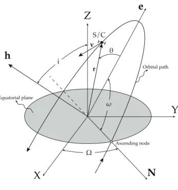
In order to describe the orbit in three dimensions, the orbital plane orientation must be determined with respect to some other reference plane. The geocentric equatorial plane at epoch January 1, 2000 represents the standard in this work. The orthogonal XYZ tern that defines the three-dimensional space is defined by the unit vectors I, J and K. The X axis is aligned as the intersection line between the equator and the ecliptic, commonly known as vernal equinox line, . The Z axis is aligned with the North Pole direction. Finally the Y unit vector comes from the orthogonality between X and Z. Describing the orientation of an orbit in three dimensions requires three additional parameters, called the
Euler angles, which are illustrated in Figure2.4.
First, the intersection of the orbital plane with the equatorial plane is lo-cated. This line is called the node line. The point on the node line where the orbit passes above the equatorial plane from below it is called the ascending node. The node line vector N extends outward from the origin through the as-cending node. At the other end of the node line, where the orbit dives below the equatorial plane, is the descending node. The angle between the positive
e
h
S/C Ω ω θ iX
Z
Y
N
Equatorial plane Ascending node Orbital path r vFigure 2.4: Geocentric equatorial and perifocal frame references with orbital parame-ters and Euler angles
X axis and the node line is the first Euler angle ⌦, the right ascension of the ascending node.
The dihedral angle between the orbital plane and the equatorial plane is the inclination i, measured according to the right-hand rule, that is, counterclock-wise around the node line vector from the equator to the orbit. The inclination is also the angle between the positive Z axis and the normal to the plane of the orbit, h.
It remains to locate the point of closest passage of the orbit. The periapsis lies at the intersection of the eccentricity vector with the orbital path. The third Euler angle !, the argument of perigee, is the angle between the node line vector and the eccentricity vector, measured in the plane of the orbit. In summary, the six orbital elements are:
1. specific relative angular momen-tum, h
2. inclination i
3. right ascension of the ascension node, ⌦
4. eccentricity, e
5. argument of perigee, ! 6. true anomaly, ✓
The transformation from geocentric equatorial to perifocal frame is accom-plished by a sequence of simple Eulerian rotation about the main axis,
illus-trated in Figure2.5. The first rotation, about the Z axis through ⌦, transforms
the X axis into the node line. The second rotation is about the node line through the inclination angle i. The new XY plane is then parallel to the orbital plane. The last rotation, around ˆh and through !, rotates the X’ axis so as it becomes coincident with the periapsis line. The transformation is hence complete and can be formulated analytically by means of the rotation matrices:
R(⌦) = 2 6 6 4 cos ⌦ sin ⌦ 0 -sin ⌦ cos ⌦ 0 0 0 1 3 7 7 5 R(i) = 2 6 6 4 0 0 1 cos i sin i 0 -sin i cos i 0 3 7 7 5 R(!) = 2 6 6 4 cos ! sin ! 0 -sin ! cos ! 0 0 0 1 3 7 7 5 i 2 1 3 3 2 1 2 3 2 i i i 1 1 3 X Y Z Z X Y X’ Y’ X’ Y’ X’ Z Y’ Y’’ Y’’ ˆ h X’ Y’’ ˆ p ˆ p ˆ q ˆ q ˆ h ˆ h
Figure 2.5: Sequence of three rotations transforming I, J, K into ˆe, ˆq, ˆh. The ‘eye’ view-ing down an axis sees the illustrated rotation about that axis. This image is courtesy of Curtis [11]
The result of the rotations sequence is just the product of the transformation matrices for each rotation in the correct order:
RT OT = R(!)R(i)R(⌦) = 2 6 6 4 c⌦c!- s⌦s!ci s⌦c!+ c⌦s!ci sis! -c⌦s!- s⌦c!ci -s⌦s!+ c⌦c!ci sic! s⌦si -c⌦si ci 3 7 7 5
where for notation simplicity c and s stand for cos and sin, respectively. The transformation from perifocal to geocentric equatorial components is
accomplished now thanks to the transpose of this matrix. Let yeq and yperbe
vectors expressed in the geocentric equatorial and perifocal frame, respectively. Then:
yeq = RTT OTyper (2.21)
where the orthogonality property for rotation matrices has been used. 2.3 the restricted three-body problem
This section aims at giving the mathematical formulation and a physical ex-planation on the restricted three-body problem. This model is a better approx-imation of the real dynamics and plays, in this thesis, the role of simplified
reference model. In the case of n = 3 the system of equations (2.2) may be
written as: ¨R1= Gm2 R2-R1 kR2-R1k3 + Gm3 R3-R1 kR3-R1k3 (2.22a) ¨R2= Gm1 R1 -R2 kR1-R2k3 + Gm3 R3 -R2 kR3-R1k3 (2.22b) ¨R3= Gm1 R1-R3 kR1-R3k3 + Gm2 R2-R3 kR2-R3k3 (2.22c)
Equations (2.22) describe the general problem with a set of 18 first order
dif-ferential equations.
The restricted hypothesis requires the mass of the third body to be much
smaller than the masses of the primaries, m3 ⌧ (m2 6 m1). This means the
cluster formed by the primaries actually moves according to Kepler’s laws
and m3 does not influence their motion. The main consequence is that the
barycenter of the system coincides with the m1, m2 pair’s and it moves
obvi-ously in an inertial fashion; it serves therefore for a very convenient reference frame centre. Hereafter the motion of the primaries will be treated as a known
m1 m2 m3 Y Z X R1 R2 R3 r1 r2 ✓
Figure 2.6: Geometry of the three-body problem in an inertial reference frame, XYZ, centred at the primaries barycenter
function of time, R1 =R1(t)and R2 =R2(t). This does not mean that the
prob-lem is incoherent, as is the case of the bicircular four-body probprob-lem. In fact, if the specified functions respect Newton gravitational equations (i. e., ephemeris data), then the problem is still coherent. The third mass particle moves in the
gravitational vectorial field created by the primaries. Note that, if initially m3
has no position and velocity components out of the primaries motion plane, it can but orbit in the same plane.
The dynamics for the third mass particle reads:
¨R = Gm1 R1 -R kR1-Rk3 + Gm2 R2 -R kR2-Rk3 (2.23)
where the subscript 3 referred to the third body has been dropped to simplify the notation.
Another approximation is introduced at this point to simplify the mathemat-ical treatment of the dynamics: the primaries are revolving in circular orbits
on the plane (X, Y) at constant angular speed, !2. The resulting problem is
called circular restricted three-body broblem or CRTBP. Figure 2.6 delineates the
geometry of the problem. Defining a and b the orbital radii of the primary and secondary body, respectively, and the angle between the X reference axis
and the vector from the origin to the smaller primary m2 as ✓ = !2(t - t0),
the circular motion yields R1 = -a(cos ✓, sin ✓, 0)T and R2 = b(cos ✓, sin ✓, 0)T.
The explicit dynamics of R = (X, Y, Z)T 2 R3:
¨X = -G⇣m1 X+ acos ✓ r3 1 + m2 X- bcos ✓ r3 2 ⌘ (2.24a)
¨Y = -G⇣m1 Y+ asin ✓ r31 + m2 Y- bsin ✓ r32 ⌘ (2.24b) ¨Z = -G⇣m1 Z r3 1 + m2 Z r3 2 ⌘ (2.24c) where r1 = q
(X + acos ✓)2+ (Y + asin ✓)2+ Z2 (2.25a)
r2 =
q
(X - bcos ✓)2+ (Y - bsin ✓)2+ Z2 (2.25b)
The dynamics written in the sidereal inertial frame gives birth to a nonau-tonomous set of differential equations whose closed-form solution has not been found yet.
2.3.1 Equations in the synodic frame
The differential system (2.24) describing the motion of a third particle
sub-jected to the gravitational attraction of two primary bodies can be expressed in a more convenient way, which transforms the set of equations in an au-tonomous set. The basic idea is to find a reference frame that results in a time-independent force function. Euler first proposed the synodic frame of reference, this reference is again centered at the primaries’ barycenter but it is rotating so as to maintain the primary bodies at a fixed position in space. For the assumptions made so far the synodic frame rotates at the very same
primaries angular speed, !2. If the axis are the ones shown in Figure 2.7 the
transformation matrix may be straightforwardly written as:
T= 2 6 6 4 cos ✓ - sin ✓ 0 sin ✓ cos ✓ 0 0 0 1 3 7 7 5 (2.26)
Let the third body position vector with respect to the synodic frame be ˆ⇢,
the rotation simply yields R = T ˆ⇢. It’s easy to see that ˆ⇢1 = (-a, 0, 0)T,
ˆ⇢2 = (b, 0, 0)T and ˆ⇢ = (ˆx, ˆy, ˆz)T. By a simple inspection of the geometry
and considering barycentric properties, the positions of the primaries might be expressed as function of the masses and the distance between them.
a= m2
Ml b=
m1
where M is the sum of their masses, M = m1+ m2, and l is their mutual
distance, l = a + b. From Equation (2.23) the dynamics in the synodic reference
becomes: ¨ˆ⇢ + 2TT ˙TT˙ˆ⇢ + TT¨T ˆ⇢ = -G⇣m 1 ˆ⇢ - ˆ⇢1 k ˆ⇢ - ˆ⇢1k3 + m2 ˆ⇢ - ˆ⇢2 k ˆ⇢ - ˆ⇢2k3 ⌘ (2.28) where the properties of a rotation cosine angle matrix have been used, namely the orthonormality and the invariance with respect to the vectorial norm. The derivative of the rotation matrix T are:
˙T = 2 6 6 4 -!2sin ✓ -!2cos ✓ 0 !2cos ✓ -!2sin ✓ 0 0 0 0 3 7 7 5 ¨T = 2 6 6 4 -!2 2cos ✓ !22sin ✓ 0 -!2 2sin ✓ -!22cos ✓ 0 0 0 0 3 7 7 5 (2.29)
Developing the calculations equation (2.28) can be explicitly written per
com-ponents: ¨ˆx - 2!2˙ˆy = !22ˆx - G ⇣ m1ˆx + a ˆ⇢3 1 + m2ˆx - b ˆ⇢3 2 ⌘ (2.30a) ¨ˆy + 2!2˙ˆx = !22ˆy - G ˆy
⇣m1 ˆ⇢3 1 +m2 ˆ⇢3 2 ⌘ (2.30b) ¨ˆz = -Gˆz⇣m1 ˆ⇢3 1 + m2 ˆ⇢3 2 ⌘ (2.30c)
where ˆ⇢1 and ˆ⇢2 are the norm of the distances between the third mass and the
primaries. ˆ⇢1 = q (ˆx + a)2+ˆy2+ˆz2 (2.31a) ˆ⇢2 = q (ˆx - b)2+ ˆy2+ˆz2 (2.31b)
Note that the differential equations now do not depend directly on time and the set is hence autonomous. Furthermore, the physical parameters that
gov-ern equations (2.30) are not mutually independent. It is shown in Szebehely
[44] that, by a proper adimensionalisation, the restricted problem depends on
only one parameter. The adimensionalisation is such that the distance between the primaries, the angular speed and the sum of their masses is set to a unity value. The choice of the dimensionless quantities is:
⇢= ˆ⇢
a+ b ⌧= !2t µ=
m2
m1+ m2
x
y
z
m
1m
2m
3 μ 1-μρ
13ρ
12ρ
3ω
2Figure 2.7: Synodic reference frame for the CRTBP
With this choice the positions of the primaries are simply ⇢1 = (-µ, 0, 0)T and
⇢2 = (1 - µ, 0, 0)T and the adimensional equations become:
¨x - 2 ˙y = ⌦(3b) /x (2.33a) ¨y + 2 ˙x = ⌦(3b) /y (2.33b) ¨z = ⌦(3b) /z (2.33c)
where the three-body potential function can be expressed as:
⌦(3b)= 1 2(x 2+ y2) +1- µ ⇢1 + µ ⇢2 +1 2µ(1 - µ) (2.34)
The constant term has been added to provide a minimum value to the
poten-tial function, independently of the value µ. Terms ⇢1 and ⇢2 are the scalar
distances between the third mass and the primaries.
⇢1 = q (x + µ)2+ y2+ z2 (2.35a) ⇢2 = q (x - 1 + µ)2+ y2+ z2 (2.35b)
The dimensionless equations (2.33) depend clearly only on the mass parameter,
µ.
The CRTBP written in this form possesses a first integral of motion, called Jacobi integral and named after its discoverer, Jacobi (1836). It can be easily
obtained by manipulating the equations of motion. After multiplying each component by the corresponding velocity and summing:
¨x ˙x - 2 ˙y ˙x + ¨y ˙y + 2 ˙x ˙y + ¨z ˙z = @⌦(3b)
@x ˙x +
@⌦(3b)
@y ˙y +
@⌦(3b)
@z ˙z (2.36)
Since the potential function in the synodic frame does not depend directly on
time, the right-hand side of Equation (2.36) is the total time derivative of ⌦.
The left-hand side might be written as the time derivative of the square speed. Performing an integration:
C= J(x, y, x, ˙x, ˙y, ˙z) = 2⌦(3b)(x, y, z) - ( ˙x2+ ˙y2+ ˙z2) (2.37)
According to the formalism in [33] and [46], the Jacobi integral represents a
five-dimensional manifold for the particle state in the six-dimensional phase space. It reduces therefore the possible motion to the hypersurface:
J-1(C) = {(x, y, x, ˙x, ˙y, ˙z) 2 R6| J- C = 0} (2.38)
where C = J(x0) is the Jacobi constant associated with the initial condition
x0 = (x0, y0, x0, ˙x0, ˙y0, ˙z0)T. Moreover, thanks to the semi-definite positiveness
of the kinetic term, it must be 2⌦ > J, where the equality is valid only when
the kinetic energy is zero. The Jacobi integral can be hence used to establish some allowed and forbidden regions for the motion of the third particle once initial conditions are specified. These regions are bounded by the Hill’s surfaces, on which the velocity of the mass particle is identical null. The zero-velocity surfaces are defined in the configuration space by
⌦-1(C) = {(x, y, x) 2 R3 | 2⌦(3b)(x, y, z) - C = 0} (2.39)
The Jacobi integral is directly related to the total energy E of the third body
J= -2E (2.40)
which states that a high value for the Jacobi constant means a low energy at disposal. It’s intuitive to think that, as the Jacobi constant decreases, the third body starts possessing enough energy to escape the gravitational attraction of the primaries.
2.3.2 Lagrangian points
Any set of numbers (x, y, z, ˙x, ˙y, ˙z)T satisfying the Jacobi equation C =
2⌦(3b)(x, y, z) - ( ˙x2+ ˙y2+ ˙z2) represents a possible motion for a given value
of the constant C4. The six-dimensional manifold
G(x, y, z, ˙x, ˙y, ˙z) = C - 2⌦(x, y, z) + ( ˙x2+ ˙y2+ ˙z2) = 0 (2.41)
possesses singularities at points where partial derivatives of the manifold are zero.
G/x = 0 G/y= 0 G/z= 0 (2.42a)
G/˙x = ˙x = 0 G/˙y= ˙y = 0 G/˙z= ˙z = 0 (2.42b)
The last three conditions entail the singularities reside on the surface of zero ve-locity, where C = 2⌦(x, y, z). The manifold singularities are then those points where
⌦/x = 0 ⌦/y = 0 ⌦/z= 0 C= 2⌦ (2.43)
It is important to note that the singularities of the manifold do not correspond to the singularities of the equations of motion, located instead at both pri-maries and infinitely away from the origin. What is more, the singularities of the manifold of the states of motion, when input in the dynamics, give rise to a null acceleration field, ¨x = ¨y = ¨z = 0. It can be demonstrated by simple inspection, that in these points all the successive time derivatives of the com-ponents are zero. If the third particle is placed at an equilibrium point with zero velocity, it will stay there. For this reason the singularities of the manifold are equilibrium points for the third body dynamics and are often called station-ary points, libration points or Lagrangian points. These special points are widely known in literature and have been studied thoroughly for their interesting
dy-namical and phase space portrait (see Section 1.3). A tool to determine the
position of the Lagrangian points, addressed as Li, will be presented. The
con-ditions expressed by Equations (2.43) in expanded form are:
⌦/x = x -(1 - µ)(x + µ) ⇢31 -µ(x - 1 + µ) ⇢32 = f(x, y, z) = 0 (2.44a) ⌦/y = y(1 -1- µ ⇢3 1 - µ ⇢3 2 ) = y· g(x, y, z) = 0 (2.44b) ⌦/z= -z(1- µ ⇢3 1 + µ ⇢3 2 ) = z· h(x, y, z) = 0 (2.44c)