Analysis of the aerosol number size distribution variability and characterization of new particle formation events at Monte Cimone GAW global station

(1)

Scuola di Scienze

Corso di Laurea Magistrale in Fisica del Sistema Terra

Analysis of the aerosol number size

distribution variability and

characterization of new particle formation

events at Monte Cimone GAW global

station

Relatore:

Prof. Federico Porcù

Correlatori:

Dott. Angelo Lupi

Dott.ssa Angela Marinoni

Candidata:

Martina Mazzini

Sessione III

(2)

(3)

To better assess how aerosols impact on Earth system, the observations of ultrafine particle number concentration and their size distribution in different location and environments are crucial, especially in remote sites, like high altitude mountain sites, where the atmosphere is representative of baseline conditions.

The aim of this thesis is to obtain long-term information on aerosol number size distribution and new particle formation (NPF) at the Mt. Cimone GAW global station (CMN, 2165 m a.s.l.). The size distribution of particles ranging from 9nm to 500nm was continuously observed with a DMPS from November 2005 to July 2013 in the framework of EUSAAR and ACTRIS European projects. Size distribution and number concentration are studied at different time scales, together with occurrences of NPFs. CMN typical aerosol number size distribution is bimodal. On average, CMN aerosol population features a total number concentration of 1534_{± 1332cm}−3. The number concentration shows large seasonal variations with higher values during warm months, almost four times higher than those observed in winter. On a daily time scale, the maximum of total particles occurs in the afternoon. When classifying aerosol number size distribution into nucleation mode (9-25nm), Aitken mode (25-100nm), and accumulation mode (100-500nm), Aitken mode is the main contributor to the total number concentration for about 53%, followed by particles in the accumulation and nucleation modes with 31% and 16%, respectively.

According to the procedure laid down by Kulmala et al., 2012 NPFs are identified by distinguishing each day following standardised classification criteria. CMN is characterized by a NPF events frequency of 26.7%, with the highest event occurrence in May and August, while non-events are more frequent during winter. The growth of nucleation mode particle and the time evolution of the nucleation number concentration begin, on average, around local noon. The first one lasts almost three hours, with a mean growth rate of 4.65± 1.97 nm/h, while the latter lasts more than one hour and a half, with a rate of 0.50_{± 0.56 cm}−3s−1. The average condensation sink is 0.280·10−3_s−1 _{during a typical non-event day, and 0.483·10}−3_s−1 _{during a}

typical event day. However, low CS observed before the nucleation onset time can be an important factor triggering NPFs, except during winter season.

(4)

(5)

Una migliore comprensione degli effetti degli aerosol sul sistema climatico beneficia di osservazioni a lungo termine della concentrazione del numero di particelle ultrafini e della loro distribuzione dimensionale in luoghi ed ambienti diversi. Questo vale, in particolare per siti remoti, come quelli ad alta quota, dove l’atmosfera è rappresentativa delle condizioni di background a larga scala.

Lo scopo di questa tesi è ottenere informazioni sulla variabilità delle osservazioni di distribuzione dimensionale in numero degli aerosol e sugli eventi di formazione di nuove particelle (NPF) osservati presso la GAW Global Station di Monte Cimone (CMN, 2165 m s.l.m.). La distribuzione dimensionale di particelle con dimensioni comprese tra 9 nm e 500 nm è stata continuamente monitorata tramite un DMPS, a partire da Novembre 2005 fino a Luglio 2013, nell’ambito dei progetti europei EUSAAR e ACTRIS. In questo elaborato, la distribuzione dimensionale e la concentrazione numerica vengono analizzate considerando scale temporali differenti, insieme agli eventi di NPF.

La distribuzione numerica dimensionale tipica del sito CMN risulta bimodale. In media, la popolazione di aerosol ha una concentrazione totale di 1534± 1332cm−3. L’andamento tipico annuale della concentrazione numerica presenta un massimo estivo, quasi quattro volte superiore ai valori osservati mediamente in inverno. Su scala giornaliera, il numero massimo di particelle si osserva nel pomeriggio, molto più accentuato in estate rispetto alle altre stagioni. Suddividendo lo spettro della distribuzione numerica dimensionale nella moda di nucleazione (9-25 nm), nella moda di Aitken (25-100 nm) e nella moda di accumulazione (100-500 nm), la moda di Aitken è quella che contribuisce maggiormente alla concentrazione totale con circa il 53%, seguita dalle mode di accumulazione e nucleazione che contribuiscono rispettivamente con il 31% e il 16%.

Secondo la procedura stabilita da Kulmala et al., 2012, abbiamo identificato gli eventi di NPF, classificando ogni giorno in base a criteri di classificazione noti in letteratura. Presso il sito CMN si registra una frequenza di eventi di NPF del 26.7%, con la più alta presenza di eventi nei mesi di Maggio e Agosto, mentre i non-eventi sono più frequenti durante l’inverno. Nei casi di NPF più chiari, abbiamo studiato la crescita delle particelle nella moda di nucleazione e l’aumento di concentrazione, che iniziano ogni giorno mediamente intorno al mezzogiorno locale. In media, la crescita in diametro dura quasi tre ore, con una velocità di 4.65±1.97nm/h, mentre la crescita in concentrazione dura più di un’ora e mezza, con un rate di 0.50± 0.56cm−3_s−1_. Il condensation sink medio è 0.280· 10−3_s−1 _{durante una tipica giornata non-evento,} mentre ha un valore medio di 0.483_·10−3_s−1 _{durante una giornata in cui avviene NPF.} Viene osservato un CS basso prima che la nucleazione abbia inizio, ad eccezione della stagione invernale. Ciò significa che CS può essere considerato un fattore importante per innescare il meccanismo di NPF.

(6)

(7)

Introduction

Aerosol particles can influence the Earth radiation budget by scattering and absorbing sunlight (direct effect). They can also affect Earth albedo by serving as cloud condensation nuclei (CCN) and ice nuclei (IN), and thus they can influence cloud formation and lifetime as well (IPCC, 2013). The cloud albedo effect of aerosols is one of the biggest uncertainties in global climate models (IPCC, 2013), and strongly depends on the number concentration and size distribution of particles. Numerous studies have focused on monitoring the particle number size distribution (PNSD) within the planet boundary layer (PBL), where anthropogenic sources have strong impacts (Peng et al., 2014). However, particles in the pristine free troposphere (FT) have rarely been studied. Mountain sites are located far from anthropogenic emissions and thus they are the ideal sites for monitoring the temporal variations of aerosols in the atmosphere at background levels.

The overall aim of this thesis is to enrich the information of aerosol concentration and size distribution by analyzing the longest Italian record gathered by the mountain ground based station O. Vittori at Mt. Cimone (2165 m a.s.l.). This station is the only one among the 31 Global Stations of the Global Atmospheric Watch (GAW) program set up by the World Meteorological Organization (WMO) present on the Italian territory and in the Mediterranean Basin. The aerosol number size distribution observation at Mt. Cimone was implemented in the frame of EUSAAR FP6 program, in November 2005, and it has been continuously carried out also in the frame of ACTRIS-FP7 and ACTRIS-2-H2020 programs. This site represents a strategic platform to study the climatology of the free troposphere in the South Europe and the Mediterranean basin. For these reasons, its contribution to extent the view of particle number concentration and size distribution within observational networks is fundamental.

To accomplish this aim, size distributions data collected from a differential mobility particle sizer (DMPS) from November 2005 to July 2013 are analyzed. In particular, information about diurnal, seasonal, annual and inter-annual variability of aerosol number concentration and size distributions is obtained. Then, a study of new particle formation (NPF) is carried out. New particle formation is estimated to provide the 45% of global cloud condensation nuclei, but the abundance of nucleated particles responds

(12)

other environmental factors that are still not completely understood (Merikanto et al., 2009). In order to understand the phenomenon of NPF at Mt. Cimone, we first need to know its frequency and characteristics. For this reason, in the present work a preliminary detailed investigation of NPF event and non event is carried out.

Chapter one provides the most relevant information on tropospheric aerosol. It

contains a description of the main sources and removal mechanisms and offers an overview of aerosol particles physical, chemical and electrical properties. This Chapter depicts the key aspects of current knowledge about their impact on visibility, health, and climate. Finally, it deepens into the new particle formation mechanisms and main evolutionary processes to which aerosol particles are subjects in the atmosphere.

Chapter two contains a detailed description of the measurement site and the

methodology of NPSD observation and data analysis. First of all, the chapter provides a presentation of the O. Vittori atmospheric observatory managed by the National Research Council of Italy. Then, a description of the operating principles of the DMPS, used to measure the aerosol size distribution, is given. Finally, the methods adopted to process raw data and to create a homogeneous data set together with the complete analysis procedure used to analyze it are explained.

Chapter three reports the main results obtained by studying the available data.

Starting from a description of the data set obtained through the preprocessing of raw data, the third chapter proceeds with the long-term characterization of the aerosol population measured at Mt. Cimone. The properties of the aerosol population are investigated by outlining the diurnal, monthly, seasonal, and interannual differences in size distributions and number concentrations. Then, the total aerosol number concentration recorded at Mt. Cimone is compared with that observed at other stations in a global context. Finally, the results concerning the observation of new particle formation are reported. In particular, the characteristics of events occurring at Mt. Cimone are studied and compared to those observed at other high altitude ground based sites, which performed experimental NPF studies providing an overall picture of the frequency of occurrence of the process and of some events features.

(13)

Atmospheric aerosol

Atmospheric aerosol is a suspension of fine solid particles or liquid droplets in air, ubiquitously present in the Earth’s atmosphere. The term aerosol commonly refers to aerosol particles.

Emitted directly as particles (primary aerosol) or formed in the atmosphere by gas-to-particle conversion processes (secondary aerosol), atmospheric aerosol particles range in size from a few nanometers (nm) to tens of micrometers (µm) in diameter. They play an important role influencing the energy balance of the Earth’s system, visibility, climate, human health and environment as a whole. In spite of the great efforts made by the scientific community in the last decades, the atmospheric aerosol still presents unknowns due to its large variability and complexity in terms of sources, transport and transformation mechanisms, chemical composition, size distribution, global distribution and interaction with other components of the Earth’s system.

This chapter summarizes the present knowledge on aerosols properties, impacts and new particle formation mechanisms in the atmosphere.

1.1 Aerosol life cycle

1.1.1 Sources and formation

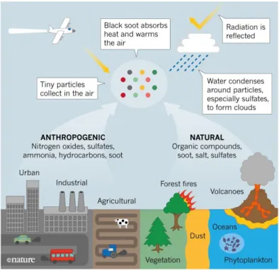
A way to classify aerosol particles is based on their origin. Aerosol can originate from natural sources and anthropogenic sources (Boucher, 2015). Particles emitted from both natural and anthropogenic sources are given in Table 1.1.

Significant natural sources of particles include volcanic activity, wind-driven soil erosion processes, sea spry, biomass burning, and reactions between natural gaseous emissions.

Emissions of particulate matter attributable to the activities of humans arise primarily from four source categories: fuel combustion, industrial processes, nonindustrial fugitive sources (roadway dust from paved and unpaved roads, wind erosion of cropland, construction, etc.) and transportation sources (automobiles, etc.)

(14)

(Seinfeld and Pandis, 2016).

Figure 1.1: Diagram of the role and sources of atmospheric aerosols in

the atmosphere, showing emmission processes and the action of aerosol while in the atmosphere (Penner, 2019).

Aerosols can also be classified according to their formation processes into two groups: primary aerosols and secondary aerosols.

Primary aerosols are particles emitted or injected directly into the atmosphere, and they can have both natural origins, like salt from the sea, dust from dry regions, or particles released by wildfires, and anthropogenic origins, like particulate resulting from fuel combustion, transport activities and industrial processes.

Secondary aerosols are particles formed via gas to particle conversion, in which condensable vapours lead either to growth of preexisting particles by condensation processes, or nucleation of new particles (Tomasi, Fuzzi, and Kokhanovsky, 2017). The phenomenon involving the nucleation of gas-phase atmospheric components into newly-formed particles, as well as their subsequent growth and coagulation, is called atmospheric new particle formation (NPF) (Kalkavouras et al., 2021). Such process is important since it represents the first step in the complex processes leading to formation of cloud condensation nuclei and it has a major influence on the radiative balance of the global climate system. NPF will be treated in details in Section 1.4 since it is a fundamental topic for the work that has been carried out in this thesis.

(15)

Source Particle size (µm)

Emission (Tg/yr)

Natural

Primary Soil dust (mineral aerosols); D<1 110

D=1-2 290

D=2-20 1750

Sea to air flux of sea salt; D<1 54

D=1-16 3290

Biogenic organic matter; Coarse 1000

Volcanic ash; Fine 20

Secondary Sulfate from aerosols from Fine 16-32

marine biogenic gases (mainly DMS);

Sulfate from aerosols form Fine 57

terrestrial biogenic gases;

Nitrate aerosols from N Ox Mainly 3.9

(lightining, soil microbes); coarse

Organic matter from biogenic gases; Fine 16

Sulfate aerosols from volcanic SO2; Fine 9-21

Natural

subtotals At least 6600

Anthropogenic

Primary Aerosols from all kinds of fossil Coarse 100

fuel burning, cement manufacturing, and fine metallurgy, waste incineration, etc;

Soot (black carbon) from fossil Fine 8

fuel burning (coal, oil);

Soot from biomass burning; Fine 5

Biomass burning without soot; Fine 80

Secondary Sulfate from SO2 (mainly from coal Fine 140

and oil burning);

Nitrate aerosol from N Ox (fossil Mainly 36

fuel and biomass combustion); coarse

Organic matter from anthropogenic Fine 5

gases;

Organic matter from biomass Fine 54

burning;

Organic matter from fossil fuel Fine 28

burning;

Anthropogenic

subtotals 460

Total 7100

Table 1.1: Natural and anthropogenic sources of primary and secondary

aerosols in global scale [based on Maenhaut, 1996; Raes et al., 2000; Mather et al., 2003; Jaenicke, 2005]. Adapted from (Wang, 2010).

(16)

1.1.2 Removal

The atmospheric life of aerosol particles emitted by the primary sources or formed from the precursor gases is schematically illustrated in Figure 1.2 and it is regulated by nucleation, coagulation, and condensation processes which will be explained in detail in Section 1.4. Subsequently, aerosol removal may occur through dry and wet deposition.

Figure 1.2: Schematic representation of the sequence of processes

involving the atmospheric life of aerosol particles after the emission of the precursor gases, until their removal from the atmosphere through dry

deposition and wet (rainout) mechanisms (Tomasi, Fuzzi, and Kokhanovsky, 2017).

The most important removal process for submicron aerosols is wet deposition, also called wet scavening (Xu et al., 2019), defined as the removal of any material from the atmosphere to the Earth’s surface by the precipitation of liquid or frozen hydrometeorites. Arimoto et al. [1985] have measured a contribution of the aerosol wet deposition flux to the total deposition flux in the Pacific of 70 to 90% for trace elements, far from their source region. In a rural area, i.e., closer to source areas, Prakasa Rao et al. [1992] measured wet deposition flux contributions of 74 and 62% for sulfate and nitrate aerosols, respectively. In regions far from the sources, where the largest particles have already been removed by gravitational settling, this contribution has been estimated to be 60 to 85% for desert dust (Guelle et al., 1998). Two processes lead to wet deposition: the nucleation scavenging and the impaction scavenging. The former mechanism refers to aerosols (cloud condensation nuclei: CCN) inducing formation of cloud droplets in supersaturated water vapour and the latter mechanism refers to collision-coalescence of aerosols and water droplets. The impaction scavenging usually splits in two processes: in-cloud impaction scavenging, which treats the

(17)

interactions between cloud droplets and raindrops with interstitial aerosol particles (particles too small to nucleate to cloud droplets) and below cloud scavenging, which concerns the collection of aerosol particles by falling raindrops below the cloud base. The relative importance between in-cloud scavenging processes (nucleation and impaction scavenging), also called washout, and below cloud scavenging, also called rainout, depends on meteorological conditions and on the properties of aerosol particles (size distribution and chemical composition) as well as on the stage of cloud development (Berthet et al., 2010). Scavenged aerosols are irreversibly removed from the atmosphere if the water droplets gravitationally fall and reach the ground.

If wet deposition is an eﬀicient sink for aerosols, it is of course conditional on the presence of precipitating clouds whose spatial and temporal distribution is very heterogeneous. Some regions experience very little precipitation while other regions exhibit very strong seasonal variations in precipitation (Boucher, 2015). In the absence of precipitation, the direct deposition of aerosols and aerosol precursors onto the Earth’s surface, called dry deposition, becomes important. The relative importance of the removal effects by dry deposition depends on various factors, such as the atmospheric turbulence level, the chemical and water solubility characteristics of the particles, and surface and terrain characteristics. In fact, the level of turbulence governs the rate at which aerosols are delivered down to the surface, especially within the layer nearest to the ground, such a rate varying as a function of aerosol size, density, and morphological characteristics. The surface roughness constitute also a very important factor in dry deposition, since a smooth surface may lead to particle bounce-off, and canopies generally promote dry deposition (Tomasi, Fuzzi, and Kokhanovsky, 2017). Many investigators have chosen to represent the overall dry deposition process in terms of three simplified steps (Hosker Jr and Lindberg, 1982; Hicks et al., 1987). The first step is the aerodynamic transport by turbulent diffusion down through the atmospheric surface layer until to a very thin layer of stagnant air just adjacent to the surface. The second step is the Brownian transport across this thin stagnant layer of air until reaching the surface, called the quasi-laminar sublayer. Finally, the last step is the uptake of particles, which adhere to the surface, whose moisture and stickiness are important factors. Each of the steps can occur at a different rate; the slowest step generally determines the overall rate of dry deposition (Wu et al., 1992).

(18)

1.2 Physical and Chemical Aerosol Properties

1.2.1 Morphology and size characterization

Particulate matter is commonly characterized by its size. The latter can be defined as geometric or physical diameter (dp) at the simplest level. If the particle is spherical

the meaning of this parameter is obvious, otherwise it does not have a precise meaning and atmospheric aerosol particles are often nonspherical (DeCarlo et al., 2004). In fact, atmospheric particles can be characterised by various shapes: from the rough-edge shape of a crustal particle in Figure 1.3a, to the long branched chains of small nanoparticles characterizing Diesel exhausts emission in Figure 1.3b, to the flat appearance of a skin fragment in Figure 1.3c, to the cubic shape of a sodium chloride crystal in Figure 1.3d (Perrino, 2010).

Figure 1.3: Shapes of atmospheric particles. Photos by courtesy of

Prof. Y. Mamane, Technion, Haifa (Israel) (Perrino, 2010).

Nonspherical particles are generally characterized by equivalent diameters, defined as the diameter of a sphere, which with a given instrument would yield the same size measurement as the particle under consideration (DeCarlo et al., 2004). For exemple, the equivalent volume diameter (de) is defined as the diameter of a sphere

of the same volume as that of the irregular particle. Also commonly used is the aerodynamic diameter (da). This is defined as the diameter of a spherical particle with

unit density which has the same settling velocity as the particle in question (Baron and Willeke, 2001). Aerodynamic diameter is useful for characterising particles with significant inertia, which are typically particles larger than 0.5µm. Smaller particles undergo Brownian motion and diffusion diameter is used for them. Diffusion diameter is defined as the diameter of a spherical particle with density of unity which has the

(19)

same diffusion as the particle in question (Salimi, 2014). However, for the aim of the thesis it is fundamental to introduce the electrical mobility diameter (Dp), since all the data analyzed in the present work were obtained by a Differential Mobility Particle Sizer (DMPS) which classifies charged particles according to their mobility in an electric field. The instrument will be described in detail in Chapter 2. Electrical mobility diameter is defined as the diameter of a spherical particle with unit density which has the same electrical mobility (Zp) as the particle in question (Flagan, 2001).

The behavior of a particle in an electric field is deepened in Section 1.3.3, where the equation of the electric mobility is derived. The equation of the electrical mobility diameter is the following:

Dp = neCc

3πηZp

(1.1) where n is the number of excess elementary charges e carried by the particle, η is the viscosity of air and Cc is the Cunningham slip corrector factor (Kulmala et al., 2012).

For spherical particles, Dp equals dp and de (DeCarlo et al., 2004).

1.2.2 Ultrafine, Fine and Coarse Modes

Taking into account the size characterization explained in the previous paragraph, this chapter assumes spherical aerosols of a known diameter Dp and density ρp, in order

to provide a single coherent mathematical description of the particles. Aerosol sizes span several orders of magnitude, from a few nanometers for new particles produced by nucleation, to several hundred micrometers for the largest particles produced by the wind friction on the land and the ocean surface (Boucher, 2015). Particles less than 2.5µm in diameter are generally referred to as fine and those greater than 2.5µm diameter as coarse (Seinfeld and Pandis, 2016).

Fine and coarse particles differ in sources, formation mechanisms, composition, atmospheric lifetimes, spatial distribution, indoor–outdoor ratios, and temporal variability. Therefore the distinction between fine and coarse particulate matter is a fundamental one in any discussion of the physics, chemistry, measurement, or health effects of aerosols.

Fine particles can be divided roughly into three modes: the nucleation mode with a particle diameter Dp < 25nm (also called the ultrafine mode), the Aitken mode 25nm < Dp < 100nm (named after the Scottish meteorologist and physicist John Aitken), the accumulation mode 100nm < Dp < 2, 5µm. The nucleation particles mainly form through condensation of hot vapors during combustion processes and/or nucleation of atmospheric gaseous species to form fresh particles and they are lost principally by coagulation with larger particles.

The accumulation mode is so named because mass accumulates in this size range by coagulation of particles in the nuclei mode and condensation of vapors onto existing

(20)

particles.

The coarse mode is formed by mechanical processes and usually consists of man-made and natural dust particles. A supercoarse mode can be found close to the source point but is generally absent in more aged aerosol populations.

1.2.3 Size Distribution

The size of aerosol particles affects both their lifetime in the atmosphere and their physical and chemical properties (Seinfeld and Pandis, 2016). It is therefore necessary to develop methods of mathematically characterizing aerosol size distributions. A measured distribution of particle sizes can be described by a histogram of the number of particles per unit volume within defined size bins. By making the bin sizes tend to zero a continuous function is formed called the diameter number density distribution N (Dp) which represents the number of particles with diameters between Dp and Dp + ∆Dp per unit volume. The differential diameter number density distribution nN(Dp) is

defined by

nN(Dp) =

dN (Dp)

dDp . (1.2)

The same equation can be written in integral form as

dN (Dp) =

∫ Dp+∆Dp Dp

nN(Dp)dDp. (1.3)

The total number of particles per unit volume N is given by

N =

∫ _∞ 0

nN(Dp)dDp. (1.4)

Several aerosol properties depend on the particle surface area and volume distributions with respect to particle size. So it is important to define the aerosol surface area distribution as

nS(Dp) = πDp2nN(Dp) (1.5)

and the aerosol volume distribution

nV(Dp) =

π

6Dp 3_n

N(Dp). (1.6)

The observed aerosol distribution is fitted reasonably well by log-normal distribution, the most useful in situations where the distributed quantity can have only positive values and covers a wide range of values. Therefore, atmospheric aerosol size

(21)

distributions can be described as the sum of n log-normal distributions nN(logDp) = n ∑ i=1 N0,i √ 2πlogσg,i exp ( −1 2

(logDp− logDpg,i)2

log2_σ

g,i

)

(1.7)

where N0,i is the integral of the ith lognormal function, Dpg,i is the mean geometric

diameter, and σg,i is the geometric standard deviation of the ith log-normal mode.

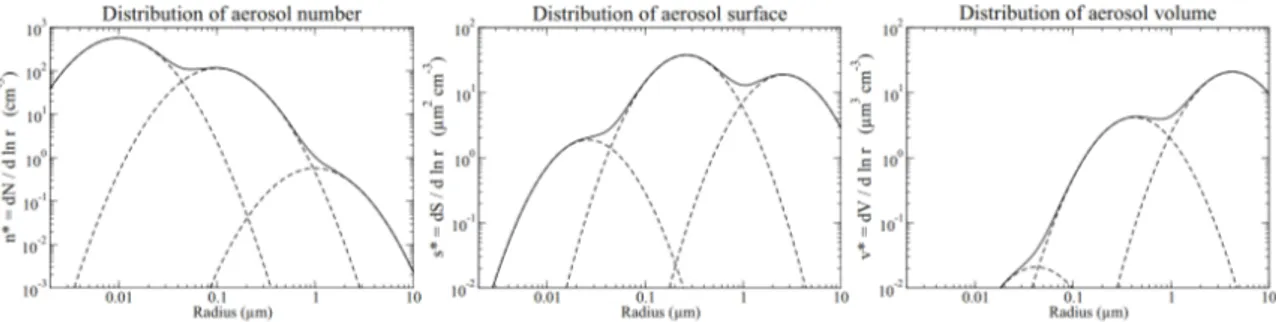
Figure 1.4: Schematic of the three modes of the aerosol size distribution

(Boucher, 2015).

Figure 2.9 shows the superposition of three log-normal distributions with mean geometric number radius rg of 0.01, 0.1 and 1µm, geometric standard deviation

σg of 2 and with total concentrations of 1000, 200 and 1cm−1, respectively. This

illustration shows how the fine mode dominates the aerosol number distribution, while the accumulation mode dominates the aerosol surface distribution and the coarse mode dominates the aerosol volume. The ultrafine and supercoarse modes that may also exist are not represented in this schematic.

1.2.4 Chemical composition

The chemical composition affects aerosol properties like radiative effects, hygroscopic growth, reactivity, ability to form cloud droplets, and, consequently, their effects on the environment, from visibility impairment to effects on human health and from effects on the biosphere to material deterioration and to climate change (Tomasi, Fuzzi, and Kokhanovsky, 2017).

Primary aerosol

Primary aerosols are atmospheric particles that are emitted directly into the atmosphere and consist of both inorganic and organic components. Inorganic primary aerosols are relatively large (often larger than 1µm) and originate from sea spray, mineral dust, and volcanoes. Primary organic aerosols (POA) sources include biomass/fossil fuel combustion, higher plants and soil dust. Some examples of POA are primary biological aerosol particles (PBAPs) such as pollen, spores, bacteria, plant and

(22)

animal fragments. These coarse aerosols have short atmospheric lifetimes, typically only a few days.

Secondary aerosol

Secondary aerosols are mainly composed by sulfate, nitrate, ammonium ions and secondary organic carbon, especially in the finest fractions. The secondary aerosols concentration depends on concentrations of precursor gasses or other reactive gaseous species, such as O3 and radical OH, and on atmospheric conditions.

Sulfate aerosols are a suspension of fine solid particles of a sulfate (SO2−

4 ) or tiny droplets of a solution of a sulfate or of sulfuric acid (hydrogen sulfate). They are produced by chemical reactions in the atmosphere from gaseous precursors, with the exception of sea salt sulfate and gypsum dust particles. The two main sulfuric acid precursors are sulfur dioxide (SO2) from anthropogenic sources and volcanoes, and dimethyl sulfide (DM S) from biogenic sources, especially marine phytoplankton. Ammonium (N H+

4 ) is the principle cation associated with fine sulfate and fine nitrate in the continental aerosol. Ammonia (N H3) is released by natual soils, coal combustion, biomass burning, fertilizer application and production or is emitted as a result of the decay of waste products from domestic animals, wild animals, seas and oceans (Wang, 2010).

Nitrate (N O₃−) is often found in both fine and coarse atmospheric aerosol particles. Nitrate in fine particles is produced from the reaction of gas-phase nitrate (nitric acid;

HN O3) and ammonia (N H3) (Kim, 2019). Nitrate in coarse particles comes primarily from the reaction of gas-phase nitric acid with pre-existing coarse particles. Typical sources of nitric oxides are fossil fuel combustion, soils, biomass burning and lightning. Secondary organic aerosols (SOA) components are formed by chemical reaction and gas-to-particle conversion of volatile organic compounds (V OCs). Formation of

V OCs from the gas phase can be both natural and anthropogenic. The main natural compounds are isoprene, monoterpenes and sesquiterpenes while the main anthropogenic are aromatics, alkanes and alkenes. The SOA formation can then be due to nucleation and growth of aerosol particles, adsorption and absorption of V OCs by preexisting aerosols or cloud particles, heterogeneous and multi-phase chemical reaction of V OCs or semi-volatile organic compounds (SV OC), at the surface or in the bulk of aerosol or cloud particles. There are still many uncertainties in emission and processes involving P OA and SOA, which reflects in a lack of knowledge about their concentration and role in the climate system (Renzi, 2019).

(23)

Geographic Distibution

Long-term aerosol mass concentrations are measured systematically at the surface by global and regional networks. A survey of the main aerosol types can be constructed from such measurements. Figure 1.5, taken from the IPCC report Climate Change 2013, shows bar chart plots summarizing the mass concentration (µgm–3_{) of seven} major aerosol components for particles with diameter smaller than 10µm, from various rural and urban sites in six continental areas of the world with at least an entire year of data and two marine sites. Mineral dust dominates the aerosol mass over some continental regions with relatively higher concentrations especially in urban South Asia and China. In the urban North America and South America, organic carbon (OC) contributes the largest mass fraction to the atmospheric aerosol, while in other areas of the world the OC fraction ranks second or third. Sulfate is an important component of the inorganic fraction of the aerosol, and is systematically accompanied by ammonium. Nitrate can be present in very variable quantities but concentrations decrease rapidly outside source regions. Sea salt can be dominant at oceanic remote sites with 50 to 70% of aerosol mass (IPCC 2013).

Figure 1.5: Climatology of the mass concentrations (µgm−3_{) of seven}

major chemical species of the atmospheric aerosol in different regions of the world. Reproduced from Boucher, 2015. (© IPCC)

(24)

1.3 Electrical Properties

In aerosol mechanics, the most important electrostatic effect is the force exerted on a charged particle in an electrostatic field (Hinds, 1999). Most aerosol particles carry some electric charge since they are formed, but they can also be charged during their life cycle or, artificially, using specific tools, like particle charger, where ions are mixed with the aerosol sample. This is a fundamental property because the motion induced by electrostatic forces forms the basis for important type of air-cleaning equipment and aerosol sampling and measuring instruments. Indeed, all the data analyzed for the present thesis where collected using a Differential Mobility Particle Sizer (DMPS), described in detail in Chapter 2. The DMPS operating principle is based on the charging of collected particulate through a particle charger and the application of an electric field in order to classify charged particles according to their electrical mobility. In this section some charging mechanism observable in nature by which particle acquire charge are described. Among them, the diffusion charging mechanism is exploited by the Neutralizer, described in 2.2.2, which is part of the Differential Mobility Particle Sizer used at Mt. Cimone. Then, the definition of the so called Boltzmann

equilibrium of charge distribution is given and the concept of the electric mobility,

already introduced in Section 1.2.1, is examined more closely.

1.3.1 Charging mechanism

The principal mechanisms by which aerosol particles acquire charge are flame charging, static electrification, field charging, and diffusion charging. The last two require the production of unipolar ions and are used to produce highly charged aerosols. Most of the information of this paragraph is taken from (Hinds, 1999).

Flame charging occurs when particles are formed in or pass through a flame. At

the high temperature of the flame, direct ionization of gas molecules creates high concentrations of positive and negative ions and thermionic emissions of electrons or ions from particles. Indeed, flames generate large numbers of ions and charged clusters with concentrations as high as 1010_/cm3 _{(Wang et al., 2017). The highly} concentrated ions and charged clusters actively collide with the formed nanoparticles, adding electrostatic potentials to the system, and further altering the properties of the generated particles, such as their size, shape, and crystallinity (Zhang et al., 2012).

Static electrification causes particles to become charged by mechanical action as

they are separated from the bulk material or other surfaces. Particles are usually charged by static electrification during their formation, resuspension, or high-velocity transport. The three primary mechanisms of static electrification that can charge aerosol particles during their generation are electrolytic charging, when a liquids

(25)

with a high-dielectric constant are separated from solid surfaces, spray electrification, when the surface of some liquids is disrupted during the formation of droplets by atomization or bubbling, and contact charging, when a particle contacts a surface, charge is transferred between the particle and the surface.

Field charging is charging by unipolar ions in the presence of a strong electric field.

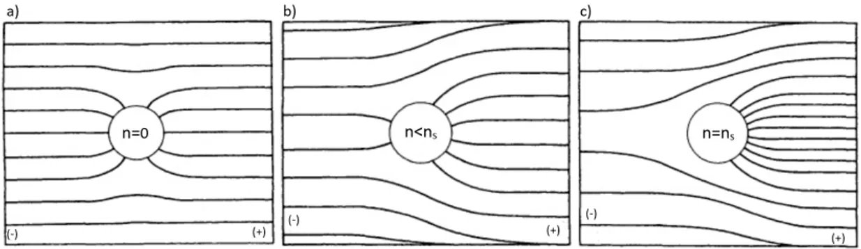
This mechanism is depicted in Figure 1.6, in which the negatively charged plate is at the left and negative ions are present. When an uncharged spherical particle is placed in a uniform electric field, it distorts the field, as shown in Figure 1.6a. The field lines shown represent the trajectories of ions. For an uncharged particle, the greater the value of ϵ, the greater the number of field lines that converge on the particle. Ions in this electric field travel along the field lines and collide with the particle where the field lines intersect the particle and transfer their charge to it. As the particle becomes charged, it will tend to repel the like-charged incoming ions, as shown in Figure 1.6b. The rate of ions reaching the particle decreases as the particle becomes charged. Ultimately, the charge builds up to the point where no incoming field lines converge on the particle, as in Figure 1.6c, and no ions can reach the particle. At this maximum-charge condition, the particle is said to be at saturation charge.

Figure 1.6: Electric field lines for a conductiong particle in a uniform

field with a negative plate at left. a) An uncharged particle. b) A partially charged particle. c) A particle at saturation charge. (Hinds,

1999).

According to Hinds, 1999, the number of charges, nf ield, acquired by a spherical particle

of diameter Dp during a time t in an electric field Ecwith an ion number concentration

Ni is nf ield(t) = ( 3ϵ ϵ + 2 )( Ecπϵ0D2p e )( πeZiNit 4πϵ0+ πeZiNit ) (1.8) where Zi is the electric mobility of ions and ϵ0 is the permittivity of the vacuum. In this equation the first two factors represent the saturation charge ns reached after

suﬀicient time at a given charging condition:

ns = ( 3ϵ ϵ + 2 )( Ecπϵ0D2p e ) (1.9)

(26)

The rate of charging does not depend on the particle size or field strength, but only on the ion concentration. When particles are intentionally charged by field charging, the ion concentration is usually 107_/cm3 _{or greater, so charging will be 95% complete} in 3 s or less.

Finally, particles mixed with ions become charged by random collisions between the ions and the particles. This process is called diffusion charging because the collisions result from the Brownian motion of the ions and particles. This mechanism does not require an external electrical field and, to a first approximation, does not depend on the particle material. As the charge accumulates, it produces a field that tends to repel additional ions, reducing the charging rate. The ions, being in equilibrium with the gas molecules, have a Boltzmann distribution of velocities. As the charge on the particle increases, fewer and fewer ions have suﬀicient velocity to overcome the repulsive force, and the charging rate slowly approaches zero. It never reaches zero, however, because the Boltzmann distribution of velocities has no upper limit. An approximate expression taken from Hinds, 1999, for the number of charges ndif f(t)

acquired by a spherical particle of diameter Dp by diffusion charging during a time t

is ndif f(t) = 2πϵ0DpkT e2 ln ( 1 + Dpcie 2_N it 8ϵ0kT ) (1.10) where ϵ0 is the permittivity of the vacuum, k is the Boltzmann constant, T is the temperature, e is the charge of the elementary charge, ci is the mean thermal velocity

of the ions and Ni is their concentration. Although theoretical charging equations, such

as the above, are usually valid for spherical particles only, the particle diameter is often substituted by mobility equivalent diameter. Even in the presence of an electrostatic field, diffusion charging is the predominant mechanism for charging particles less than 0.2µm in diameter (Hinds, 1999).

1.3.2 Equilibrium charge distribution

Uncharged particles are rare because of random collisions with the omnipresent air ions. Indeed, every cubic centimeter of air contains about 103 _{ions with approximately equal} numbers of positive and negative ions (Epa, 2004). Aerosol particles that are initially neutral will acquire charge by collision with ions due to their random thermal motion. Aerosol particles that are initially charged will lose their charge slowly as the charged particles attract oppositely charged ions. These competing processes eventually lead to an equilibrium charge state called the Boltzmann equilibrium charge distribution. The latter represents the charge distribution of an aerosol in charge equilibrium with bipolar ions. For equal concentrations of positive and negative ions, a reasonable first approximation for normal air, the fraction of particles fn of a given size having n

(27)

positive (or n negative) elementary units of charge is given by fn = exp(KEn2e2/DpkT ) ∑_∞ n=−∞exp(KEn2e2/DpkT ) (1.11) where KE = _4πϵ1₀ is the Coulomb’s constant equal to 9.0· 109N · m2/C2. For particle

diameters Dp larger than 0.01µm, over 99% of the particles carry no charges when they

are at the Boltzmann equilibrium charge distribution. The percentage of uncharghed particles drops to 42.6% for 0.1µm particles, 13.5% for 1µm particles, and 4.3% for 10µm particles (Wang, 2005).

1.3.3 Motion of a particle in an external field

To derive the equation of motion for a particle of mass mp, let us begin with a force

balance on the particle, which we write in vector form as

mp dv dt = ∑ i Fi (1.12)

As long as the particle is not moving in a vacuum, the drag force will always be present, so let us isolate the drag force from the summation of forces

mp dv dt = 3πµDp Cc (u− v) +∑ i Fei (1.13)

where Fei denotes external force i (those force arising from external potential fields,

such as gravity and electrical forces) and Cc is the Cunningham slip corrector factor.

If a particle has an electric charge q in an electric field of strength E, an electrostatic force Fee = qE acts on the particle. The equation of motion for a particle of charge q moving at velocity v in a fluid with velocity u in the presence of an electric field of

strength E is mp dv dt = 3πµDp Cc (u− v) + qE (1.14) At steady state in the absence of a background fluid velocity, the particle velocity is such that the electrical force is balanced by

ve = qCc

3πµDp

E (1.15)

where veis termed the electrical migration velocity. Finally, we can define the electrical mobility of a charged particle Zp as

Zp =

neCc

3πηDp

(28)

The electrical mobility of a particle is defined as the ratio of the constant limiting velocity a charged particle will reach in a uniform electric field to the magnitude of this field (Kulkarni, Baron, and Willeke, 2011).

1.4 Impacts

1.4.1 Climate effects

One of the driving reasons for the analysis provided in this thesis is the important role aerosol particles play in the climate system. The new terminologies adopted in this paragraph can be found in the Fifth Assessment Report (AR5) of the Intergovernmental Panel on Climate Change. Indeed, the IPCC report of 2013 pointed out the importance of distinguishing between the traditional concept of radiative forcing (RF) and the relatively new concept of effective radiative forcing (ERF) that also includes rapid adjustments. In the next paragraph the concept of rapid adjustment is analysed more in detail. RF, in units of W m−2_{, is defined, as it was in the Fourth} Assessment Report AR4 of 2007, as the instantaneous perturbation in net radiative flux at the tropopause exerted by a change in a component of the radiative budget, with surface temperature and tropospheric state maintained in their unperturbed state. By convention, negative RFs denote a decrease in net radiative flux, or a loss of energy from the climate system. Conversely, positive RFs denote a gain of energy to the climate system. ERF represents the change in net downward radiative flux at the top of the atmosphere after allowing for atmospheric temperatures, water vapour and clouds to adjust, but with global mean surface temperature or a portion of surface conditions unchanged. So, ERF is the sum of RF and its fast adjustments, and it is a better predictor of the subsequent long-term change in surface temperature than instantaneous RF (Bellouin, 2014).

Forcing, Rapid Adjustments and Feedbacks

Aerosols can be defined as forcing agents, which are elements of the climate system with the ability to influence the global mean surface temperature by acting on the Earth’s energy balance. This action can be direct or driven by rapid adjustaments. The latter, sometimes called rapid responses, arise when forcing agents, by altering flows of energy internal to the system, affect cloud cover or other components of the climate system and thereby alter the global budget indirectly. Adjustments can occur through geographic temperature variations, lapse rate changes, cloud changes and vegetation effects. These adjustments are generally very quick and do not operate through changes in surface temperature, that are slowed by the ocean’s heat capacity. The effect on climate of forcing agents can then be amplified or decreased through feedback mechanisms

(29)

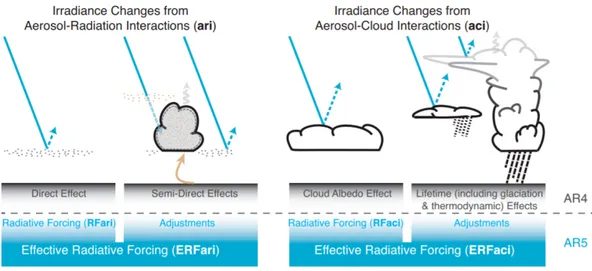
or changes in climatic variables mediated by a variation in the global mean surface temperature which impact on radiative budget. For aerosols, the IPCC report of 2013 distinguishes forcing processes arising from aerosol–radiation interactions (ari), and aerosol–cloud interactions (aci), whose global impact are respectively defined as Effective Radiative Forcing from aerosol-radiation interaction (ERFari) and Effective Radiative Forcing from aerosolcloud interaction (ERFaci). Both these components of the change are divided into Radiative Forcing and adjustments as in Figure 1.7. The blue arrows depict solar radiation, the grey arrows terrestrial radiation and the brown arrow symbolizes the importance of couplings between the surface and the cloud layer for rapid adjustments.

Figure 1.7: Schematic of the new terminology used in the Fifth

Assessment Report (AR5) for aerosol–radiation and aerosol–cloud interactions and how they relate to the terminology used in Fourth

Assessment Report AR4.

Aerosol–Radiation Interactions

The radiative effect due to aerosol–radiation interactions (RFari), formerly known as direct radiative effect, is the change in radiative flux caused by the combined scattering and absorption of radiation by anthropogenic and natural aerosols. A schematic representation of the aerosol radiation interaction is shown in Figure 1.8. Aerosols increase the reflection of solar radiation back to the space through various radiative and physical processes. Moreover, a small fraction of them is also capable of heating the lower atmosphere when they contain energy absorbers likely elemental carbon and mineral dust. RFari depends on the horizontal and vertical distributions of aerosol concentrations and scattering and absorption properties, which in turn depend on aerosol sizes and chemical composition. Environmental factors, such as the solar zenith angle, and the reflectance of the surface or cloud underlying the aerosol layer, also play important roles. Approximate formulas to quantify RFari at the Top of the

(30)

Atmosphere in cloud-free sky have been derived, such as the following (Bellouin, 2014), which is valid for both scattering and absorbing aerosols:

RF ari∼ ST2ω0β∆τ [(1− Rs)2− 2Rs(1− ω0/(βω0)] (1.17) where S is the solar constant, in W m−2, T is the dimensionless transmittance of the atmosphere above the aerosol layer, and Rs is the dimensionless reflectance of the

surface. Aerosols are characterized by three dimensionless parameters: the change in optical thickness, ∆τ ; the single scattering albedo ω0; the upscatter fraction, β, which quantifies the fraction of radiation that is scattered upward with respect to the particle’s horizontal plan. Equation 1.17 highlights the fact that the sign of RFari depends on the aerosol absorption properties and the reflectance of the surface. It also shows that for a given set of optical properties, RFari depends linearly on the change in aerosol optical thickness or, equivalently, aerosol concentrations.

Figure 1.8: Schematic representation of scattering and absorption by a

single particle.

Aerosol–radiation interactions give rise to rapid adjustments, which are particularly pronounced for absorbing aerosols such as BC. Indeed, aerosols that are highly absorbing of solar radiation may reduce cloud cover and liquid water content by heating the cloud and the environment within which the cloud forms. This is known as the semi-direct effect (Hansen, Sato, and Ruedy, 1997) because it is the result of direct interaction of aerosols with radiation but also influences climate indirectly by altering clouds.

Aerosol–Cloud Interactions

The radiative forcing due to aerosol–cloud interactions (RFaci), termed alternatively aerosol first indirect RF, cloud albedo forcing, or Twomey forcing in the scientific

(31)

literature, arises from the role aerosols play in the hydrological cycle as cloud condensation nuclei. Cloud droplets are formed by the condensation of water on already existing aerosol particles called cloud condensation nuclei (CCN ). The presence of suitable particles in the air greatly reduces the supersaturation needed to form water droplets and hence clouds. The ability of a particle to act as a nucleus for water droplet formation (i.e., to become activated as a CCN ) depends on size, chemical composition, and the local supersaturation. Hygroscopic materials such as sulfates and sea salts are especially eﬀicient as CCN ; mineral dust and combustion products can also be effective, especially if they are wet or have hygroscopic coatings. Organic substances have also been recognised as active cloud condensation and ice formation nuclei. Increased numbers of CCN s, recognised by several studies summarized in the IPCC report (2007), lead to more cloud droplets and a concurrent decrease in droplet sizes and it is called Twomey effect. The non-linear relationship derived in Feingold and Graham, 2003, between the concentrations in number of aerosols and raindrops is as follows:

Nd∼ (Na)b (1.18)

where Nd is the drop concentration, Na is the total particle concentration and b can

vary widely, with values ranging from 0.06 to 0.48 (low values of b correspond to low hygroscopicity), because of the great sensitivity to the characteristics of the aerosol. An approximate formula for the computation of RFaci proposed by Bellouin et al. (2014) is: RF aci∼ −S · f · δα δNd · δNd δNa · dNa (1.19)

where S is the solar constant, f is the fractional cloud cover, δNa is the change in

cloud condensation nuclei due to anthropogenic activities, δNd/δNa is the sensitivity

of cloud droplet number, Nd, to a change in cloud condensation nuclei, and δα/δNd is

the susceptibility of cloud albedo, α, to a change in cloud droplet number.

Efforts to understand the other component of the ERFaci, cloud adjustments, have been similarly clouded in uncertainty (Douglas and L’Ecuyer, 2020) and are associated with both albedo and so-called lifetime effects. Because of multiple light scattering within the cloud, the cloud albedo tends to increase with increased numbers of CCN. In addition, models have shown that aerosol affects the distribution of liquid throughout the cloud and vertical motion within the cloud, greatly perturbing the cloud’s lifetime, precipitation, and extent (Ramanathan et al., 2001). Aerosol can act to increase the lifetime of clouds through delayed collision coalescence, or decrease the lifetime through evaporation-entrainment (Small et al., 2009). The cloud adjustment response depends on the cloud state and a sequence of reactions dictated by the environment (Gryspeerdt et al., 2019). Indeed, observational evidence for fast adjustments is mixed, with observations showing either a reduction or enhancement of precipitation in regions

(32)

with high anthropogenic aerosol loading, depending on cloud regime. For example, aerosol-driven fast adjustments are unlikely to influence those clouds whose lifetime is not regulated by precipitation, such as nonprecipitating stratocumulus clouds. At the other end of the precipitation spectrum, clouds where accretion of raindrops dominates over autoconversion (the initial stage of the collision–coalescence process whereby cloud droplets collide and coalesce to form drizzle drops) are also not likely to be influenced by aerosol-driven changes in cloud droplet size distribution. Aerosol fast adjustments would then be limited to specific cloud regimes, or to situations where increases in cloud condensation nuclei forces a change in cloud regime, such as the transition from open to closed-cells cumulus clouds (Bellouin, 2014).

Summary of Effective Radiative Forcing

The quantification of interactions in the cloud-aerosol-radiation system remains elusive and the recent IPCC report stresses that aerosol climate impacts remain the largest uncertainty in driving climate change. The table reported in Figure 1.9 has an overview of the RF agents considered in the previous paragraphs and each of them is given a confidence level for the change in RF over the Industrial Era to 2011. The confidence level is based on the evidence (robust, medium, and limited) and the agreement (high, medium, and low) as given in the table. The basis for the confidence level and change since AR4 is provided. Note that the confidence level for aerosol–cloud interactions includes rapid adjustments. For aerosol–radiation interaction the table provides separate confidence levels for RF due to aerosol–radiation interaction and rapid adjustment associated with aerosol–radiation interaction.

Figure 1.9: Confidence level for the forcing estimate associated with

each forcing agent for the 1750–2011 period (Adapted from IPCC 2013.

In the IPCC report of 2013, the ERF due to aerosol–radiation interactions that takes rapid adjustments into account (ERFari) is assessed to be –0.45_{±0.5W m}–2_{. The}

(33)

uncertainty estimate is wider but more robust, based on multiple lines of evidence from models, remotely sensed data, and ground-based measurements. The total ERF due to aerosols (ERFari+aci, excluding the effect of absorbing aerosol on snow and ice) is assessed to be be –0.9W m–2 _{with a 5 to 95% uncertainty range of –1.9 to} –0.1W m–2 _{(medium confidence), and a likely range of –1.5 to –0.4W m}–2_{. This range} was obtained from expert judgement guided by climate models that include aerosol effects on mixed-phase and convective clouds in addition to liquid clouds, satellite studies and models that allow cloud-scale responses.

(34)

1.4.2 Health effects

Numerous epidemiological studies show that fine air particulate matter and traﬀic-related air pollution are correlated with severe health effects, including enhanced mortality, cardiovascular, respiratory, and allergic diseases (Bernstein et al., 2004). Moreover, toxicological investigations in vivo and in vitro have demonstrated substantial pulmonary toxicity of model and real environmental aerosol particles, but the biochemical mechanisms and molecular processes that cause the toxicological effects such as oxidative stress and inflammatory response have not yet been resolved. Epidemiological studies usually refer to PM mass concentrations, but some health effects may relate to specific constituents such as bioaerosols, polycyclic aromatic compounds, and transition metals (Shiraiwa et al., 2017). Global modeling combined with epidemiological exposure-response functions indicates that ambient air pollution causes about 4.3 million of premature deaths per year, of which 4.04 million due to

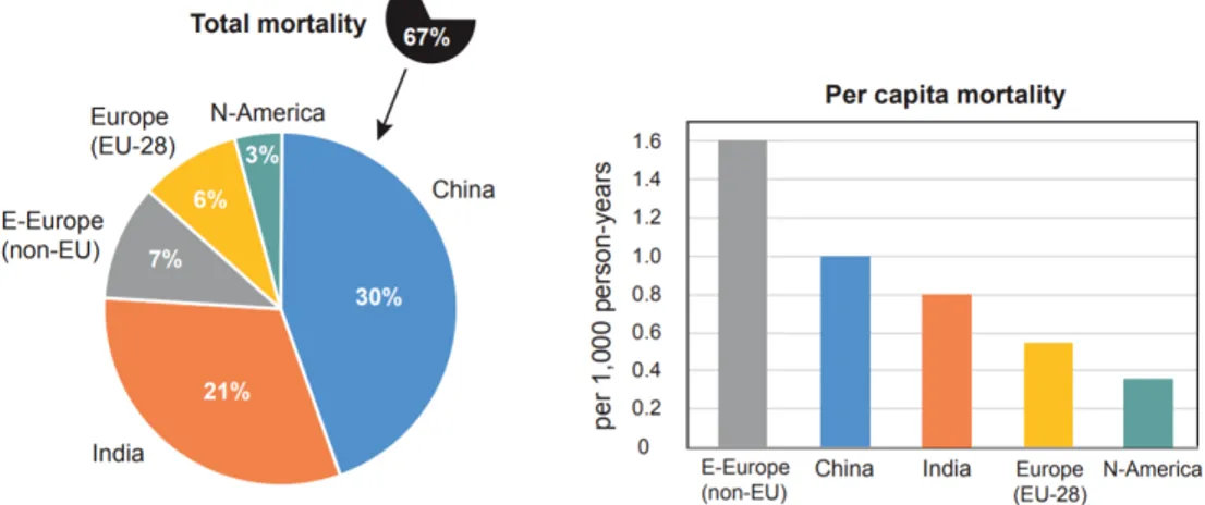
P M2.5 (particulate matter with diameter lower than 2.5µm). The uncertainty on this estimate is 25% (95% confidence interval) (Chowdhury et al., 2020). The mortality, however, is not equally distributed throughout the globe; people who live in low and middle income countries disproportionately experience the burden of pollution with 91% of premature deaths occurring there, in particular in South-East Asia and Western Pacific regions. The 70% occurs in Asia, and more than 50% in China and India alone. Although the majority of deaths occur in these countries, per capita mortality is higher in Eastern Europe, as can be seen in the Figure 1.10.

Figure 1.10: About two-thirds of the global mortality attributable to

air pollution of 4.3 million/year occur in China, India, Europe and N-America (left). Though China and India lead in terms of total mortality, the per capita mortality is highest in Eastern Europe (right)

(35)

1.4.3 Visibility effects

Visibility degradation is the most observable impact of air pollution and considered as a primary and general index of ambient air quality in an urban area (Watson, 2002). The term visibility may be defined as the farthest distance an object can be seen against the sky from the horizon (Seinfeld and Pandis, 2016). This depends on several factors such as optical properties of the atmosphere, amount and distribution of light, characteristics of the objects and properties of the human eye (Seinfeld and Pandis, 2016). Both particles and gases interact with light, and the interactions consist of light absorption and light scattering. These two processes, scattering (changes the direction of photon) and absorption (removes the photon from the beam by conversion to thermal or electronic energy) are collectively known as light extinction and responsible for visibility reduction. According to the mechanisms leading to the attenuation of light, the light extinction coeﬀicient, bext, is usually conceived as comprising:

bext = bsp+ bsw+ bsg+ bap+ +bag (1.20)

where bsp is the component due to scattering of light by particles, bsw is the component

of scattering of light due to moisture in the air; bsg is the Rayleigh scattering by clean

air, bap is the component due to absorption of light by particles and bag is mainly due

to the absorption of light by N O2 gas (Chan et al., 1999).

Gaseous scattering has minor contribution to visibility reduction in urban areas whereas scattering and absorption by atmospheric particles have been found to be more prominent reason of light extinction in urban areas (Chan et al., 1999). The effect of particulates on visibility is further complicated by the fact that particulates of different sizes are able to scatter light with varying degrees of efficiency (Malm, 1999). It is of interest to investigate the efficiency with which an individual particle can scatter light. The efficiency factor is expressed as a ratio of a particle’s effective cross section (sum of scattering and absorption cross sections ssca _{and s}abs_{) to its}

geometrical cross section sg:

Qext =

ssca_{+ s}abs

sg

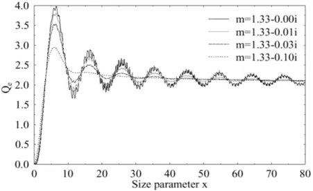
(1.21) Figure 1.11 shows how this eﬀiciency varies as a function of particle size parameter (or Mie parameter) defined as

x = 2πr

λ (1.22)

where r is the radius of the particle and λ is the wavelength under consideration. Very small particles and molecules are very ineﬀicient at scattering light. As a particle increases in size, it becomes a more eﬀicient light scatterer until, at a size that is close to the wavelength of the incident light, it can scatter more light than a particle five

(36)

times its size.

Figure 1.11: Examples of Qextcalculated with the Mie theory for several refractive indexes.

A further reduction of visibility depends on ambient relative humidity (RH), which has a great impact on aerosol optical properties (Deng et al., 2016). Atmospheric aerosols can be categorized into hygroscopic aerosols and non-hygroscopic aerosols. Hygroscopic aerosols include sulfates, nitrates, ammonium, sea salt and other inorganic components, as well as some water soluble organic compounds (WSOC), whereas, the chemical composition of non-hygroscopic aerosols mainly includes black carbon and some organic compounds. For ambient atmosphere, hygroscopic aerosols take up water as humidity increases (Engelhart et al., 2011). Aerosol water can affect both the size and refractive indices of atmospheric aerosols, thereby influencing the mass concentration, size distribution, and corresponding optical properties (Malm and Day, 2001). Relative humidity in the ambient atmosphere sees significant diurnal and seasonal changes. When RH reaches 70–80%, water content of aerosols can generally contribute 50% or more of the fine particle mass, becoming a controlling factor in aerosol optical properties as light scattering becomes greater with enlarged particular size (Bohren and Huffman, 2008). Hence visibility may be low on days with high aerosol loading and when humidity is high. Since rain scavenges aerosol particles from the atmosphere, some of the best visibility days occur after strong rain events.

(37)

1.5 New Particle Formation

Atmospheric new particle formation (NPF) and growth involves the formation of molecular clusters and their subsequent growth to larger sizes, first to a few nm in particle diameter, then to nucleation and Aitken mode particles in the sub-100 nm size range, and possibly up to sizes at which these particles may act as cloud condensation nuclei (CCN) (Kerminen et al., 2018). While the aerosol formation has been observed to take place almost everywhere in the atmosphere (Kulmala et al., 2012), serious gaps in our knowledge regarding to this phenomenon still exist. These gaps include existence and dynamics of atmospheric molecular clusters, vapours participating on atmospheric cluster formation, the effect of those clusters on atmospheric nucleation, the effect of ions on particle formation and also various impacts of the new particle formation on atmospheric chemistry, climate, human health and environment (Sipilä et al., 2008).

Figure 1.12: Schematic presentation of the main processes affecting

atmospheric particle formation and growth (Olenius et al., 2018).

Formation and evolution in time of natural and anthropogenic aerosols are influenced by gas-to-liquid phase transitions. The formation process of a liquid phase from the vapor can usually be divided into three steps. First, a small amount of the new phase is formed spontaneously (nucleation). Secondly, an increasing amount of the new phase accumulates around the initially formed nuclei (condensational growth). Further particle growth is finally caused by collision and coalescence of the droplets

(38)

(coagulation). Depending on the actual physical situation, two or even all three of these processes can occur simultaneously. In the following paragraphs the processes of formation and growth, shown in Figure 1.12, are described.

1.5.1 Atmospheric Vapor and Particle Formation

As already mentioned in Chapter 1, secondary aerosols are particles formed via gas to particle conversion in which condensable vapours lead either to growth of preexisting particles by condensation processes or nucleation of new particles (Tomasi, Fuzzi, and Kokhanovsky, 2017). Atmospheric gas-to-particle conversion requires vapors whose ambient concentrations exceed their equilibrium vapor concentration, also referred to as volatility, over the condensed-phase particles. In practice, gas-phase chemical production of condensing vapors or rapid changes in the environmental parameters, such as the temperature, is necessary to initiate NPF. The vapors known to contribute to NPF include sulfuric acid (H2SO4) and a variety of oxidized organic species, together with basic compounds and water (Olenius et al., 2018).

Nucleation theory

Nucleation is the transformation of matter from one phase to another phase through the formation of nuclei. It is the initial stage of a first-order phase transition that takes place in various energetically metastable or unstable systems (Colbeck and Lazaridis, 2014). For atmospheric aerosols, nucleation refers to the transformation of gas-phase molecules into a cluster of molecules called an aerosol embryo or an aerosol nucleus (Boucher, 2015). Nucleation is responsible for production of the tiniest particles due to gas-to-particle conversion (Bychkov, Golubkov, and Nikitin, 2010). This process is sometimes called homogeneous nucleation to distinguish it from the process of heterogeneous nucleation where the phase change occurs on a pre-existing surface (Boucher, 2015). Classical nucleation theory to describe aerosol formation still forms the basis for the thermodynamic interpretation of aerosol nucleation processes. The fundamental concepts of the theory are described according to Curtius, 2009. The Gibbs free energy G is studied to characterize the atmospheric nucleation processes as the natural variables pressure and temperature can easily be measured. For a given, fixed pressure and temperature, a closed thermodynamic system will drive towards a state in which G is minimal. Let us start by looking at the nucleation process in the simplest case of a single substance A, for example, pure sulphuric acid. Substance A has a vapour pressure pA. Its equilibrium vapour pressure over a flat surface of the bulk

liquid A is pA∞. If the substance is supersaturated in the gas phase (pA > pA∞) and

far away from any other surfaces on which the gas phase molecules could condense on, the system is meta-stable and the vapour molecules would generally prefer to undergo