1. GREEN’S FUNCTIONS IN LAYERED MEDIA 1.1. Introduction

(1)

1. GREEN’S FUNCTIONS IN LAYERED MEDIA

1.1. Introduction

In a variety of applications as remote sensing, geophysical prospecting, microstrip circuits and antennas, it is necessary to evaluate the electromagnetic field in layered media. For a given set of sources, the field can easily be found if the Dyadic Green’s Functions (DGFs) of the environments are available.

When the currents are not known a priori, which is usually the case of scattering and antenna problems, the DGFs can be used to formulate integral equations for the true or equivalent currents, which are then solved numerically by the Method of Moments (MoM) [1].

The hypersingular behavior of some of the integral equation kernels causes difficulty in the solution procedure [2] which can be avoided if the field is expressed in terms of the vector and scalar potentials with weakly singular kernels. This leads to the development of Mixed-Potential Integral Equations (MPIEs) for arbitrary shaped scatterers in free space [3]. In layered media, an important advantage of the MPIEs is that the spectral Sommerfeld-type integrals appearing in the potential kernels converge more rapidly and are easier to accelerate than those associated with the field forms that are, in effect, obtained by differentiation of the potentials. On this basis, the MPIEs formulation proposed by K. A. Michalski and R. Mosig in [4] has been employed. In the above mentioned approach, a compact representation of the electric and magnetic-type DGFs is provided for plane stratified, multilayered uniaxial medium.

In order to evaluate each dyad component, an equivalent transmission-line along the axis normal to the stratification is used and the MPIEs kernels are developed in this framework. The DGFs in the wave-number domain are expressed in terms of currents and voltages defined on the equivalent network. The space domain counterparts are then expressed in closed form by applying the Sommerfeld Identity.

Attention is limited to media with at most uniaxial anisotropy which, while being important in practice, still allow the use of the simple transmission-line models for the electromagnetic fields.

In the following sections, the adopted procedure will be described in details, giving particular emphasis to the MPIEs formulation as well as to the numerical and theoretical aspects regarding the approximation of the

(2)

spectral functions by using the Generalized Pencil of Function (GPOF) method [5].

1.2. Spectral Domain Green’s Functions

Let us consider a general shaped object embedded in a layered medium where the fields (E,H) are generated by known electric and magnetic currents (Ji, Mi) (Fig. 1.1).

Figure 1.1. General shaped object embedded in a layered medium.

An external equivalent problem is shown in Figure 1.2 where the same sources, together with the surface currents (JS, MS), produce the original fields (E, H) outside the object surface S and null inside.

Figure 1.2. External equivalent problem for the object embedded in a layered medium.

Since:

(3)

where (Ei, Hi) are the impressed fields due to (Ji, Mi) and (ES, HS) are the scattered fields due to (JS, MS). Applying the boundary condition at S yields:

(

)

(

)

ˆ , , ˆ , s i s s s S s i s s s S M n E E J M J n H H J M + +   = − ×_ + _   = ×_ + _ (1.2)

where ˆn is the outward unit vector normal to S and the superscript S+ indicates that the fields are evaluated as the observation point approaches S from the exterior region.

In a linear medium the fields generated by (J, M) can be expresses as:

, , , , , EJ EM HJ HM E G J G M H G J G M = + = + (1.3)

where GPQ

(

r r| '

)

is the DGFs relating P-type field in r and Q-type current

in r’, while the symbol 〈⋅ ⋅〉, represents an integral inner product.

Since it is possible to calculate the DGFs of the equivalent medium reported in Fig. 1.2, (1.3) can be used to express the scattered fields (1.2) in terms of the unknown currents (JS, MS). However, since in layered media the scalar potential kernels associated with vertical and horizontal current components are in general different, the formulation proposed by Michalski and Mosig introduces a scalar potential correction factor to consider general current distributions:

(

)

(

)

' 0 0 ' 0 0 1 ˆ , , , , , 1 ˆ , , , , A EM HJ F E j G J K J C z J G M j H G J j G M K M C z M j φ φ ψ ψ ωµ ωε ωε ωµ = − + ∇ ∇ ⋅ + + = − + ∇ ∇ ⋅ + (1.4)

where µ0, ε0 are the free-space permeability and permittivity, the prime

over the operator nabla indicates that the derivatives are performed with respect to the source coordinates, A

G , GF, Kφ,Kψ, Cφ and Cψ are the

magnetic and electric vector potentials, the corresponding scalar potential kernels and the correction factors associated with the electric and magnetic longitudinal current distributions respectively [4].

(4)

Let us consider a transverse unbounded medium with respect to z axis characterized by a z-depended complex permeability:

ˆˆ , ˆˆ t t t z t z I zz I zz µ µ µ ε ε ε = + = + (1.5) where t

I represents the unit transverse dyadic.

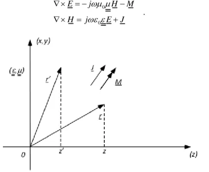
The fields (E,H) generated by the source currents (J,M) at an arbitrary point r are expressed by the Maxwell’s equations (Fig. 1.3):

0 0 . E j H M H j E J ωµ µ ωε ε ∇× = − − ∇× = + (1.6)

Figure 1.3. Current radiating in an uniaxial medium.

Since the medium is of infinite extent in the transverse direction

ˆ ˆ

xx yy

ρ = + , the analysis can be facilitated expressing all the field component f(ρ;z) through their Fourier transform with respect to the transverse coordinate:

(

k_ρ;z

)

F f

( )

;z f

( )

;z ejkρρdxdy , ψ ρ ∞ ∞ ρ ⋅ −∞ −∞   = _ _=

∫ ∫

(1.7 (a))

(5)

( )

1

(

)

_{( )}

(

)

2 1 ; ; ; , 2 jk x y f ρ z F ψ k_ρ z ψ k_ρ z e ρρdk dk π ∞ ∞ − ⋅ − −∞ −∞   = _ _=

∫ ∫

(1.7 (b)) where kρ =k x_xˆ+k y_yˆ.

Applying the (1.7(a)-(b)) to (1.6), the analysis can further be simplified defining a rotate reference system

(

k z k_ρ;ˆ× _ρ

)

in the wave-number domain with unit vector u vˆ ˆ, defined by (Fig. 1.4):

ˆ ˆ ˆ . ˆ ˆ ˆ y x y x k k u x y k k k k v x y k k ρ ρ ρ ρ = + = − + (1.8)

Figure 1.4. Rotated wave-number domain coordinate system.

Appling (1.8) to (1.6) and separating the longitudinal and transverse parts of the resulting equations, one obtains:

(

)

(

)

0 0 ˆ . ˆ z z t z z z t z j E jk H z J j H jk z E M ρ ρ ωε ε ωµ µ − = ⋅ × + − = ⋅ × +       (1.9)

(6)

where: 0 0 0 0 , . , t t t t e h z z t k k k ε µ ν ν ε µ µ ε ω µ ε = = = = (1.10)

If one expresses the transverse electric and magnetic fields as:

ˆ ˆ , ˆ ˆ ˆ e h t e h t E uV vV H z uI vI = + × = +   (1.11)

and projects them on the new reference system, two transmission-line equations of the following form are obtained:

, p p p p p z p p p p p z dV jk Z I v dz dI jk Y V i dz = − + = − + (1.12)

where p can represents e or h. Therefore, the transverse electric and magnetic fields in the new coordinate system can be interpreted as voltages and currents on an equivalent transmission-line along the z axis (Fig. 1.5). The line propagation constant, characteristic impedance and admittance read like:

2 2 0 0 1 , 1 p p z t e e z e t h t h h z k k k k Z Y Z Y k ρ ν ωε ε ωµ µ = − = = = = (1.13)

where the square root branches in (1.13) is simplified by the condition:

( )

arg k_zp 0 .

π

− < ≤ (1.14) The current and voltage sources in (1.12) are given by:

(7)

0 0 , . , e e z u z h h z u z k J M i J k i M J v M ρ ν ρ ν ν ωε ε ωµ µ = − = − = − − =       (1.15)

Figure 1.5. Equivalent transmission-line.

In view of (1.9)-(1.11), the electric and magnetic fields in the spectral domain can be express as:

0 0 ˆ ˆ ˆ , ˆ ˆ ˆ e z e h z h z h e z jk I J E uV vV z j jk V M H uI vI z j ρ ρ ωε ε ωµ µ + = + − − = − + +     (1.16)

which indicates that the original vector problem (Fig. 1.3) is thus reduced to two scalar transmission-line ones associated with the Transverse Magnetic (TM) and Transverse Electric (TE) partial fields.

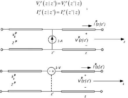
In order to find the solutions of the transmission-line equations (1.12), let Vip(z|z’) and Iip(z|z’) denote the voltage and current at z due a to 1-A

source current at z’ while let Vvp(z|z’) and Ivp(z|z’) denote the voltage and

current at z associated with a 1-V source voltage at z’ (Fig. 1.6). Then, the Transmission-Line Green’s Functions (TLGF’s) satisfy the following relations:

(

)

(

'

)

, ' p p p p p p p p i i z i z i p p p p p p p p v v z v z v dV dI jk Z I jk Y V z z dz dz dV dI jk Z I z z jk Y V dz dz δ δ = − = − + − = − + − = − (1.17)

(8)

where δ is the Dirac distribution. The previous quantities meet the following reciprocity properties:

(

)

(

)

(

)

(

)

| ' ' | , | ' ' | p p i i p p v v V z z V z z I z z I z z = = (1.18)

Figure 1.6. Network problems for the evaluation of the transmission-line Green’s functions.

(

)

(

)

(

)

(

)

| ' ' | . ' | | ' p p v i p p i v V z z I z z I z z V z z = − = − (1.19)

The linearity of equations (1.12) allow to evaluate the voltages and the currents at any z by using the superposition integrals:

, , . , , p p p p p i v p p p p p i v V V i V v I I i I v = + = + (1.20)

Substituting the (1.20) into (1.15) and (1.16), the spectral domain dyadic Green’s functions can be express as:

' 0 0 ˆ ˆ ˆ ˆ ˆ ˆ ˆ ˆ , h e i v HJ h e i i z z zvk V vzk I G uvI vuI ρ ρ ωµ µ ωε ε = − − + +  _{(1.21 (a))}

(9)

(

)

' 0 0 2 ' 0 0 ˆ ˆ ˆ ˆ ˆ ˆ ˆ ˆ . ˆˆ ' e e i v EJ e h i i z z e v z z zuk I uzk V G uuV vvV k I zz z z j j ρ ρ ρ ωε ε ωε ε δ ωε ε ωε ε = − − + + + +  − −       (1.21 (b))

The above formulation does not make any assumption on the z-dependency of the layer parameters. The presented procedure will be now specialized to the case of a multilayered medium with constant parameters for each layer. The transmission-line analog, for this particular situation, consists of a cascade of uniform transmission-line sections, where the nth element is characterized by a propagation constant kznp, a characteristic

impedance Znp and terminals zn and zn+1 (Fig. 1.7).

Figure 1.7. Voltage and current point sources in the nth_{transmission-line section.}

In order to compute the resulting voltage and current at z in section m, the transmission-line has been excited with unit-strength voltage and current in section n at z’. The parameters p

n

Γ and p n

Γ , denoting the voltage reflection coefficient looking to the left and right of the nth section respectively, can be evaluated exploiting the (1.12) and continuity condition at the line junction:

, 1 1 , 1 , 1 p p p n n n n p n p p p n n n n t t + + + Γ + Γ Γ = + Γ ⋅Γ    (1.22 (a)) , 1 1 , 1 , 1 p p p n n n n p n p p p n n n n t t − − − Γ + Γ Γ = + Γ ⋅Γ    (1.22 (b))

(10)

2 , , p zn n p p i j j k d p p n ij p p i j Z Z t e Z Z − − = Γ = + (1.22 (c)) where dn = zn+1-zn.

Let us consider first the case m=n, the TLGF Vip is expressed as:

(

)

' 4 1 1 | ' , 2 p p zn zn ns p jk z z jk p n p i p ns s n Z V z z e R e D γ − − − =   = _ + _ 

∑

 (1.23) where:

(

)

(

)

(

)

(

)

1 1 2 1 2 3 3 4 4 2 ' 1 ' 2 , . 2 ' 2 ' n n p p p n n n n n p p p p n n n n n n p p p p n n n n n n z z z D z z z R R d z z R R d z z γ γ γ γ + = − + = − Γ Γ = + − = Γ = Γ = + − = = Γ Γ = − −       (1.24)

The first term in (1.23) represents the direct ray between the source and observation point, while the summation takes into account the partial reflected rays generated by the dielectric slab interfaces.

All the other TLGF’s can be directly derived from (1.23) by using (1.17)-(1.19):

(

)

(

)

( )

(

)

4 ' 1 1 1 | ' , ' 1 2 , 1 ' , ' 1 ' p p zn s zn ns jk z z jk p p v p ns s n V z z z z e R e D z z z z z z γ β β − − − =   = _ − − _   >  = ₋ _> 

∑

(1.25)

(

)

(

)

( )

(

)

4 ' 1 1 1 | ' , ' 2 1 1, 4 , 1 2, 3 1 ' , ' 1 ' p p zn zn ns jk z z jk p p i p ns s n I z z z z e s R e D s s s z z z z z z γ β ζ ζ β − − − =   = _ + _   − =  =  ₌  >  = ₋ _< 

∑

(1.26)

(11)

(

)

( )

4 ' 1 1 | ' 2 . 1 1, 2 1 3, 4 p p zn zn ns p jk z z jk p n p v p ns s n Y I z z e s R e D s s s γ ζ ζ − − − =   = _ + _   − =  =  ₌ 

∑

(1.27)

Considering the case m < n, where z does not belong to the source section, the voltage Vp(z) and the current Ip(z) at any coordinate z can be expressed as:

( )

( 1 ) 1 1 _, 1 p zm m n p p p k m jk z z p k m n p p p p m m m z V z V z e I z t z τ λ + − − − = + Τ      ₌ _⋅ _⋅   _{+ Γ}          

∏

    (1.28) where:

(

)

( ) ( ) 2 2 1 1 1 . 1 p k zk p zm m p zm m jk d p k p k p k j k z z p p m m j k z z p p p m m m e t e Y e τ λ − − − − − + Γ Τ = + = + Γ   = − _ − Γ _       (1.29)

Analogous relations can be derived for the case m > n, when z > z’, exploiting the reciprocity theorem (1.18)-(1.19).

By using the proposed formulation, the spectral DGFs, in the case of electric currents only, can be evaluated expressing the fields in terms on vector and scalar magnetic potentials:

0 , A E j A µ µ ω φ = ∇× = − − ∇ (1.30) where: , . A A= G J (1.31)

(12)

.

HJ A

G G

µ⋅ = ∇× (1.32)

Exploiting the (1.21 (a)-(b)) and the operator nabla expression in the spectral domain: ˆ ˆ d , jk u z dz ρ ∇ = − + (1.33)

the (1.32) can be used to evaluate A

G .

The relation (1.32) does not uniquely specify A

G [4] making different

formulation possible. Here the reported form has been postulated: ˆ

ˆ ˆˆ ,

A t A A A

vv zu zz

G = I G +zuG +zzG (1.34) which is consistent with the Sommerfeld choice of potentials for an Hertzian dipole source above a dielectric half-space.

Expressing (1.34) in a matrix form and projecting the proposed relation on a Cartesian reference system one obtains:

, 0 0 0 0 ˆ ˆ ˆ ˆ A A vv A vv A A A zu zu zz G G G u x G u y G G       =    _{ } _    ⋅ ⋅ ⋅ ⋅        (1.35)

which shows that an horizontal current distribution generates both vertical and horizontal components of the magnetic vector potential.

Substituting (1.21 (a)-(b)) and (1.34) into (1.32), the spectral DGFs can be expressed as: 0 2 0 ' 0 , h A i vv e A t v zz z A A e vv zu t i V G j I G j d G jk G I dz ρ ωµ µ η ε ωµ µ = = + = −     (1.36)

(13)

where the subscript prime denotes the source coordinates and

0 0 0

η = µ ε is the free-space characteristic impedance. From (1.36), by using (1.13) and (1.17), the off diagonal element can be express as:

(

)

. A t h e zu i i G I I jk_ρ µ = −  _(1.37)

The scalar potential can be found from the following auxiliary condition which can be shown to be consistent with the vector potential obtained above: 0 0 , t z A j µ ωµ ε φ µ µ ⋅   ∇ ⋅_ _= −   (1.38)

postulating the form:

' ' 1 ˆ . A t t z G Kφ C zφ µ ε µ µ  ⋅    ∇ ⋅ = −∇ +     (1.39) Substituting (1.34) into (1.39) and exploiting (1.17)-(1.33), it follows that:

(

)

(

)

0 2 2 0 0 2 . h e i i h e t v v j K V V k C V V k φ ρ φ ρ ωε ω ε µ µ = − − = −   (1.40)

The spectral integrals that arise in (1.7) may be expressed as:

( )

(

( )

)

1 0,1, 2 , n n sin n sin n F k j S k n cos n ρ cos n ρ ξ ϕ ψ ψ ξ ϕ − _  __{= −}   ₌     __ __  __ __   (1.41) where:

( )

(

)

( ) ( )

0 1 , 2 n n S ψ k_ρ ψ k_ρ J k_ρρ dk_ρ π ∞ =

_∫

(1.42)

(14)

is the Sommerfeld integral (SI). Here Jn represents the first kind Bessel

function of order n while (ρ,ϕ) are the cylindrical coordinates of the field point projected on the x-y plane. The (1.41) can be easily generalized to the case where the source does not lie on the z-axis employing the substitutions: ' . ' ' x x arctan y y ρ ρ ρ ϕ → −  −  → _ _ −   (1.43)

By using (1.41)-(1.43), the space domain counterparts of (1.36), (1.37) and (1.40) can be finally express as reported below.

1.3. Closed-Form Green’s Functions in the Spatial Domain

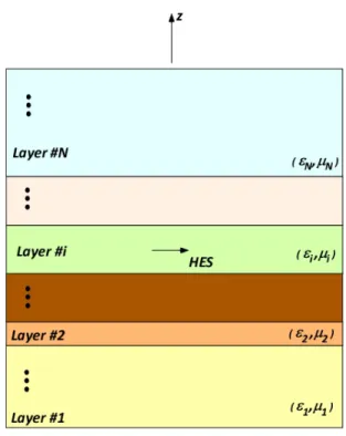
Consider a general layered medium with a Horizontal Electric Source (HES) belonging to layer i (Fig. 1.8).

(15)

(

)

(

)

{

(

)

}

(

)

{

(

)

}

(

)

( )

{

(

)

}

(

)

( )

{

(

)

}

(

)

{

(

)

}

(

)

{

(

)

}

0 0 1 1 0 0 , | ' , | ' , | ' , | ' , | ' , | ' , | ' . , | ' , | ' , | ' , | ' , | ' , | ' A A A xx yy vv A A zz zz A A zx zu A A zy zu G z z G z z S G k z z G z z S G k z z G z z jcos S G k z z G z z jsin S G k z z K z z S K k z z C z z S C k z z ρ ρ ρ ρ φ φ ρ φ φ ρ ρ ρ ρ ρ ϕ ρ ϕ ρ ρ = = = = − = − = =       (1.44)

Since the outmost layers are semi-infinite media, the spectral domain DGFs are characterized by two branch-point singularities, specifically at kρ = k1 and kρ = kN-1 [6], that are the wavenumber in the first and Nth layer

where the radiation condition has to be satisfied. In addition to the branch-point singularities, there are some Surface Wave Poles (SWPs) located between the minimum and the maximum wavenumber involved in the geometry. The number of SWPs is determined by the dielectric thicknesses and the relative dielectric constants of the media (Fig. 1.9). Therefore, in order to avoid the previous mentioned singularities and guarantee high numerical stability is necessary to deform the Sommerfeld Integration Path (SIP) respect to real axis as shown in Fig. 1.10.

(16)

Figure 1.10. Distortion of the Sommerfeld Integration Path.

The Sommerfeld Integral reported in (1.42) cannot be evaluated analytically except for some special cases. Moreover, the SI numerical solution is very time-consuming due the high-oscillatory and slow-decaying nature of the Bessel functions (Fig. 1.11) even using proper techniques like waiting averages and continued fraction expansions [6]-[11].

-0,5 0 0,5 1 0 5 10 15 20 25 30 J 0 J 1 J 2 Be s s e l F u nc ti o n( x ) x

(17)

Therefore, many recent effort to accelerate the SI computation has been presented in literature and among them the Discrete Complex Image Method (DCIM) is particularly appealing [12]-[17]. The DCIM takes advantage from the fact that if the spectral domain DGFs is approximated in terms of complex exponentials, the analytical evaluation of the SI becomes possible via the Sommerfeld Identity:

( )

0 0 , z i jk z jk r z e e j J k k dk r ρρ ρ k ρ ∞ − − =

∫

(1.45)

where ki is the wavenumber in the dielectric which hosts the source point.

Physically, each exponential term represents a source image with a complex amplitude and location (Fig. 1.12). Therefore the crucial step in the derivation of the closed-form DGFs is the exponential representation of its spectral domain counterpart. The approximation technique which has been employed is the Generalized Pencil Of Functions which results quite reliable and numerical efficient [5] (Appendix B).

Figure 1.12. Real HES with complex images for a typical layered medium.

Since the GPOF method requires a uniform sampling approach along a real variable of a complex function, the SIP must be deformed mapping a

(18)

real variable onto the kz plane [18]. In order to alleviate in advance the

Green’s function investigation and the difficulties generated by the tradeoff between sampling range and sampling period, the approximation is performed in two levels (Fig. 1.13) [18]-[19] The first part of the approximation is carried out along the path Cap1 where the functions are

characterized by a smooth behavior and the second one along the path Cap2 where the DGFs present rapid transitions. The parametric equations

describing the first and second path are:

[

]

1 02 01 2 02 02 : 0 , : 1 0 ap zi i ap zi i C k jk T t t T t C k k jt t T T = − + ≤ ≤    = _− + −_ __ ≤ ≤      (1.46)

where t is the running variable sampled uniformly.

The T02 value is chosen such that kρmax2= k1+T022 ≥kmax, where kmax

is the maximum wavenumber involved in the geometry. On the contrary, the parameter T01 is not critical as long as kρmax1=k T012 +T022 is large

enough to capture the spectral domain DGFs behavior for large value of kρ

where is not necessary to deal with a large number of samples.

Figure 1.13. Definition of the SIP for the two-level approach.

Before performing the approximation in the second region, the approximated function in the first path has been subtracted from the original spectral domain DGFs. The resulting function will be non zero over

(19)

a small range of kρ so one can pick up its fine features without employing a

large number of samples. To make the spectral domain DGFs fast convergent to zero for large value of kρ, the quasi static term ψQS has been

extracted from the function to be approximated:

( )

.

QS k

lim_ρ k_ρ

ψ = →∞ψ (1.47)

The final expressions for the spectral DGFs in the first and second path are reported below:

( )

1 1 1 1 1 02 1 1 1 1 1 1 1 1 1 : , , n z n i i n N N k t ap n n n n jk T n n n n i C k b e a e b a b e jk α β ρ α ξ α − = = − = = = =

∑

(1.48)

( )

(

)

2 2 2 2 2 2 2 2 1 1 2 02 2 2 2 02 : , , 1 n z n i i n N N k t QS ap n n n n k n n n n i C k k b e a e b T a b e k jT α β ρ ρ α ψ ψ ξ α − = = − − = = = = +

∑

(1.49)

where N1,2 are the number of employed exponentials chosen by using a

Singular Value Decomposition (SVD) algorithm, while b1,2n and β1,2n are the

coefficients and exponents obtained via the GPOF method. Since the approximated DGFs must be an exponential representation in terms of kzi,

it is necessary to transform the GPOF coefficients and exponents into a form suitable for the application of the Sommerfeld Identity (a1,2n, α1,2n).

By following the described procedure the DGFs in the wavenumber domain can be express as:

( )

1 2 1 2 1 2 1 1 1 . 2 n zi n zi i N N k k QS n n n n z k a e a e jk α α ρ ψ ψ − − = =   = _ + + _ 

∑

 (1.50)

The spatial domain DGFs f(ρ,z|z’) can be cast in a closed form by substituting the derived approximation forms into the SI and exploiting the (1.45):

(20)

(

)

1 1 2 2 1 2 1 1 1 2 2 2 2 2 1 1 2 2 , | ' . , i i n i n jk N jk r N jk r QS n n n n n n n n n n e e e f z z a a r r r r ρ ρ ψ ρ ρ α ρ α − − − = = = + + = − = −

∑

(1.51)

To demonstrate the effectiveness and the numerical efficiency of the DCIM, the geometries shown in Figs. 1.14-1.15 at the operating frequency of 1.0 GHz have been analyzed.

Figure 1.14. Three-layer structure with an embedded HES.

Figure 1.15. Four-layer structure with an embedded HES.

The chosen approximation parameters for the first and the second complex path are reported in Tab 1.1-1.4 respectively:

(21)

Table 1.1. Approximation parameters for the path Cap1 relative to the example

reported in Fig. 1.14

Dyadic Term T01 # Samples # Exponentials

Gvv 200 100 6

Kφ 200 100 7

Table 1.2 Approximation parameters for the path Cap2 relative to the example

reported in Fig. 1.14.

Gvv 0.345 100 12

Kφ _0.345 ₁₀₀ ₁₄

Gvv 200 100 8

Kφ 200 100 11

Gvv 1.34 100 11

(22)

The spectral DGF elements Gvv and K

φ

 and their exponential approximations have been reported in Figs. 1.16-1.23.

-0.1 0 0.1 0.2 0.3 0.4 0.5 0 30 60 90 120 150 180 0 1000 2000 3000 4000 5000 6000 Data Approx Exact Approximation M ag ni tud e P h as e( deg ree s ) k_ρ Phase Magnitude

Figure 1.16. Exponential approximation for the term Gvvin the path Cap1 for the

example reported in Fig. 1.14.

-0.2 -0.1 0 0.1 0.2 0.3 0.4 0 30 60 90 120 150 180 0 1000 2000 3000 4000 5000 6000 Data Approx Exact Approximation M ag ni tu d e P h as e( deg ree s ) k_ρ Phase Magnitude

Figure 1.17. Exponential approximation for the term Kφ in the path Cap1 for the

(23)

0 5 10-5 10-4 1,5 10-4 2 10-4 -60 0 60 120 180 0 5 10 15 20 25 30 B B Exact Approximation M ag ni tu d e P h as e( deg ree s ) k_ρ Phase Magnitude

Figure 1.18. Exponential approximation for the term Gvv in the path Cap2 for the

example reported in Fig. 1.14.

-10-4 0 10-4 2 10-4 0 60 120 180 5 10 15 20 25 30 Data SI Exact Approximation M ag ni tud e P h as e( deg ree s ) k ρ Phase Magnitude

Figure 1.19. Exponential approximation for the term Kφ in the path Cap2 for the

(24)

-0,1 0 0,1 0,2 0,3 0,4 0,5 0 30 60 90 120 150 180 0 1000 2000 3000 4000 5000 6000 Data Approx Exact Approximation M ag ni tu d e P h as e( deg ree s ) k_ρ Phase Magnitude

Figure 1.20. Exponential approximation for the term Gvvin the path Cap1 for the

-0.09 -0.045 0 0.045 0.09 0.135 0.18 -180 -120 -60 0 60 120 180 0 1000 2000 3000 4000 5000 6000 Data Approx Exact Approximation M ag ni tud e P h as e( deg ree s ) k ρ Phase Magnitude

(25)

-1 10-5 0 1 10-5 2 10-5 3 10-5 4 10-5 5 10-5 -180 -120 -60 0 60 120 180 0 10 20 30 40 50 Data Approx Exact Approximation M ag ni tu d e P h as e( deg ree s ) k ρ Phase Magnitude

Figure 1.22. Exponential approximation for the term Gvv in the path Cap2 for the

-9 10-5 -6 10-5 -3 10-5 0 3 10-5 6 10-5 9 10-5 -180 -120 -60 0 60 120 180 10 20 30 40 50 Data Approx Exact Approximation M ag ni tud e P h as e( deg ree s ) k ρ Phase Magnitude

(26)

The related closed form DGFs in the spatial domain are presented in Figs. 1.24-1.27 and compared with the numerical solution of the SI.

-6 -4,5 -3 -1,5 0 1,5 3 -180 -120 -60 0 60 120 180 -3 -2 -1 0 1 DCIM SI DCIM SI Log 10 (4 πG x x ) P h as e( G x x ₎ Log 10(k0ρ) Phase Magnitude

Figure 1.24. Magnitude and phase for the vector potential Gxx relative to the

-6 -4,5 -3 -1,5 0 1,5 3 -180 -120 -60 0 60 120 180 -3 -2,5 -2 -1,5 -1 -0,5 0 0,5 1 DCIM SI DCIM SI Lo g 10 (4 πK φ ) P_h as e( K φ ) Log 10(k0ρ) Phase Magnitude

Figure 1.25. Magnitude and phase for the scalar potential Kφ_{relative to the}

(27)

-6 -4,5 -3 -1,5 0 1,5 3 -180 -120 -60 0 60 120 180 -3 -2 -1 0 1 DCIM SI DCIM SI Log 10 (4 πG x x ) P h as e( G x x ₎ Log 10(k0ρ) Phase Magnitude

Figure 1.26. Magnitude and phase for the vector potential Gxx relative to the

example reported in Fig. 1.15.

-6 -4,5 -3 -1,5 0 1,5 3 -180 -120 -60 0 60 120 180 -3 -2 -1 0 1 DCIM SI DCIM SI Lo g 10 (4 πK φ ) P_has e( K φ ) Log 10(k0ρ) Phase Magnitude

Figure 1.27. Magnitude and phase for the scalar potential Kφ relative to the example reported in Fig. 1.15.

(28)

It is evident that the agreement between the exact (SI) and the approximated data (DCIM) remains extremely good in all the analyzed cases.

After the introduction of the proposed method, there have been a plenty of discussions and improvements on the technique. The discussions have concentrated mainly on the approximation procedure since it provides accurate results for horizontal distanced as far as k0ρ ≈20-30 and

beyond they start to deteriorate significantly. The SWP contribution, which is not considered in the proposed method, is the responsible for the violent degradation of the approximation accuracy. In [19] Aksun at alt. have tried to take into account the SWPs in terms of complex images without obtaining a significant improvement of the DCIM accuracy for large value of the ρ. The deterioration is mainly due to the incompatible nature of the approximating functions which are spherical waves (complex images) and the approximated functions which are cylindrical waves (surface waves) [19]. To eliminate this inherent problem, the SWPs must be subtracted from the spectral DGFs before the approximation and their contribution added after the procedure. This approach, when used in conjunction with the DCIM, eliminates all the problems in casting the Green’s functions in closed-forms for all the distance between source and observation points. Although finding the SWPs and the associated residues at the frequency of interest is quite easy and robust [20], keeping all the complex images in the implementation of the MoM procedure for large problems can become computationally very expensive. Since the Green’s functions behave exactly like the SWP contribution after a certain threshold [16], using the DCIM approach beyond a certain distance without extracting the SWPs and using only the SWP terms after the threshold can be sufficient. The evaluation of the switching limit can be easily accomplished adaptively during the calculation of the MoM matrix entries.