3.1 Introduction 3 Simulations

3 Simulations

3.1 Introduction

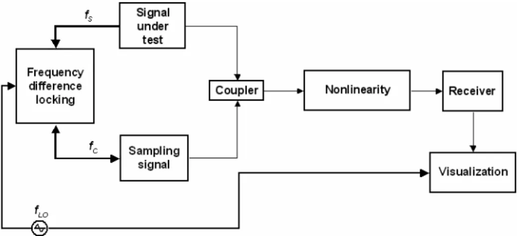
To understand how the Quasi-Asynchronous (Fig. 3.1) optical sampler works, its behavior has been simulated through a Matlab script.

Fig. 3.1: General scheme of the Quasi-Asynchronous sampler.

The working principle (which will be explained in a more detailed way in the next chapter) of the Quasi-Asynchronous sampler is shown in Figure 3.1. The sampler simulated in this chapter is based on nonlinear interaction (polarization rotation induced by XPM) in optical fiber between the signal to be resolved and a sampling ultra-short pulse train whose frequencies are locked to a fixed difference by a nonstandard PLL

circuit. The frequency mismatch leads to a relative shift of the sampling signal on the signal under test (Fig. 3.2) in the time domain.

The FWHM (Full Width Half Maximum) of the sampling pulse and of the signal pulse are given as program input. We have also defined a variable ∆T which represents the difference between the the sampling signal period and the signal under test period, and it is responsible of the system resolution (Fig. 3.2):

C S

T T T

∆ = − [sec] (3.1)

More in general it is possible to say that: 1 c s N T f f ∆ = − (3.2)

where N is the number of bits of the pattern to be visualized. So: s c c s f Nf T f f − ∆ = (3.3)

With the PLL scheme we lock the frequency mismatch to a fixed value fLO:

LO S C

f = f N− f [Hz] (3.4)

The samples frequency at the receiver is still fC, but exploiting a slow photodiode (PD) we are able to correctly reconstruct the envelop of the samples train that represents the acquired signal, with a new period equal to fLO (1/fLO is the acquisition time of this kind of sampler). It means the signal undergoes a time rescaling from a period N/fS to a period 1/fLO.

The frequency fLO is also used to trigger the oscilloscope, as shown in Figure 3.1 where the block “Frequency difference locking” is assumed to be a nonstandard PLL.

and this is the reason why the resolution (Fig. 3.2) depends on the variable ∆T. TS TC Signal under test Sampling signal t t t0 t1 ti

Fig. 3.2: Quasi-Asynchronous sampling operation.

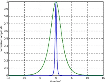
In the following simulations, it is chosen for simplicity N=1 (i.e. acquiring not a bit pattern but just a pulse), so the pattern period corresponds to the bit period; both the sampling pulse and the signal under test are molded as sech2 pulses as it is possible to see in Figure 3.3. -15 -10 -5 0 5 10 15 0 0.1 0.2 0.3 0.4 0.5 0.6 0.7 0.8 0.9 1 time [ps] nor m a li z ed am pl it ud e

The nonlinear effect on which the simulated sampling operation is based is polarization rotation induced by XPM, where the sampling signal acts as the pump and the phase shift induced on the signal under test turns directly in a polarization rotation. The efficiency of the effect is defined as

2 2 b η_{= ⎜}⎛ ⎞_⎟ ⎝ ⎠ (3.6) or 2 2 a η_{= ⎜}⎛ ⎞_⎟ ⎝ ⎠ (3.7)

depending on the fact that the phase shift ΦNL, defined as

(3.8)

( )

( )

( )

( )

( )

∑

is smaller or bigger than π/2 respectively. In (3.8) P(t) is the signal instant power,

γ is the fiber nonlinear coefficient, Leff is the effective length of the fiber and N is the

number of channels.

The factors a and b are

( ) ( ) (

)

1 2cos sin cos NL

a= + θ θ Φ (3.9)

( ) ( ) (

)

1 2 cos sin cos _NL

b= − θ θ Φ (3.10) where θ is

(

)

(

)

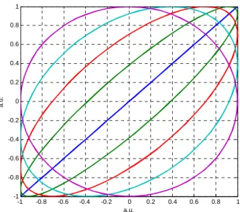
In the following picture it is shown how signals polarization state changes from linear to circular depending on the value of ΦNL (from 0° to 90°).

-1 -0.8 -0.6 -0.4 -0.2 0 0.2 0.4 0.6 0.8 1 -1 -0.8 -0.6 -0.4 -0.2 0 0.2 0.4 0.6 0.8 1 a.u. a. u.

Fig. 3.4: Polarization state (with a fiber length of 2km) changing the value of ΦNL.

3.2 Simulations results

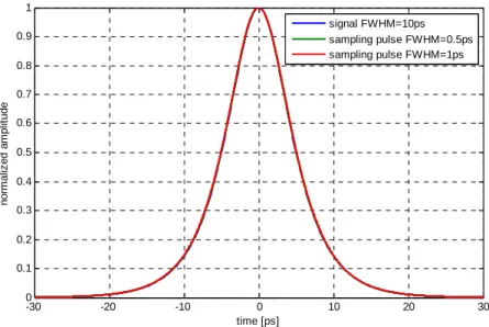
One of the crucial features for a good sampler or a sampling oscilloscope is the resolution. For the Quasi-Asynchronous optical sampler, resolution is mainly related to the sampling pulsewidth and to the ∆T defined in (3.1)-(3.2). In the next simulation results it is shown a comparison between the input signal (a pulse in this case) and the traces acquired by the Quasi-Asynchronous optical sampler, fixing ∆T equal to 250fs, for different sampling pulse FWHM (1 and 0.5ps) and different signal pulse FWHM (10–5–2–1ps).

Comparing, for example, Figure 3.5 and 3.7 it is possible to notice that, when the signal pulse FWHM is comparable with the sampling pulse FWHM, the acquired signal enlarges itself in respect of the original pulse. However in Figure 3.8 a signal pulse with a FWHM of 1ps is sampled with a sampling pulse with the same FWHM, and even if the acquired signal is a little more wide than the original signal, it is possible to appreciate the fact that the signal shape is perfectly reconstructed.

-30 -20 -10 0 10 20 30 0 0.1 0.2 0.3 0.4 0.5 0.6 0.7 0.8 0.9 1 time [ps] no rm a liz ed am pl it u d e signal FWHM=10ps sampling pulse FWHM=0.5ps sampling pulse FWHM=1ps

Fig. 3.5: Simulation results with a signal pulse FWHM of 10ps.

-20 -15 -10 -5 0 5 10 15 20 0 0.1 0.2 0.3 0.4 0.5 0.6 0.7 0.8 0.9 1 time [ps] nor m a liz e d am pl it ude signal FWHM=5ps sampling pulse FWHM=0.5ps sampling pulse FWHM=1ps

-10 -8 -6 -4 -2 0 2 4 6 8 10 0 0.1 0.2 0.3 0.4 0.5 0.6 0.7 0.8 0.9 1 time [ps] n o rm al iz ed am pl it ude signal FWHM=2ps sampling pulse FWHM=0.5ps sampling pulse FWHM=1ps

Fig.3.7: Simulation results with a signal pulse FWHM of 2ps.

-5 -4 -3 -2 -1 0 1 2 3 4 5 0 0.1 0.2 0.3 0.4 0.5 0.6 0.7 0.8 0.9 1 time [ps] nor m a liz ed a m pl it ude signal FWHM=1ps sampling pulse FWHM=0.5ps sampling pulse FWHM=1ps

Fig.3.8: Simulation results with a signal pulse FWHM of 1ps.

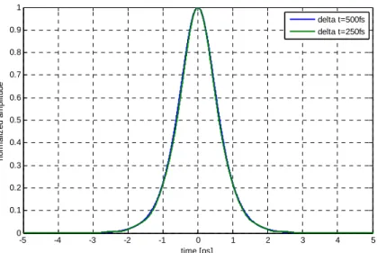
The impact of the choice of ∆T value on the resolution limitation is much less decisive than the sampling pulsewidth. In fact it is not a problem to experimentally obtain a ∆T value of 500 or 250fs, but as shown in Figures 3.9 and 3.10, the acquired signals in the two different cases basically fit together, even reconstructing a 1ps-signal pulse.

-5 -4 -3 -2 -1 0 1 2 3 4 5 0 0.1 0.2 0.3 0.4 0.5 0.6 0.7 0.8 0.9 1 time [ps] no rm al iz ed am p lit ude delta t=500fs delta t=250fs

Fig. 3.9: Acquired signals in the case where the signal pulse FWHM and the sampling pulse FWHM are equal to 1ps

and 0.5ps respectively. -20 -15 -10 -5 0 5 10 15 20 0 0.1 0.2 0.3 0.4 0.5 0.6 0.7 0.8 0.9 1 time [ps] norm a liz ed am pl it ude delta t=500fs delta t=250fs

Fig. 3.10: Acquired signals in the case where the signal pulse FWHM and the sampling pulse FWHM are equal to

5ps and 0.5ps respectively.

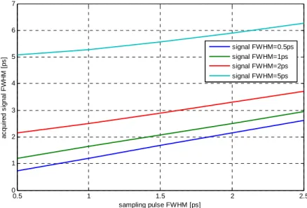
In Figure 3.11 and 3.12 the enlargement of the acquired signal width with the growth of the sampling pulse FWHM is reported.

0.5 1 1.5 2 2.5 0 1 2 3 4 5 6 7 sampling pulse FWHM [ps] ac qui red s ignal F W H M [ p s ] signal FWHM=0.5ps signal FWHM=1ps signal FWHM=2ps signal FWHM=5ps

Fig. 3.11: Acquired signal FWHM versus sampling pulse FWHM for different values of the original signal width

with ∆T=250fs. 0.5 1 1.5 2 2.5 0 1 2 3 4 5 6 7 sampling pulse FWHM [ps] ac qui red s ignal F W H M [ p s ] signal FWHM=0.5ps signal FWHM=1ps signal FWHM=2ps signal FWHM=5ps

Fig. 3.12: Acquired signal FWHM versus sampling pulse FWHM for different values of the original signal width

with ∆T=500fs.

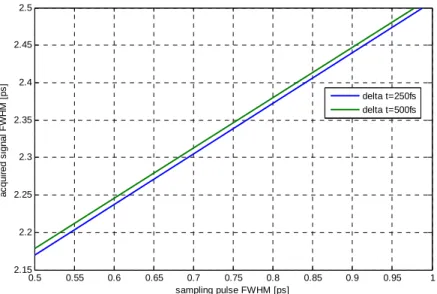
This two pictures are reported for two different values of ∆T; in this case it is possible to notice the slight impact of the different resolution on the correct acquisition of the signal, (as shown in a better way in Figure 3.13).

0.5 0.55 0.6 0.65 0.7 0.75 0.8 0.85 0.9 0.95 1 2.15 2.2 2.25 2.3 2.35 2.4 2.45 2.5 sampling pulse FWHM [ps] ac qu ir ed s ig nal F W H M [ p s ] delta t=250fs delta t=500fs

Fig. 3.13: Acquired signal FWHM versus sampling pulse FWHM for two different values of ∆T for a signal FWHM

of 2ps.

The importance of keeping short enough the parameter ∆T is reported in Figure 3.14 where it is possible to notice that for signal pulsewidth large enough (3ps, 4ps and 5ps) versus sampling pulse width the effect of the growth of ∆T is a little enlargement of the acquired signal width. Instead for signal pulsewidths which are comparable with the sampling pulse width we have a sort of quantization error (red and blue lines in Figure 3.14) because the resolution is not precise enough to correctly visualize such narrow signals. 1 1.5 2 2.5 3 3.5 4 4.5 5 5.5 ac qu ir ed s ign al F W H M [ p s ] signal FWHM=0.5ps signal FWHM=1ps signal FWHM=2ps signal FWHM=3ps signal FWHM=4ps signal FWHM=5ps

In the Matlab script it is also calculated a percentage error ε which shows the enlargement of the acquired signal width among the original signal width:

100 ⎛ − ⎞ = ⎜⎜_⎝ acq sign _⎠ sign FWHM FWHM FWHM ε _⎟⎟× (3.12)

In Figure 3.15 it is possible to see again the quantization error which depends on the system resolution.

300 400 500 600 700 800 900 1000 0 20 40 60 80 100 120 140 160 180 200 delta t (fs) err o r (% ) signal FWHM=0.5ps signal FWHM=1ps signal FWHM=2ps signal FWHM=5ps

Fig. 3.15: Percentage error versus ∆T.

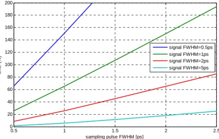
In the next two pictures there are two graphs of ε for two different values of ∆T versus the sampling pulse width.

0.5 1 1.5 2 2.5 0 20 40 60 80 100 120 140 160 180 200 sampling pulse FWHM [ps] e rro r (% ) signal FWHM=0.5ps signal FWHM=1ps signal FWHM=2ps signal FWHM=5ps

Fig. 3.16: Percentage error versus sampling pulse FWHM for ∆T=250fs.

0.5 1 1.5 2 2.5 0 20 40 60 80 100 120 140 160 180 200 sampling pulse FWHM [ps] er ror (% ) signal FWHM=0.5ps signal FWHM=1ps signal FWHM=2ps signal FWHM=5ps

Fig. 3.17: Percentage error versus sampling pulse FWHM for ∆T=500fs.

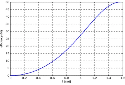
In the following picture the XPM efficiency is reported considering a signal power of 1mW, and a pump power of 4mW. In Figure 3.18 it is possible to see how the efficiency changes with the phase shift ΦNL, whereas in Figure 3.19 it is reported the efficiency growth versus the fiber length.

0 0.2 0.4 0.6 0.8 1 1.2 1.4 1.6 0 5 10 15 20 25 30 35 40 45 50 fi [rad] e ff ici e n cy ( % ) Fig. 3.18: η versus ΦNL. 0 1 2 3 4 5 6 0 5 10 15 20 25 30 35 40 45 50 e ffic ie n c y ( % ) L fiber [Km]