CHAPTER 3
FINANCIAL FRICTIONS, ASSET
PRICES AND MONETARY POLICY
IN THE EURO AREA
1
INTRODUCTION
What does the relevance of the financial frictions in the Euro Area imply for monetary policy? This is the question I want to address in this chapter. On the one hand this means to answer the more detailed question: which is the optimal monetary policy (in the form of an optimal state contingent rule), given that the model of the Euro Area economy is the one estimated in the previous chapter? On the other hand, since I am interested also in deriving policy suggestions for the monetary authority, and given the fact that the optimal policy is often difficult1 to implement, I would also focus on some simple monetary rules, in
their form of the Taylor rule or of an augmented Taylor rule, and on their impli-cations for the monetary policy objectives if adopted. This would mean answer the further questions: what does the presence of the credit market variables or of asset prices imply for monetary policy? Should the monetary authority respond to them? If so, how and in what extent?
In order to pursue these aims, I will implement two types of monetary policy exercises. Both of them want to evaluate the performance of different policy rules in terms of the loss experimented by the Central Bank in adopting them. The difference lays in the fact that on one hand the policy rules are simple ad hoc rules, whose response coefficients are imposed a priori, and on the other hand the rules are the state contingent ones.
The aims and the main original contributions of these paper are three. First, deriving the optimal state contingent rule given an estimated model for the Euro Area which incorporates several frictions, among which the most important are the financial ones.
Second, shed some light in the still controversial issue of whether it is useful or not to target2 the asset prices, evaluating the Euro Area experience.
Third, the most important, answer to the question: does it make sense to target variables which are proxies of the credit markets conditions, such as the financial premium?
The paper is developed as follows. In the first section I will derive the optimal state contingent monetary policy rules (one for each set of central bank’s preferences about the different objectives), solving the minimization problem of the central bank, and I will compute the losses implied by each rule. In the
1See the section ”SIMPLE RULE” for an explanation of this difficulty.
2The meaning of the word ”target” may be misleading. In this context it means that the
monetary authority react to them is some way, or in other words the they are in the interest rate rule. It does not then mean that the monetary authority has asset prices as an argument of its objective function.
second section I will evaluate the performances of some simple ad-hoc monetary rules, focusing on the Taylor rule and on some Taylor type rules, both in their forward and backward looking versions. Before the concluding remarks, I will evaluate the desirability and the extent to which the Central Bank should target the assets prices or the financial premium.
2
STATE CONTINGENT RULES
The minimization problem that the Central Bank has to solve in order to derive a state contingent rule is nothing more that an optimal regulator problem. I already explained in the first chapter the meaning of this kind of problems.
The objective function is the same as in that chapter, and this implies that it has the same convergence properties. Nevertheless, the constraint now is represented by the model estimated in the second chapter3. This fact obliges
me to spend some words in explaining the procedure to derive the monetary rule that, given the nature of the constraint, is different from the case in which the constraint does not deals with rational expectations. Moreover, differently from the first chapter, here I am not going to use the dynamic programming method but the Lagrangian one.
The minimization problem is the following
max {brn t} E0 ∞ X t=0 βt{X0 tRXt+ 2brtnW Xt+ brn0t Qbrtn} (1) s.t. A+EtXt+1+ A0Xt+ A−Xt−1+ Bbrnt + Cet= 0
where Xtis a 22x1 vector of endogenous variables
Xt= ³ b ctbltdbt dinvt bqtbktnwct brtkbrtybtw/pdtmcctbπtzbt bst bat bxtεbβt bεLt bπtεbRt bgt ´0 where4 db
t ≡ brnt − brt−1n and et is a 7x1 vector of innovations identically
and independently distributed with zero mean and variance-covariance Σe. The
matrices A+, A0, A−and C are matrices5containing the model’s parameters and
referring to the forward looking, contemporaneous and predeterminate variables respectively. B is a 22x1 vector. R, W and Q are matrices which select the relevant variables from the vector Xt(inflation, output and the nominal interest
rate first differences).
Before writing the Lagrangian equation, I re-write the above system of equa-tions in matrix form in order to solve it later in the text. The matrix form is the following £ A+ 0 ¤·EtXt+1 Etrbt+1n ¸ +£A0 B ¤·Xt b rn t ¸ +£A− 0 ¤·Xt−1 b rn t−1 ¸ + Cet= 0 3The model which I refer to is the log linearized one presented in the second chapter’s
section called ”General Equilibrium”.
4In the estimated model there was not the variable bd
t, but adding it does not change the
nature of the problem given that it is defined as an identity, so it is not a new equation.
This manipulation allows me to write the objective function (equation 1) as follows 1 2 ∞ X t=0 βtZ0 tV Zt where Zt= [Xt brnt] and V= µ R W W0 Q 
The Lagrangian of this problem is
L = E0 ∞ X t=0 βt[X0 tRXt+ 2rntW Xt+ brtn0Qrnt] + 2Λ0t[A+EtXt+1+ A0Xt+ A−Xt−1+ Bbrnt + Cet]
The first order conditions are
∂L ∂Xt : 2RXt+ 2W brtn0+ β−1A0+Λt−1+ A00Λt+ βA0−Et(Λt+1) = 0 t = 1, 2, ... ∂L ∂brn t : 2W0X t+ 2Qrn0t + B0Λt= 0 t = 0, 1, 2, ... ∂L ∂Xt : 2RX0+ 2W br n 0 + A00Λ0+ βA0−Et(Λ1) = 0 t = 0 ∂L ∂Λt : A+EtXt+1+ A0Xt+ A−Xt−1+ Bbr n0 t + Cet= 0
This system of equations preserves its recursive nature if and only if6Λ 0= 0
and for given initial values for Xt.
Using the definitions above the first order conditions may be written as
V Zt+ β−1 · A0 + 00 ¸ Λt−1+ · A0 0 B0 ¸ Λt+ β · A0 − 00 ¸ EtΛt+1= 0
with Λ0= 0 and X0 given.
Together with the original system £ A+ 0 ¤ EtZt+1+ £ A0 B ¤ Zt+ £ A− 0 ¤ Zt−1+ Cet= 0
I obtain a new dynamic stochastic equilibrium model augmented by the Lagrangian multipliers. In fact, the first order conditions may be written as
A+ 0 0 0 0 0 0 0 βA0− 0 0 0 0 0 0 0 0 0 0 0 0 I 0 0 0 0 0 0 I 0 0 0 0 0 0 I EtXt+1 Etrt+1n EtΛt+1 Xt b rnt Λt + A0 B 0 A− 0 0 R W A00 0 0 β−1A0+ W Q B0 0 0 0 I 0 0 0 0 0 0 I 0 0 0 0 0 0 I 0 0 0 Xt rnt Λt Xt−1 b rnt−1 Λt−1 + Cet 0 0 0 0 0 = 0 so that
6This open the well known issue of the intertemporal inconsisteny of a pociy based on this
Γ0Yt+ Γ1Yt−1+ Πηt= 0 (2) where Yt= ¡ EtXt+10 Etbrt+1n0 EtΛ0t+1 Xt0 brtn0 Λ0t ¢0 and ηt= (e0t 0 0 0 0 0) 0 . This is indeed just a larger linear rational expectation model that can be solved by the techniques I used in the second chapter. Here it is worth noting that the solution of the above enlarged system has a general solution such that
Jt= bg (Xt−1, Λt−1, et)
where Jt≡ [Xt0 brt0n Λ0t]0and bg is approximation of some order of the decision
rule. In my case the approximation is at the first order, hence the transition rule becomes
Jt= HJt−1+ Get (3)
This last result clearly shows that the optimal policy is directly obtained. In particular, it is easy to see that it depends on the vector of lagged Lagrange multipliers. These Lagrange multipliers enter the rule to ensure that today’s policy validates how private sector expectations were formed in the past.
Given the fact that it should not be clear how a policy rule looks like, I report as an example the rule in the case in which λ=0.5 and ν = 0.2, i.e. the case in which the central bank is inflation oriented but it also moderately cares about both the output stabilization and the gradualism of the the monetary policy. The rule is presented in the next page.
b rn t = −0.006768bqt−1− 0.075413bkt−1+ 0.005874 cnwt−1− 0.00305brt−1+ −0.040789bat−1− 0.145554bxt−1− 0.064289belt−1+ 0.049621bgt−1+ +0.211703brn t−1+ 0.000997Λ (10) t−1− 0.001007Λ (13) t−1 − 0.39324Λ (21) t−1+ +0.16862bct−1+ 0.008924brkt−1+ 0.064462beβt−1− 0.330504Λ (2) t−1+ +0.39324Λ(3)t−1 Λ(2)t = 0.002733bqt−1+ 0.026067bkt−1− 0.002533 cnwt−1+ 0.001315brt−1+ +0.014115bat−1+ 0.060479bxt−1+ 0.020684belt−1− 0.019583bgt−1+ +0.15608brn t−1+ 0.003073Λ (10) t−1 − 0.003104Λ (13) t−1 − 0.47689Λ (21) t−1+ −0.06764bct−1− 0.003847brt−1k − 0.01184beβt−1+ 0.287105Λ (2) t−1+ +0.47689Λ(3)t−1 Λ(3)t = −0.000608bqt−1− 0.005993bkt−1+ 0.000613 cnwt−1− 0.000318brt−1− −0.003082bat−1− 0.020085bxt−1− 0.004328belt−1+ 0.004874bgt−1+ −0.030321brt−1n + 0.000024Λ(10)t−1− 0.000024Λ(13)t−1− 0.744344Λ(21)t−1+ +0.016941bct−1+ 0.000931brkt−1+ 0.001974beβt−1+ 0.069108Λ(2)t−1+ +0.744344Λ(3)t−1 Λ(10)t = −0.024667bqt−1+ 0.108974bkt−1+ 0.016238 cnwt−1− 0.00843brt−1+ +0.062995bat−1+ 0.51043bxt−1+ 0.116382belt−1− 0.000747bgt−1+ −0.000798brn t−1+ 0.999618Λ (10) t−1− 1.009716Λ (13) t−1− 0.002628Λ (21) t−1+ +0.003162bct−1+ 0.024669brkt−1− 0.008431beβt−1+ 0.000401Λ (2) t−1+ +0.002628Λ(3)t−1 Λ(13)t = −0.006052bqt−1− 0.029856bkt−1+ 0.005031 cnwt−1− 0.002612brt−1+ −0.019495bat−1− 0.01714bxt−1− 0.025107belt−1+ 0.027139bgt−1+ −0.208399brn t−1+ 0.00074Λ (10) t−1− 0.000747Λ (13) t−1− 0.277679Λ (21) t−1+ +0.093912bct−1+ 0.007643brt−1k + 0.014941beβt−1− 0.244625Λ (2) t−1+ +0.277679Λ(3)t−1 Λ(21)t = 0
It is clear that the condition that the initial values of the Lagrangian mul-tipliers7 have to be zero is necessary and sufficient to solve the above recursive
system of equations, whose solution gives indeed the optimal state contingent rule.
Before the presentation of the results obtained, I present two useful remarks about the derivation of the loss values. They can be found in Dennis (2005).
Remark 1: let bK ≡
00 R0 W0 0 W0 Q
. Then, using the transition rule 3, the loss function can be written as
Loss (t, ∞) = · J0 t−1H0P HJb t−1+ e0tG0P Geb t+ β 1 − βtr ³ G0P GΣb e ´¸
where P≡ bK + βH0P H (See Appendix A2).b
Remark 2: a consequence of Remark 2 is that lim
β→∞(1 − β) Loss (t, ∞) = tr (V ΣJ)
where ΣJis the unconditional variance-covariance matrix of Jtand V=
µ
R W W0 Q
(See Appendix A3).
2.1
Losses evaluation
In this section I present the losses associated with different optimal state con-tingent rules (one for each set of weights of the loss function), computed as explained in the Remark 2.
I would stress that the period t loss function has the following form
Lt= bπt2+ λby2t+ ν ¡ b rn t − brt−1n ¢2
where all the variables are expressed as percentage deviation from their steady state level. As in the first chapter, λ, ν ≥0 are the weights on output stabilization and interest rate smoothing respectively. As in Svensson (1997), ”strict” inflation targeting refers to the situation where only inflation enters the loss function (λ=ν=0), while flexible inflation targeting allows for other goals variables.8 The weight on inflation is always equal to one, hence for instance a
situation in which λ is equal to 0.5 is perfectly equivalent, in terms of loss, to a situation in which the weight on inflation is two and λ=1. In this analysis, the weight ν can assume only the values 0.2 and 0, corresponding to a care to the interest rate smoothing and to an indifference to that objective respectively.
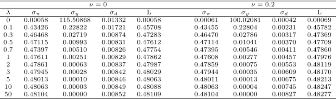
The following table reports the loss values computed as explained in Remark 2.
7The condition on Λ(21)
t is not an a priori initial condition. It comes directly from the
solution of the system in 2.
8It is important to underline this fact because in the literature the expression ”strict
inflation targeting” is often used to indicate the fact that the Central Bank follows a simple monetary rule characterized by the prescription to responde only to inflation. In the same way, with and without smoothing means ν > 0 and ν = 0 respectively, and not the presence of the interest rate lag in the policy rule.
LOSSES OF MODEL WITH FINANCIAL FRICTIONS ν = 0 ν = 0.2 λ σπ σy σd L σπ σy σd L 0 0.00058 115.50868 0.01332 0.00058 0.00061 100.02081 0.00042 0.00069 0.1 0.43426 0.22822 0.01721 0.45708 0.43455 0.22804 0.00231 0.45782 0.3 0.46468 0.02719 0.00874 0.47283 0.46470 0.02786 0.00317 0.47369 0.5 0.47115 0.00993 0.00831 0.47612 0.47114 0.01041 0.00370 0.47709 0.7 0.47397 0.00510 0.00826 0.47754 0.47395 0.00546 0.00411 0.47860 1 0.47611 0.00251 0.00829 0.47862 0.47608 0.00277 0.00457 0.47976 2 0.47861 0.00063 0.00837 0.47987 0.47859 0.00075 0.00553 0.48119 3 0.47945 0.00028 0.00842 0.48029 0.47944 0.00035 0.00609 0.48170 5 0.48013 0.00010 0.00846 0.48063 0.48011 0.00013 0.00675 0.48213 10 0.48063 0.00003 0.00849 0.48088 0.48063 0.00004 0.00745 0.48247 50 0.48104 0.00000 0.00852 0.48109 0.48104 0.00000 0.00827 0.48277
Table 1: All the computed losses are multiplied by 1000. The total loss L is computed as
σπ+λσy+νσr.
In the first place I would stress that having an interest rate smoothing ob-jective implies a higher loss for any given rule, which is totally due to both an increase in the variance of output and to the fact that the interest rate smooth-ing variability is taken into account. Nevertheless, the increase in the total loss is negligible.
Increasing the weight in output (i.e. increasing λ) results in an increase in the total loss. This would suggest that the rule implied by the strict infla-tion targeting regime (λ=0, regardless the presence of interest rate smoothing objective) is the best rule that the Central Bank can adopt.
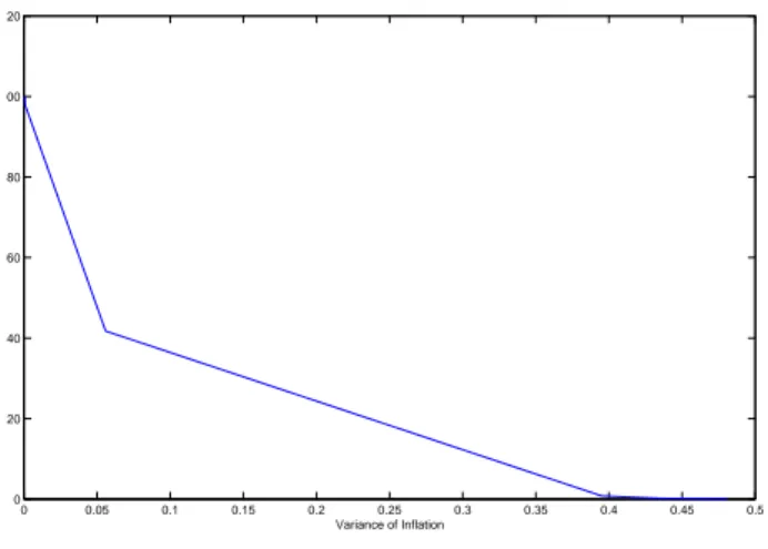
Nevertheless, this rule is most probably not chosen by a Central Bank, for the reason that it seems unlikely that a central bank doesn’t care at all to the variance of the output. It is clear from Figure 1 that a trade-off9exists between
inflation and output variability. Adopting a strict inflation targeting regime would generate a very high output variability, much higher than any other rule. For this reason it seems reasonable to focus on modest weights on output for those central banks which are strongly inflation stabilization oriented.
3
SIMPLE RULES
The rules derived in the previous section have a certain value because (vedi Woodford 2003). Nevertheless, they may not be an easy guide for the policy maker, given their complexity. In fact, the spirit of implementing the monetary policy on the basis of a monetary rule is to have a simple tool that helps the Central bank to implement its policy, together with many other tools usually used.
It is obvious that all the rules I am approaching to study will give a worst macroeconomic result than the optimal rule (the latter is the one that minimizes the loss for a given set of presences parameters). But, for the reason based on the simplicity already explained, it is worth doing such an analysis and trying to answer to the following question: which are the consequences in terms of total losses and variances of the inflation and output, or in other words which is the desirability, of adopting a simple ad-hoc rule instead of the prescribed optimal state contingent rule, given a set of weights for the objective function?
0 0.05 0.1 0.15 0.2 0.25 0.3 0.35 0.4 0.45 0.5 0 20 40 60 80 100 120 Variance of Inflation
Figure 1: Output-inflation efficiency frontier.
Moreover, assuming that the central bank decides to follow a simple rule, which kind of simple rule among the one proposed here guarantees the best macroeconomic performance?
In the analysis I am basically interested in studying simple rules involving responses to inflation (or expected inflation), and in studying the properties of the so called Taylor rule.
Moreover, I want to focus on the response of monetary policy to asset prices and to financial premium. The former issue is largely debated in the literature, but there is not a clear consensus about it. Contrary, the extent and the op-portunity to respond to movements in the financial premium has not been fully studied. I know only two papers dealing with such an issue. One is Faia and Monacelli (2007)10. They use a calibrated (with U.S data) version of the model
with financial accelerator, and they do a welfare analysis of the monetary policy. The other one is Gilchrist and Leahy (2001) who use again the same calibrated model, but they study the opportunity to target the net worth, although they argue that it is the same thing of targeting the financial premium. I will discuss in more detail the main results of both the contributions in the next section.
The rules I am going to consider and compare with the state contingent ones are of the following form:
b rn t = X rjwbt with j=w=π, y, q, S. I will analyze the following rules:
1. a simple Taylor rule (ST), with rπ=1.5 and ry=rq=rS=0
2. the Taylor rule (T), with rπ=1.5, ry=0.5 and rq=rS=0
10They study this issue only in the working paper version of their work dated January 2005.
In the published version dated October 2007 they do not include any analysis of targeting the financial mark up.
3. a simple Taylor rule + asset prices (STA), with rπ=1.5, rq=0.5 and
ry=rS=0
4. a simple Taylor rule + financial premium (STF), with rπ=1.5, rS=0.5 and
ry=rq=0
5. the Taylor rule + asset prices (TA), with rπ=1.5, ry=0.5, rq=0.2 and
rS=0
6. the Taylor rule + financial premium (TF), with rπ=1.5, ry=0.5, rS=0.2
and rq=0.
Moreover, I will consider the forward looking version of those rules, i.e. the same rules with the expected inflation replacing the actual inflation. They are labeled in the same way, but with a lower-case f (forward) before the upper-case T. This because often, different authors (Bernanke and Gertler (1999) among others) choose to study the desirability of targeting asset prices including them in the monetary rule together with the expected inflation, rather than the contemporaneous one in order to take into account their argument that ”the inflation targeting approach ... implies that policy should not respond to changes in asset prices, except in so far as they signal changes in expected inflation”.
3.1
Losses evaluation
In the Table 2 below I report the loss values implied by assuming that the interest rate is set according to a simple rule. I focused only on the case of a Central Bank which wants to stabilize inflation, but it also gives a certain weight to the output stabilization and to the interest rate smoothing, i.e the case λ=0.5 and
ν=0.2. As a consequence, in order to evaluate the desirability of a given simple
rule, I have to compare the losses in Table 2 with the entries of Table 1 of the inflation, output and policy gradualism variances and total loss corresponding to that case, i.e. 0.47114, 0.01041, 0.00370 and 0.47709 respectively.
σπ σy σd L Rel. Loss ST: Simple Taylor (brn t=1.5bπt) 0.01427 139.89346 0.18355 69.99771 146.7 T: Taylor (brn t =1.5bπt+0.5byt) 0.44229 0.48114 0.00375 0.68361 1.4
STA: Simple Taylor + asset prices (brn
t =1.5bπt+0.5bqt) 4.41995 1557.90470 0.00186 783.37267 1641.9
STF: Simple Taylor + financial premium (brn
t =1.5bπt+0.5 bSt) 0.05849 174.78624 0.01560 87.45473 183.3
TA: Taylor + asset prices (brn
t =1.5bπt+0.5byt+0.2bqt) 0.35777 3.68424 0.00330 2.2055 4.6
TF: Taylor + financial premium (brn
t=1.5bπt+0.5byt+0.2 bSt) 0.44235 0.48458 0.00381 0.68540 1.4
Table 2: All the losses are computed assuming λ=0.5 and ν=0.2.
As expected all the rules generate a total variability higher than 0.47709, but the increase in the total loss changes a lot with the rules. To facilitate the comparison, I computed the relative loss (last column of the Table 2), i.e. the ratio between the loss implied by the rule and the loss implied by the optimal rule. In some cases the increase is very high: a simple Taylor rule, for instance,
generates a loss 146 times higher. Things do not improve (rather get worse) adding to it a target for the financial premium, and things degenerate adding a target for the asset prices, with a loss indeed 1642 times higher.
A different story emerges if I consider the performance of the Taylor rule. In fact, the worsening is much less accentuated, stopping the increase to a 1.4 times. A similar result is obtained putting a target for the financial premium. In the end, a Taylor rule augmented with asset prices implies a higher loss, but still acceptable.
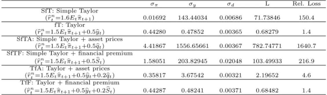
Table 3 reports the results of the same analysis but in the forward looking context. It shows that nothing changes substantially. Hence, I will focus on the simple contemporaneous rules in the rest of the chapter.
σπ σy σd L Rel. Loss SfT: Simple Taylor (brn t=1.6Etbπt+1) 0.01692 143.44034 0.00686 71.73846 150.4 fT: Taylor (brn t=1.5Etbπt+1+0.5byt) 0.44280 0.47852 0.00365 0.68279 1.4
SfTA: Simple Taylor + asset prices (brn
t=1.5Etbπt+1+0.5bqt) 4.41867 1556.65661 0.00367 782.74771 1640.7
SfTF: Simple Taylor + financial premium (brn
t=1.5Etbπt+1+0.5 bSt) 1.58051 203.82945 0.02048 103.49933 216.9
TfA: Taylor + asset prices (brn
t=1.5Etπbt+1+0.5byt+0.2bqt) 0.35817 3.67542 0.00321 2.19652 4.6
TfF: Taylor + financial premium (brn
t=1.5Etπbt+1+0.5byt+0.2 bSt) 0.44287 0.48241 0.00371 0.68482 1.4
Table 3: All the losses are computed assuming λ=0.5 and ν=0.2.
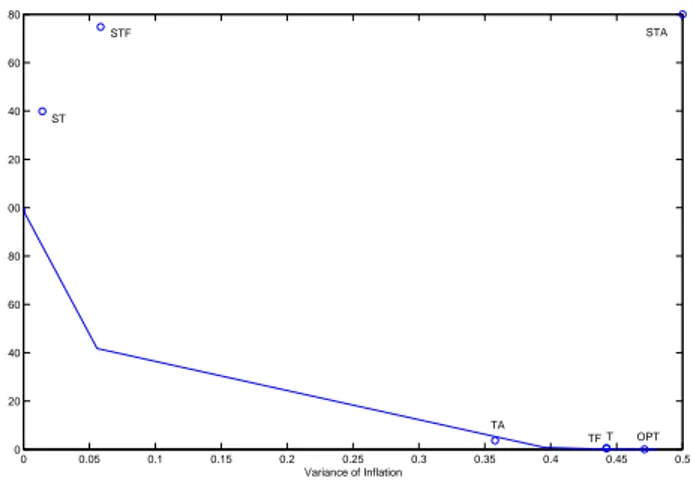
Before doing that, I would compare the simple rules with the optimal one on the basis of the above mentioned output-inflation variability trade-off. In figure 2 I plotted the output-inflation efficiency frontier together with the couple of values of the inflation and output variances implied by the simple rules. The optimal rule is indicated as OPT.
A rule gives a better output-inflation variability combination than the op-timal rule if it stays on the left-lower corner with respect to it. As already explained, there could not be a rule better the the optimal one, but from the figure we can see that while some rules are far away from the optimum, some others are closer.
In particular, the most closer are the ones which we have already seen display an acceptable increase of the total loss, i.e. T, TA and TF. For this reasons, in the next section I will focus on the TA and TF rules to investigate on the asset prices and financial premium targeting regimes.
0 0.05 0.1 0.15 0.2 0.25 0.3 0.35 0.4 0.45 0.5 0 20 40 60 80 100 120 140 160 180 Variance of Inflation ST T OPT TA STA TF STF
Figure 2: Output-inflation efficiency frontier with the variances implied by the simple rules. The point STA does not reflect the true values. I put it in the corner to indicate that it is far away from OPT.
4
MONETARY POLICY ANALYSIS
In the previous section I showed that among the studied simple rules, the Tay-lor rule augmented with either asset prices or with financial premium do not perform bad compared with the Taylor rule (the best one), and they are much better than the other simple rules.
In this section I further investigate the properties of those simple rules. In particular, I will implement other analysis to deepen the issue related to the asset prices and financial premium targeting. Basing my analysis on the TA and TF rules, I will emphasize whether or not it is worth for a central bank responding to asset prices or to the financial premium, which are the optimal response (if any) to those variables given the responses to inflation and output, whether the former should be positive or negative, and what happens to those responses when monetary policy is accommodative (low rπ) rather than aggressive (big
rπ). Part of these questions have already received an (I think not definite)
answer both from a theoretical and an empirical point of view, and using both calibrated and estimated models for different countries (for the U.S. especially). Hence, I am trying also to see whether or not the answers to the mentioned questions hold also for the Euro Area.
4.1
Asset prices
There is not a clear view on the role of asset prices for monetary policy. Two good surveys are Nistico’ (2005) and Gilchrist and Leahy (2001). I do not want to make a new survey here, hence I will report only the most common stances against and pro asset prices targeting.
The most important result I want to refer to is the one derived by Bernanke and Gertler (2001). The main conclusion drawn from the same kind of analysis I am doing here using a calibrated model for the U.S. economy is that for the
purpose of offset inflationary and deflationary pressures, the ”inflation targeting approach dictates that ... policy should not respond to changes in asset prices, except in so far as they signal changes in expected inflation” (p. 78).
The same conclusion is reached by Gilchrist and Leahy (2001) in their liter-ature review. They conclude that ”whereas there are good theoretical grounds for including asset prices in monetary rules, in practice this adds little to sta-bilizing output and inflation. The reason is that asset channels are similar to aggregate demand channels; they tend to increase both output and inflation. Inflation targeting, therefore, yields most of the benefits of asset price targeting without the baggage of the appearance of interfering in the workings of financial markets” (p. 84).
More recently, other studies have shown indeed the contrary. Among others, Cecchetti et al. (2002), Borio and Lowe (2002) and Bordo and Jeanne (2002) argue that central banks can improve macroeconomic performance by reacting to asset price changes. The main argument is that an asset price bubble may lead to excessive growth in investment and consumption, with corresponding fall when the bubble burst. Macroeconomic performance may suffer in terms of excessive variability in output an inflation. A modest tightening or easing of monetary policy when asset prices rise above or below sustainable levels may help smoothing fluctuations in output an inflation11.
What happens then in the Euro Area?
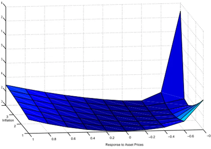
1 2 3 4 −0.8 −0.6 −0.4 −0.2 0 0.2 0.4 0.6 0.8 1 0 0.02 0.04 0.06 0.08 0.1 0.12 0.14
Response to Asset Prices Response to Inflation
Figure 3: Losses deriving from varying the responses to inflation and asset price, with smoothing.
In figure 3 I reported the development of the loss following a variation of both inflation and asset prices, for a given value of the response to output (ry=0.5 in
the picture). In other words, I studied the consequences of contemporaneously varying the mentioned variables adopting a Taylor rule augmented with asset prices targeting.
11Focusing only on output and inflation may not be a good choice to evaluate the desirability
of an asset prices targeting policy. As stressed by Gilchrist and Leahy (2001), there is a dilemma related to the components of output. See next section for further details.
The choice of exploring negative responses to asset prices comes from Faia and Monacelli (2007). As already said, they do a welfare analysis of the mone-tary policy , concluding that ”... the monemone-tary authority [should] lower interest rates when the asset price rises”.12.
The surface is concave and the minimum loss is reached when the response to asset price is around zero, for any given values of rπ.
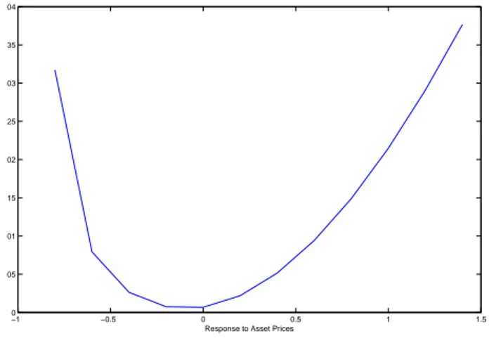
Figure 4 specifies better the optimal responses. It represents a section of the surface in picture 3 for rπ=1.5. It is clear that a value around zero (or slightly
negative) gives the best macroeconomic performance.
−1 −0.5 0 0.5 1 1.5 0 0.005 0.01 0.015 0.02 0.025 0.03 0.035 0.04
Response to Asset Prices
Figure 4: Losses deriving from the variation of the responses to asset price in a the Taylor rule (rπ=1.5, ry=0.5).
I can conclude that in the Euro Area as in the U.S., monetary policy should not target asset prices.
4.2
Financial mark up
The idea of targeting the financial mark-up bears from the fact that if the fi-nancial frictions are relevant for the transmission of monetary policy, amplifying the responses of the real variables to the interest rate shocks, than there may be some room for monetary policy to stabilize inflation and output responding to some measure of those frictions, such as the financial premium.
The idea is not completely new. I already said about the papers dealing with this idea. I want to focus here on Gilchrist and Leahy (2001). The authors use the BGG model (with the same calibration) in order to study the effect of a shock (i.e. a variation) to the entrepreneur net worth. They argue that considering a shock to the financial premium would have had the same meaning. They then evaluate the performance of a simple rule with a target on the net worth. They find that it is very successful in eliminating fluctuations in output if compared with simple inflation targeting rules.
12They argue that ”in [their] context, an increase in the asset price is isomorphic to an
increase in the price of capital relative to consumption goods, and hence acts as an implicit tax on investment.”
Nevertheless, they also find that although it is a rule (as the pure inflation targeting is) that stabilizes output, it does not stabilize the components of output, because rising the interest rate after a net worth shock would act in the direction of reducing investment, but also of reducing consumption (see Figures 9 and 9 in Appendix C). In other words, the central bank should be able to rise the rate faced by investors, without rising the rate faced by consumers. They conclude that this is not a feasible policy, and reacting to asset prices, net worth, or the risk premium does not solve the dilemma.
They suggest that the only thing a central bank can do is to find a balance between the fluctuations of the variables that consumers care about. In order to do it, one can choose any variable in the model as a possible target for the central bank, and ”the best choice will depend on the ability of policy makers to quantify the linkages between observable variables and the distortions in the economy”. This is what I have done in the second chapter, i.e. trying to find those linkages for the Euro Area. In this chapter I am evaluating different simple rules, with a different evaluation criterion, not based on the searching of the balance between fluctuations, but on the evaluation of the relative loss implied by each rule. In other words, knowing that the dilemma exists, what is the best thing that the central bank can do? This exercise is more in line with Bernanke and Gertler (2001).
Before starting the analysis, I would stress that the financial premium changes as a consequence of both a variation in the net worth and in the asset prices. In both cases, an increase of those variables improve the financial conditions of the firm, which in turn reduce the financial premium.
If we are going to find that the central bank should respond to the financial premium (and I will show that this is the case), this would also mean that it should (indirectly) responde to asset prices. This would contrast with the results of the previous section.
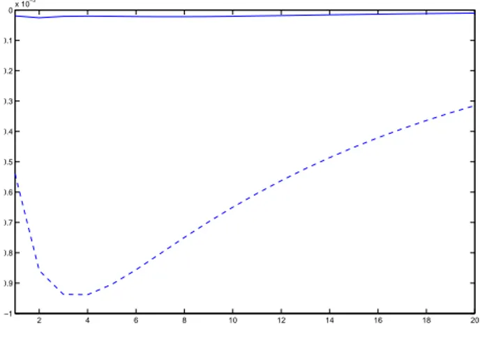
In appendix B I heuristically tried to show that changes in the financial premium are almost completely due to a change in the net worth. Figure 8 highlights that the response of the financial premium is much more big when a shock to the net worth occurs that in the case of an asset prices shock.
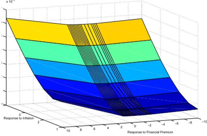
In Figure 5 I reported the result of the same exercise done in the previous sec-tion for the asset prices, i.e. varying inflasec-tion and financial premium responses for a given response to output (always ry=0.5). This analysis highlights that
the optimal response to the financial premium has to be negative. This because the underlining mechanism of the model implies that, when the financial pre-mium is decreasing, the financial conditions of a firm improve, most probably for an increase in the worth, providing more collateral for external debt and, in the end, reducing the cost of external finance and of new investments. If the central bank’s objective is to stabilize inflation and output, it has to increase the interest rate in order to offset the ”unjustified” increase in investment and hence in output, and also to reduce inflation.
This fact appears in a clearer way in Figure 6 where the sections of the surface are reported for different values of inflation. The minimum of the curves always corresponds to a negative value of the coefficient rS.
Another important result emerges. As the monetary policy becomes more and more anti-inflationary, rS becomes more and more negative.
1 2 3 4 −10 −8 −6 −4 −2 0 2 4 6 8 10 0 1 2 3 4 5 6 7 x 10⁻³
Response to Financial Premium Response to Inflation
Figure 5: Losses deriving from varying the responses to inflation and the financial premium, with smoothing. −4 −3 −2 −1 0 1 4.9 5 5.1 5.2x 10 −4
Response to Asset Prices Response to Inflation 1 −4 −3 −2 −1 0 1 6.8 6.9 7 7.1x 10 −4
Response to Asset Prices
Losses Response to Inflation 1.5 −4 −3 −2 −1 0 1 1.24 1.25 1.26 1.27x 10 −3
Response to Asset Prices
Losses Response to Inflation 2 −4 −3 −2 −1 0 1 2.06 2.08 2.1 2.12x 10 −3
Response to Asset Prices Response to Inflation 2.5 −4 −3 −2 −1 0 1 3.08 3.1 3.12 3.14 3.16x 10 −3
Response to Asset Prices
Losses Response to Inflation 3 −4 −3 −2 −1 0 1 4.3 4.32 4.34 4.36x 10 −3
Response to Asset Prices
Losses Response to Inflation 3.5 −4 −3 −2 −1 0 1 5.56 5.58 5.6 5.62 5.64x 10 −3
Response to Asset Prices Respose to Inflation 4
Figure 6: Losses deriving from the variation of the responses to the financial premium in a simple Taylor rule (rπ= 1.5).
4.3
Impulse response functions
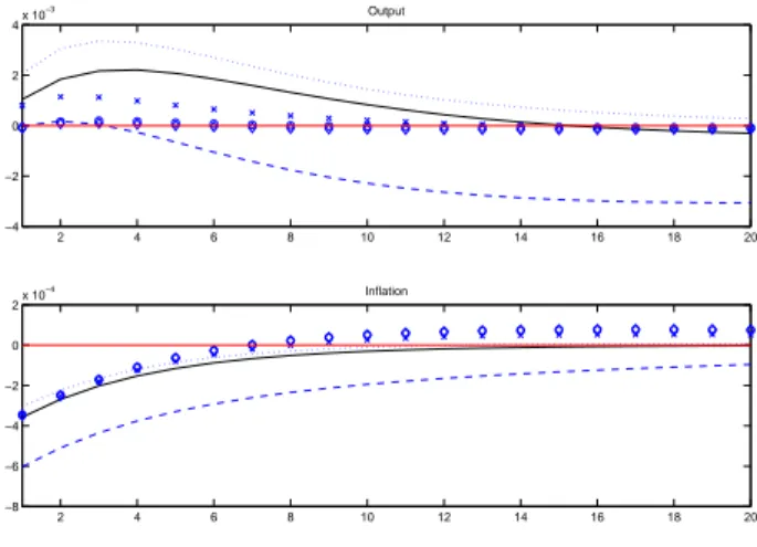
The last exercise I want to implement is related to the analysis of the impulse response functions. In particular, the question is: under which simple rule a technology shock implies less volatility for output and inflation? Or which is the rule that better offset a technology shock?
Figure 7 displays those responses. Output is clearly more stabilized under the Taylor rule (Circled line), the Taylor + Assets prices rule (x-marked line), and the Taylor + Financial Premium rule (diamond-marked line). These per-form much better the the other rules, except the Simple Taylor + Assets prices rule (Dotted line) which gives a similar result (indeed a better one) in the first quarter after the shock. Nevertheless, it seems to imply a very slow return to the equilibrium.
As for inflation, more or less all the rules perform the same, except the Simple Taylor + Assets prices rule.
2 4 6 8 10 12 14 16 18 20 −4 −2 0 2 4x 10 −3 Output 2 4 6 8 10 12 14 16 18 20 −8 −6 −4 −2 0 2x 10 −4 Inflation
Figure 7: Response of Output and Inflation to a technology shock under different simple rules. Simple Taylor: Solid line, Taylor : Circled line, Simple Taylor + Assets prices: Dotted line, Simple Taylor + Financial Premium: Dashed line, Taylor + Assets prices: x-marked line, Taylor + Financial Premium: diamond-marked line.
5
CONCLUDING REMARKS
In this paper I studied the consequences of the relevance the credit market in the Euro Area for monetary policy. After the derivation of the optimal sate contingent rule, I evaluated the properties of some simple ad hoc monetary policy rules. In fact, it is usual to compute the optimal rule and use it as a benchmark. The comparison has been done on the basis of the loss generated by the different rules, but also on the basis of the output-inflation trade-off and on the ability of the rules to offset a technology shock. The main result, common in the literature, is that the Taylor rule is a good simple rule compared with other Taylor type rules. This because it implies an increase of the total loss of only 1.4 times with respect to the optimal rule, it is close to the efficient frontier and it is successful in offsetting a technology shock.
Another important result is that if the Taylor rule is augmented with either a response to asset prices or to the financial premium, these rules perform well. Targeting asset price increases the loss of 4 times, and targeting the financial premium gives very similar results of the Taylor rule. They are also good in terms of nearness to the efficiency frontier and in offsetting the technology shock. Other rules perform definitely worst.
The good performances of the augmented Taylor rule induced me to further investigate their properties. In particular I found that the response to asset prices that minimizes the loss in a Taylor rule is zero (or slightly negative), or in other words it is not optimal for the central bank to target asset prices. As for the financial premium, I found that it is optimal to negatively respond to its variations, with an increasing negative response when monetary policy becomes more anti-inflationary.
References
[1] Akram, Q. Farooq, Brdsen, Gunnar and yvind, Eitrheim (2005),
Monetary Policy and Asset Prices: To Respond or Not?,
Norwe-gian University of Science and Technology Working Paper. [2] Bernanke, Ben and Gertler, Mark (1999), Monetary Policy and
Asset Price Volatility, .
[3] Bernanke, Ben and Gertler, Mark (2001), Should Central Banks Respond to Movements in Asset Prices?, American Economic
Review, 91(2), 253-257.
[4] Bordo, D. G. and Jeanne, O. (2002), Boom - Bust in Asset
Prices, Economic Instability and Monetary Policy, Discussion
Paper 3398, CEPR.
[5] Borio, C. and Lowe, P. (2002), Asset Prices, Financial and
Mon-etary Stability: Exploiting the Nexus, BIS Working Paper No.
114, Basle: BIS.
[6] Cecchetti, G. Stephen, Genberg, Hans and Wadhwani, Sushil (2002), Asset Prices in a Flexible Inflation Targeting Framework, NBER Working Paper No. W8970.
[7] Cecchetti, S. G., Genberg, J. H. and Wadhwani, S. (2000),
As-set Prices and Central Bank Policy, Geneva Reports on the
World Economy 2, International Center for Monetary and Bank-ing Studies and CEPR.
[8] Chadda, J, Sarno, Lucio and Valente, G. (2004), Monetary Policy
Rules, Asset Prices and Exchange Rates, International Monetary
Fund Staff paper, 51, 529-552.
[9] Faia, Ester and Monacelli, Tommaso (2007), Optimal Monetary Policy Rules, Asset Prices and Credit Frictions, Journal of
Eco-nomic Dynamics and Control.
[10] Gilchrist, Simon and Leahy, John V. (2001), Monetary Policy and Asset Prices, Journal of Monetary Economics, 49, 75-97. [11] Issing, Omar (2003), Introductory Statesman at the
ECB Workshop on ”Asset Prices and Monetary Policy”,
http://www.ecb.int/events/pdf/conferences/issing.pdf.
[12] Juillard, Michel and Pelgrin, Florian (2007), Computing Optimal
Policy in a Timeless-Perspective: An Application to a Small-Open Economy, Bank of Canada Working Paper 2007-32.
[13] Nistico’, Salvatore (2005), Stock Prices and Monetary Policy:
Theory and Methods, in Monetary Policy and Institutions, edited
[14] Richard, Dennis (2005), Optimal Policy in Rational Expectations Models: New Solution Algorithms, Federal Reserve Bank of San Francisco Working Paper 2001-09.
[15] Smets, Frank (1997), Financial-asset Prices and Monetary policy: Theory and Evidence.
[16] Svensson, L. E. O. (1997), Inflation targeting: Some Extensions, NBER Working Paper.
[17] Taylor, John (1993), Discretion versus Policy Rules in Practice,
Carnegie-Rochester Conference Series on Public Policy, 39,
195-214.
[18] Woodford, Michael (2000), Pitfalls of Forward-Looking Monetary Policy, American Economic Review, Vol. 90, No. 2, 100-104. [19] Woodford, Michael (2003), Interest and Prices: Foundations of
A
COMPUTATION OF THE LOSS VALUES
A.1
Mathematical preliminary
Assume that 0 < β < 1 and that the spectral radius of the matrix θ is less than one, then the infinite series S =P∞j=0βjθ0j
W θj is convergent. Consequently,
βθSθ = P∞j=0βjθ0j
W θj = S − W , and S can be found as the fixed point of
S=W+βθSθ.
A.2
Establishing Remark 1
Let Jt = XΛtt b rn t and bK ≡ 00 R0 W0 0 W0 Q
. Given the recursive low of motion
Jt= HJt−1+ GetI have Loss (t, ∞) = Et ∞ X t=0 βtJt+j0 V Jt+j (4) = ( Jt0 Ã∞ X t=0 βjH0jV Hj ! Jt+ β 1 − β "∞ X t=0 βjtr ³ G0H10jV H1jGΣe ´#)
which using the result regarding convergent infinite series in Appendix A1 can be simplified to Loss (t, ∞) = J0 tP Jb t+ β 1 − βtr ³ G0P GΣb e ´
where P≡ bK +βH0P H. Finally, again using the law of motion for Jb
tI obtain Loss (t, ∞) = · Jt−10 H0P HJb t−1+ e0tG0P Geb t+ β 1 − βtr ³ G0P GΣb e ´¸ as required.
A.3
Establishing Remark 2
From appendix A2 the loss function can be written as
Loss (t, ∞) = J0 tP Jb t+ β 1 − βtr ³ G0P GΣb e ´ (5)
where P≡ bK + βH0P H, and the economy’s evolution is given byb
Jt= HJt−1+ Get (6)
From equation 6 the unconditional variance-covariance matrix for Jt is the
fixed point of
Using the relations vec(A+B)=vec(A)+vec(B) and vec(ABC)=(C0⊗A)vec(B)
(where vec(A) denotes the vector of stacked column vectors of the matrix A, and
⊗ denotes the Kronecker product) Equation 7 can be solved for ΣJ as follows
vec (ΣJ) = vec (HΣJH0) + vec (GΣeG0) (8)
= (H ⊗ H) vec (ΣJ) + vec (GΣeG0) (9)
Solving for vec(ΣJ) gives
vec (ΣJ) = [I − (H ⊗ H)]−1vec (GΣeG0) Multiplying 5 by (1-β) gives (1 − β) Loss (t, ∞) = (1 − β) Jt0P Jb t+ βtr ³ G0P GΣb e ´ = (1 − β) Jt0P Jb t+ βtr ³ b P GΣeG0 ´
Now employing 7 I have
(1 − β) Loss (t, ∞) = (1 − β) J0 tP Jb t+ βtr h b P (ΣJ− HΣJH0) i = (1 − β) Jt0P Jb t+ βtr ³ b P ΣJ ´ − βtr ³ H0P HΣb J ´ = (1 − β) Jt0P Jb t+ βtr ³ b P ΣJ ´ − tr h³ b P − bK ´ ΣJ i = (1 − β) Jt0P Jb t− (1 − β) tr ³ b P ΣJ ´ + tr ³ b KΣJ ´
Provided the spectral radius of H is less than one, bP will remain bounded
even in the limit as β −→ 1. Therefore, limβ−→∞(1 − β) Loss (t, ∞) = tr
³ b KΣJ ´ . However, defining V= µ R W W0 Q ¶ so that bK ≡ · 0 0 0 V ¸
only the elements in ΣJ
associated with Zt(i.e. Σz) are relevant. Consequently, I have
lim
β−→∞(1 − β) Loss (t, ∞) = tr (V Σz)
B
FINANCIAL PREMIUM RESPONSE
This is an heuristic experiment. I added two (non estimated) exogenous shocks, one to the net worth equation and and the other to the equation of the price of capital. The aim is to study the effects of such a shock on the financial premium. As usual I assumed that both shocks follow a first order autoregressive process with the autoregressive coefficient equal to 0.5 and the variance of innovations equal to to 0.01. 2 4 6 8 10 12 14 16 18 20 −1 −0.9 −0.8 −0.7 −0.6 −0.5 −0.4 −0.3 −0.2 −0.1 0x 10 −3
Figure 8: Response of the financial Premium to a asset prices shock (solid line) and to a net worth shock (dashed line).
C
ASSET PRICES DILEMMA
5 10 15 20 −15 −10 −5 0 5x 10 −4 consumption 5 10 15 20 −4 −2 0 2x 10 −4 labour supply 5 10 15 20 0 2 4 6 8x 10 −3 invesement 5 10 15 20 0 1 2 3 4x 10 −3 asset prices 5 10 15 20 0 0.5 1 1.5x 10 −3 capital 5 10 15 20 0 0.01 0.02 0.03 net worth 5 10 15 20 −2 0 2 4x 10 −3 rk 5 10 15 20 0 0.5 1 1.5x 10 −4 r 5 10 15 20 −2 0 2 4x 10 −4 outputFigure 9: Impulse response functions to a net worth shock.
5 10 15 20 −6 −4 −2 0x 10 −4 mc 5 10 15 20 −1.5 −1 −0.5 0x 10 −4 inflation 5 10 15 20 −2 −1.5 −1 −0.5 0x 10 −3 z 5 10 15 20 −1 −0.8 −0.6 −0.4 −0.2 0x 10 −3 S 5 10 15 20 −15 −10 −5 0 5x 10 −5 rn 5 10 15 20 −6 −4 −2 0 2x 10 −4 wp 5 10 15 20 −4 −2 0 2x 10 −5 d 5 10 15 20 0 0.005 0.01 0.015 enw