2. MOBILITY MODELS

2. MOBILITY MODELS

In the evaluation of wireless networks, simulations are strongly influenced by the mobility model chosen, as shown in [2], [3] and [13]. A model that realistically represents the movement of the nodes is necessary for the study of wireless networks. The use of traces, i.e. mobility patterns observed in real life systems, enables accurate results, especially if the traces describe the behaviour of a large number of users for long observation periods. Unfortunately it is not always possible to collect real life data, in particular when the technology that has to be studied does not exist yet. Besides, even if the statistics can be collected, they are eventually confidential (e.g. due to privacy issues) and then they are not distributed. In these cases it’s necessary to use synthetic models, i.e. algorithms that attempt to mimic the behaviour of the nodes. A variety of synthetic mobility models have been proposed during the years for the study of wireless networks. We can distinguish between two kinds of models: Entity and Group Mobility models.

Next paragraph expounds some of the most important Entity Mobility Models, while the Group Mobility Models are examined in paragraph 2.3.

2.2. ENTITY MOBILITY MODELS

These models emulate the behaviour of the mobile nodes assuming independence between the movements of each other. So, the model can be described considering a single node. The rules that control its movement are then applied to every node independently.

2.2.1. Random Walk

The Random Walk Mobility Model was introduced by Einstein in 1926, and models the movement of the node from the current location to a new one by randomly choosing direction and speed, from the pre-defined range [0,2π] and [vmin,vmax]

respectively. A new couple of values for direction and speed is then calculated after a constant time interval t (Fig. 2.1), or once a constant distance d is travelled (Fig. 2.2). If the node reaches the boundary of the simulation area, it will be absorbed or bounced off. Since the new values do not depend by the previous ones, this model is defined as memory-less.

Fig. 2.1 – Moving pattern of a node using the Random Walk Model (time)

Fig. 2.2 – Moving pattern of a node using the Random Walk Model (distance)

This behaviour results in sudden stops and sharp turns, so it rarely can describe a realistic node movement. Moreover, in [16] Polya proved that, in one and two-dimensional random walk, the probability of return to the origin is certain. For this reason the node tends to move always around its starting point. However, other more complicated mobility models, like the one proposed in [6], make use of it because of its simplicity.

2.2.2. Random Waypoint (RWP)

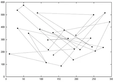
In this model [14] the node alternates periods of movement and pause. It randomly chooses a destination point (waypoint) and moves to it with a constant speed. The speed is uniformly chosen in [Vmin, Vmax]. When the node reaches the destination point, it pauses for a random time and then calculates a new destination and speed. Even this model is then memory-less. An example of RWP is illustrated in Fig. 2.3. Again, this model can rarely describe a realistic movement. Besides, the density of the nodes inside the simulation area is not uniform, as proved in [7]. This effect can compromise the simulation results, as the nodes tend to gather in the centre of the area.

Fig. 2.3 – Moving pattern of a node using the Random Waypoint Model

Fig. 2.4 – Moving pattern of a node using the Random Direction Model

2.2.3. Random Direction

The problem of not uniform density found in the RWP is not present in the Random Direction model [15]. Here, the node moves with a random speed until it reaches the boundary of the simulation region. Then it calculates a new speed and moves in a randomly chosen direction until it reaches the boundary again (Fig. 2.4).

2.2.4. Smooth Random

This model includes the dependences between the previous values of direction and speed with the current ones. In fact the node, moving with a constant speed v, chooses a new random speed value and then accelerates/decelerates until this value is reached [21]. The acceleration value is uniformly distributed between [-amin,amax]. Instead, the direction of the node changes

adding a random value uniformly distributed between [-

θ,θ

Even in this model [17] the old and the new values of speed and direction are correlated. In fact the time is divided into time slots and every

∆

(

)

α

α µ

α

(

)

α

α µ

α

where

α

α

µ

µ

respectively. uk and vk are two independent, uncorrelated and

stationary Gaussian processes with zero means. Fig. 2.5 illustrated an example of the use of this model.

Fig. 2.5 – Moving pattern of a node using the Gaussian-Markov Model

2.2.6. Kinematics

This model simulates the movement of a car on a highway, where the position of the node can be calculated by the changes of acceleration, which depend on the current speed and the driving-control action of the node. At the time interval k, the acceleration is given by:

( )

( ) ( ) ( )

A k = − ⋅a S k +w k +u k

Where S(k) represents the speed, w(k) is a Gaussian process with zero mean, u(k) is the input given by the driver to control the speed, and a represents the reciprocal of the random acceleration-time constant.

2.2.7. City Section

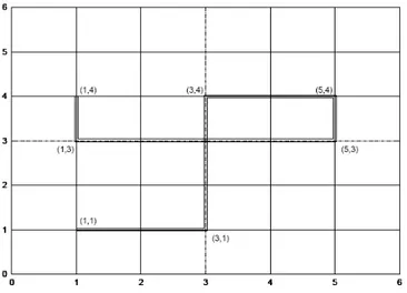
The City Section, or Manhattan [2], model provides realistic movements for a section of a city, where the movement of the nodes is affected by geographical (predefined paths caused by obstacles) and guidelines (traffic laws) factors. In this model the node starts at a defined point at some street and chooses a destination point (Fig. 2.6). Then it travels towards it respecting the traffic laws (one way streets, speed limits, etc.).

Fig. 2.6 – Moving pattern of a node using the City Section Model

The model can be improved including pauses at the intersections (for instance simulating traffic lights), acceleration/deceleration, and variation of concentration in certain sectors (rush hour) and so on [8].

2.2.8. Obstacle

Another model for outdoor environments is the Obstacle Model proposed in [9]. It allows the placement of obstacles in the simulation area, which affects the movement of the nodes and the signal propagation. Once the obstacles (that simulate the presence of buildings in the area) are placed, the model creates a Voronoi diagram [10] using the vertices of the buildings (Fig. 2.7). The nodes will move on this diagram, choosing the destination points and reaching them moving across the shortest path. This model introduces the possibility to add obstacles in the simulation area, but it is good just for outdoor environment and also the movement of the nodes is restricted to the Voronoi graph created.

2.2.9. 3-D Building

This model emulates the movement of an user inside a multi floor building [11]. The node can move horizontally on a floor

bounded by outer walls. It can choose to go forward, back, left or right with a certain probability and moving with a random speed uniformly distributed in [0,Vmax]. The node can also move vertically, but only if it’s in a special region of the floor, called “elevator region”. When the node reaches the elevator region calculates a waiting time or enters in the elevator without a wait. Then it chooses the destination floor. If the node is in the basement, it can also exit from the building (see Fig. 2.8).

2.3. GROUP MOBILITY MODELS

The mobility models described in the previous paragraph represent multiple nodes that move independently of each other. However, in reality, the behaviour of a node is often influenced by the nodes surrounding it. For example some people can move together in group or they can have a common destination. The entity mobility models cannot emulate this collective behaviour of the nodes. For that reason group mobility models have been created.

2.3.1. Column

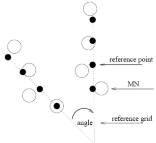
In this group based model [19-20], the nodes move around a given line, where some reference points are positioned. These reference points move together with a constant speed and every node moves randomly around its own reference point according with some entity mobility model (e.g. Random Walk). Figure 2.9 and 2.10 illustrate an example of Column movement.

Fig. 2.9 – Movement of nodes using the Column Model

Fig. 2.10 – Moving pattern of nodes using the 3-D Building Model

2.3.2. Nomadic Community

In this model [19-20] all the nodes belonging to a group move around a single reference point. Within each group, every mobile node is associated to an area where it can move in randomly. These areas cannot overlap, so the nodes maintain their own personal “spaces” (see Fig. 2.11).

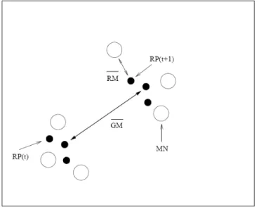
2.3.3. Pursue

In this model [19-20] the nodes pursue a particular moving target, as illustrated in Figure 2.12. The position of each node is given by:

New.pos=Old.pos+Acceleration·(Target-Old.pos)+Random.vector

Where Acceleration·(Target-Old_pos) is the movement towards the target and Random_vec is a random offset of each node obtained via an entity mobility model.

Fig. 2.11 – Movement of nodes using the Nomadic Community Model

2.3.4. Reference Point Group (RPGM)

This model [18] is a generalization of the previous three mobility models. Like in the Column, in this model the reference points move together with the same speed and direction, but, unlike the Column, they are not positioned in a line (see Fig. 2.13).

Fig. 2.11 – Movement of nodes using the RPGM

2.3.5. Contraction

In this model the nodes move towards a fixed target from all directions. For each time interval, every node calculates its new speed and pause time.

2.3.6. Expansion

This model is the opposite of the Contraction Model, and the nodes move away from the target.

2.4. SCENARIOS

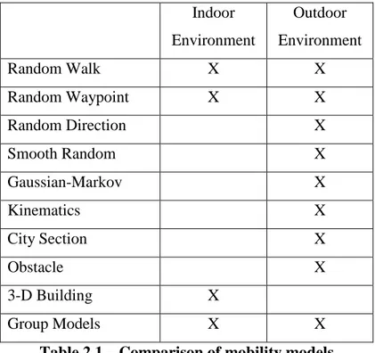
In real life the behaviour of mobile nodes depends strongly on the environment they move in. For that reason, a mobility model usually is not able to represent all the possible scenarios. For example the features of indoor movement are generally different from the outdoor ones and a synthetic model is usually designed to mimic just one of the two. Table 2.1 shows which kinds of environments the models previously described can mimic.

Indoor Environment Outdoor Environment Random Walk X X Random Waypoint X X Random Direction X Smooth Random X Gaussian-Markov X Kinematics X City Section X Obstacle X 3-D Building X Group Models X X