Disordered XY models

Scuola Normale Superiore di Pisa

Tesi di perfezionamento

D isor d er ed X Y m o d els

C on t en t s

1 Introduction 5

1.1 Disordered XY models . . . 5

2 RPXY models in two and three dimensions 9 2.1 2D RPXY models . . . 9

2.1.1 Introduction . . . 9

2.1.2 The phase diagram . . . 10

2.2 3D RPXY models . . . 14

2.2.1 Introduction . . . 14

2.2.2 The phase diagram . . . 15

2.3 Experimental realizations . . . 19

2.3.1 Josephson Junction Arrays (JJA) . . . 19

2.3.2 Cold atoms and optical lattices . . . 20

3 Quasi long range order in the 2D RPXY models 23 3.1 Random spin wave theory . . . 24

3.2 QLRO in RPXY models . . . 26

3.2.1 Monte Carlo results . . . 27

3.2.2 Quasi long range order . . . 27

3.3 Conclusions . . . 31

4 Magnetic and glassy behavior in the 2D RPXY models 33 4.1 Critical behavior at the para-QLRO transition . . . 35

4.1.1 Critical behavior approaching the pure XY transition point . . . 36

4.1.2 Critical behavior of the magnetic correlations at fixed σ 38 4.1.3 Quartic couplings . . . 41

4.1.4 Critical behavior of the overlap correlations . . . 44

4.1.5 Critical behavior along the N line . . . 46

4.2 Glassy critical behavior at T = 0 . . . 49

4.2.1 MC simulations . . . 49

4.2.2 Evidence for a T = 0 glassy transition at σ = 2/3 . . . 50

CONTENTS

4.2.4 The critical exponent ηo . . . 53

4.2.5 Results for the gauge-glass model . . . 56

4.2.6 The quartic coupling go and universality . . . 56

4.2.7 Behavior of the magnetic correlation functions . . . . 57

4.3 Conclusions . . . 60

5 Magnetic, glassy, and multicritical behavior in the 3D CR-PXY model 63 5.1 Critical behavior at the para-ferro transition . . . 65

5.1.1 Determination of Tc and ν . . . 67

5.1.2 Uo 4 and U22: universality . . . 70

5.2 Glassy behavior at finite temperature . . . 72

5.2.1 Monte Carlo simulations . . . 72

5.2.2 Tg and ν in the CRPXY model: finite size analysis . . 73

5.2.3 The exponent ηo . . . 74

5.2.4 The 3D gauge glass . . . 76

5.2.5 Numerical results . . . 76

5.2.6 The quartic couplings U₄o and U₂₂o: universality . . . . 81

5.3 Multicritical behavior on the Nishimori line . . . 83

5.3.1 Theoretical considerations about multicritical points . 84 5.3.2 Monte Carlo simulations . . . 85

5.3.3 Determination of Tc and ν . . . 86

5.3.4 The exponent η . . . 89

5.3.5 Universality . . . 92

5.3.6 Multicritical behavior . . . 94

5.4 The ferro-glassy transition . . . 95

5.4.1 Monte-Carlo results . . . 96

5.5 Conclusions . . . 98

A Monte Carlo simulation details 101 A.1 The algorithms . . . 101

A.2 Data analysis . . . 103

A.2.1 Bias correction . . . 104

B The pure XY model in two dimensions 107 B.1 The 2D XY model . . . 107

B.2 Spin wave theory in the 2D XY model . . . 110

Bibliografy 112

1

In t r o d u ct ion

1.1

D isor d er ed X Y m o d els

The study of the effects of disorder in real materials is of the utmost im-portance since no experimental sample can be considered perfect and ho-mogeneous. There are indeed many possible ways in which disorder can affect a system, for example by the presence of impurities or vacancies. In the framework of critical phenomena the main interest in disorder comes from the effects on phase transitions. The fate of the transition after the introduction of disorder can be diverse. Since the main effect is to weaken the correlations, the mildest consequence one can expect is that the critical temperature of the phase transition is lowered, but the critical behavior of the model is still governed by the pure model universality class (the disorder is irrelevant). However in general for a continuous phase transition a change of the universality class can occur. In this case the disorder is a relevant (in the renormalization group language) perturbation. In the most common scenario the critical behavior of the system is governed by a new fixed point which in the limit of vanishing disorder connects with the pure system fixed point. An even more dramatic possibility is that the transition temperature is pushed down to zero or the criticality is completely washed out. The spin systems have represented so far one of the most important theoretical mod-els where physicists probe the effects of disorder. One important example is provided by the spin glass models [1] [2] [3] [4], which may be considered as theoretical laboratories where the combined effects of quenched disorder and frustration can be studied. These models, although simplified versions, re-tain the main features of physical systems showing glassy phases. Within the realm of disordered spin systems many theoretical and numerical works have been devoted to the study of the phase diagrams and magnetic and glassy critical behaviors of Ising-like spin glasses, but much less is known about the thermodynamic properties of spin models with continuous symmetries. Among the spin glass models with continuous symmetry an interesting class

1.1. DISORDERED XY MODELS

of systems are the XY models with random phase shifts (RPXY) defined by H ≡ JX hxyi Re ¯ψxUxyψy = J X hxyi cos(θx− θy+ Axy) (1.1)

where ψx are unit vectors ψx≡ eiθx θx ∈ [0, 2π] and Uxy ≡ eiAxy. Here Axy are quenched random uncorrelated phase shifts with a certain distribution P (Axy). The RPXY models are simplified models that describe for example Josephson-junctions-arrays with positional disorder in two and three dimen-sions or the vortex-glass transition in disordered granular superconductors (more details about the experimental relevance of these models are reported in section 2.3). The aim of this thesis is to present some of our results con-cerning the effects of quenched disorder in the RPXY models in two and three dimensions. The following chapters concern several RPXY models which differ in the choice of the distribution P (Axy). In particular by the gaussian choice P (Axy) ∝ exp µ −A 2 xy 2σ ¶ (1.2) we define the GRPXY model, while the cosine distribution (appearing in the gauge theory of spin glasses [3])

P (Axy) ∝ exp µ cos Axy σ ¶ (1.3) defines the CRPXY model. It should be noted that in the limit σ → 0 the pure 2D or 3D XY model is recovered, while for σ → ∞ the so called gauge glass is obtained, where the phase shifts are uniformly distributed. This work is organized as follows:

• In Chapter 2 we define the two and three dimensional RPXY models (respectively in section 2.1 and 2.2). Then we describe their phase diagrams reviewing the available results in the literature and focusing on the aspects which have been investigated in our work. In section 2.3 we give some details about the experimental realizations of the 2D and 3D RPXY models focusing mainly on the relevance for the Josephson Junctions Arrays (in subsection 2.3.1) and on the perspectives in the field of cold atoms and optical lattices (in 2.3.2).

• In Chapter 3 we investigate the behavior of the 2D RPXY models (both the GRPXY and CRPXY) at low temperatures and for low disorder. In section 3.1 we review in particular the random spin wave theory which describes the behavior of the models in this phase. In section 3.2 we give robust numerical evidence that both models exhibit quasi-long-range-order (QLRO) and are fully described by the random spin wave theory. The general conclusions are drawn in section 3.3.

1.1. DISORDERED XY MODELS

• In Chapter 4 we investigate the 2D RPXY models (both the GRPXY and the CRPXY models) in different regions of the phase diagram. In section 4.1 we study the critical behavior along the para-QLRO transition line in both the magnetic and overlap sectors for low dis-order (small σ). Our main result is that in the magnetic sector the phase transition belongs to the usual 2D XY universality class (sec-tion 4.1.2), while the critical behavior in the overlap sector depends on the disorder (see section 4.1.4). Finally we provide compelling evi-dence of multicriticality in the overlap sector on the Nishimori line for the CRPXY model (in section 4.1.5). In section 4.2 we investigate the glassy behavior for high disorder and low temperatures. In particular by high precision Monte Carlo simulations we rule out the possibility of a finite temperature glassy transition in the 2D RPXY models and in the 2D gauge glass. Then the scenario with a T = 0 glassy transi-tion is carefully checked (sectransi-tion 4.2.2 for the RPXY and 4.2.5 for the 2D gauge glass). In particular our analysis supports a T = 0 transition in the RPXY and 2D gauge glass described by the same universality class, the 2D gauge glass universality class (see section 4.2.6). The general conclusions are drawn in section 4.3.

• Chapter 5 is devoted to the study of the CRPXY model in three di-mensions. In section 5.1 we investigate the critical behavior at the para-ferro transition line. Our main result is that the disorder is ir-relevant and the phase transition occurring on the line is described by the 3D XY universality class. In section 5.2 we investigate the high disorder low temperature region in the CRPXY model and the 3D gauge glass. We observe a finite temperature glassy transition occur-ring in both models (see section 5.2.2 and 5.2.3 for the RPXY models and 5.2.4 for the 3D gauge glass). We show that the two transitions belong to the same universality class, the 3D gauge glass universal-ity class (see section 5.2.6). In section 5.3 by high precision Monte Carlo simulations we show that on the Nishimori line the CRPXY model exhibits multicritical behavior. The topic of section 5.4 is the critical behavior on the transition line separating the glassy phase at high-disorder from the ferromagnetic phase at small σ and low T. We investigate the critical behavior and provide evidence that the transi-tion line shows reentrant behavior. Summary and general conclusions are in section 5.5.

This thesis is based on the following papers:

• Alba V Pelissetto A Vicari E 2009, Quasi-long-range order in the 2D XY model with random phase shifts J. Phys. A 42 295001

1.1. DISORDERED XY MODELS

the square-lattice XY model with random phase shifts J. Stat. Mech. P03006

• Alba V Vicari E, 2010 The three-dimensional gauge-glass model arX iv:cond-mat/1012.2432

Other papers resulting from my research in disordered and frustrated spin systems are:

• Alba V Pelissetto A Vicari E, 2008 The uniformly frustrated two-dimensional XY model in the limit of weak frustration J. Phys. A 41 175001

2

R P X Y m o d els in t wo a n d

t h r ee d im en sion s

2.1

2D R P X Y m o d els

The two-dimensional XY model with random phase shifts (RPXY) describes the thermodynamic behavior of several disordered systems, such as Joseph-son junction arrays with geometrical disorder [5–11], magnetic systems with random Dzyaloshinskii-Moriya interactions [12], crystal systems on disor-dered substrates [13], and vortex glasses in high-Tc cuprate superconduc-tors [14–18], see [4, 19] for recent reviews. The RPXY model is defined by the partition function

Z({A}) = exp(−H/T ), H = −X hxyi Re ¯ψxUxyψy = − X hxyi cos(θx− θy− Axy), (2.1) where ψx ≡ eiθx, Uxy ≡ eiAxy, and the sum runs over the bonds hxyi of a square lattice. The phases Axy are uncorrelated quenched random vari-ables with zero average. In most studies they are distributed with Gaussian probability PG(Axy) ∝ exp à −A 2 xy 2σ ! . (2.2)

We denote the RPXY model with distribution (2.2) by GRPXY. We also consider the RPXY model with distribution (cosine model)

PC(Axy) ∝ exp µ cosAxy σ ¶ , (2.3)

which we denote by CRPXY. Such a model is particularly interesting be-cause the distribution (2.3) allows some exact calculations along the so-called

2.1. 2D RPXY MODELS

Nishimori (N) line T ≡ 1/β = σ. In both GRPXY and CRPXY models the pure XY model is recovered in the limit σ → 0, while the so-called gauge glass model [16] with uniformly distributed phase shifts is obtained in the limit σ → ∞. The nature of the different phases arising when varying the temperature T and the disorder parameter σ and the critical behavior at the phase transitions have been investigated in many theoretical and exper-imental works [4–59]. In the following section we present the phase diagram of the models.

2.1.2 T h e p h a se d ia gr a m

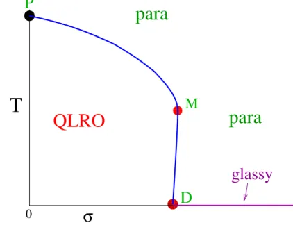
The T -σ phase diagram for the GRPXY and CRPXY models, which is sketched in Fig. 2.1, presents two finite-temperature phases: a paramag-netic phase and a low-temperature phase which shows quasi-long-range or-der (QLRO) for sufficiently small values of σ. To describe this phase the random spin wave scenario has been proposed [12]. In this scenario the long distance behavior is essentially identical to that in the model obtained by replacing

cos((θx− θy− Axy) → 1 − 1

2(θx− θy− Axy)

2 _(2.4)

in the Hamiltonian (2.1) (see [58] or Chapter 3). The paramagnetic phase is separated from the QLRO phase by a transition line, which starts from the pure XY point (denoted by P in Fig. 2.1) at (σ = 0, T = TXY ≈ 0.893) and ends at a zero-temperature disorder-induced transition denoted by D at (σD, T = 0). In the absence of disorder (σ = 0) the model shows a high-T paramagnetic phase and a low-T phase characterized by QLRO controlled by a line of Gaussian fixed points, where the spin-spin corre-lation function h ¯ψxψyi decays as 1/rη(T ) for r ≡ |x − y| → ∞, with η depending on T . The two phases are separated by a Kosterlitz-Thouless (KT) transition [60] [61] [62] [63] [64] at βXY ≡ 1/TXY = 1.1199(1). For τ ≡ T/TXY − 1 → 0+, the correlation length and the magnetic suscepti-bility diverge exponentially as lnξ ∼ τ−1/2 and χ ∼ ξ7/4 respectively. The transition along the line is believed to be of the KT-type. Indeed it has been shown [59] (see also Chapter 4 section 4.1) that in the magnetic sector the transition is described by a KT ( for example it is η = 1/4 all along the line), although in the overlap sector it depends on the disorder σ. The QLRO phase can extend up to a maximum value σM of the disorder param-eter, which is related to the point M ≡ (σM, TM), where the tangent to the transition line is parallel to the T axis 1. This important result has been 1_{We mention that the first renormalization-group (RG) analyses based on a}

Coulomb-gas description [12] predicted σD= 0, but it was later clarified that this was an artefact of

the approximations. Indeed, experimental [23] and numerical works [7, 8, 23, 35] as well as refinings of the RG arguments [20, 30, 32, 33, 36, 40], have shown the absence of a reentrant transition for sufficiently small values of σ.

2.1. 2D RPXY MODELS

proven for the CRPXY model [20], moreover the critical value σD at T = 0 has to satisfy σD ≤ σM. No long-range glassy order can exist at finite tem-perature, in fact it has been proven [28,29] that the lower critical dimension for the glassy ordering is above two for these systems. Although this does not exclude in principle more exotic low-temperature glassy phases [45, 52], for example a phase characterized by glassy QLRO, it turns out that the model undergoes a T = 0 glassy transition [59] (see also Chapter 4) and no glassy phase is present at finite temperature. In the limit σ → ∞ the phases are uniformly distributed and the XY gauge glass model is obtained. This model has been much investigated [10,14–18,24–29,31,34,37–39,41,43,45,46,48–57]. Several numerical studies [27,41,48,50,51,54–56] support a zero-temperature glassy transition, as in the 2D RPXY models. According to this scenario, the correlation length determined from the overlap correlation function di-verges as ξo ∼ T−ν when approaching the critical point T = 0. The critical exponent ν has been estimated by finite-temperature Monte Carlo (MC) simulations, obtaining [50] 1/ν = 0.39(3) and [54] 1/ν = 0.36(3). The exponent ν is related to the T = 0 stiffness exponent θ by θ = −1/ν. The T = 0 numerical calculations of [48] and [56] provided the estimates θ = −0.36(1) and θ ≈ −0.45 respectively, which are consistent with the finite-temperature estimates of ν. The T = 0 transition scenario had been questioned in [10,11,45,46,49,52,53,57], which provided some numerical and experimental (for Josephson-junction arrays with positional disorder [11]) evidence for the existence of a finite-temperature transition at T ≈ 0.2, with a low-temperature glassy phase characterized by frozen vortices and glassy QLRO. However, recent large scale Monte Carlo simulations provide con-clusive evidence supporting the T = 0 glassy transition [59]. More precisely the upper bound Tc < 0.01 was obtained and the estimate 1/ν = 0.40(2), in agreement with earlier works. Besides, it was also proven that the T = 0 glassy transition occurring in the RPXY models and in the 2D gauge glass belong to the same universality class (see Chapter 4 and in particular sec-tion 4.2 for the details). Other features of the phase diagram of the RPXY models are better discussed within the CRPXY model, characterized by the random phase-shift distribution (2.3), because of the existence of exact results along the so-called Nishimori (N) line [20, 22]

T ≡ 1/β = σ. (2.5)

Along the N line the energy density E is known exactly: E ≡ 1

V[hHi] = −2 I1(β) I0(β)

, (2.6)

where I0(β) and I1(β) are modified Bessel functions. Moreover, the spin-spin and overlap correlation functions are equal:

2.1. 2D RPXY MODELS 000 000 000 000 111 111 111 111 00 00 00 11 11 11 0

T

QLRO

σ

D

P

M

para

para

glassy

Figure 2.1: Phase diagram of RPXY models as a function of T and of the disorder-distribution variance σ.

As already noted in [22], the N line plays an important role in the phase diagram, because it marks the crossover between the magnetic-dominated region and the disorder-dominated one. This fact suggests in particular that the point M in the phase diagram could be a multicritical point, as confirmed by the analysis in [59] (see also Chapter 4 and section 4.1.5). It is worth noting how similar the phase diagrams of the CRPXY model and of the square-lattice ±J Ising model in the T -p plane are, see Figs. 2.1 and 2.2, respectively. The square lattice ±J (Edwards-Anderson) Ising model is defined by the Hamiltonian

H±J = − X hxyi

Jxyσxσy, (2.8)

where σx = ±1, the sum is over pairs of nearest-neighbor sites of a square lattice, and Jxy are uncorrelated quenched random variables, taking values ±J with probability distribution P (Jxy) = pδ(Jxy− J) + (1 − p)δ(Jxy+ J). This model presents an analogous N line [65] in the T -p phase diagram, defined by tanh(1/T ) − 2p + 1 = 0. The transition point along the N line is a multicritical point (M) [66, 67]. Moreover, the critical behavior for T > TM N P and T < TM N P is different. From the pure Ising point at p = 1 to the MNP the critical behavior is analogous to that observed in 2D randomly dilute Ising (RDI) models [68]. From the MNP to the T = 0 axis the critical behavior belongs to a new strong-disorder Ising (SDI)

2.1. 2D RPXY MODELS 00 00 00 00 00 11 11 11 11 11 00 00 00 00 11 11 11 11

0

T

ferro

MNP

Is

glassy

Is

= +log

RDI

1 − p

para

SDI

N line

Figure 2.2: _{Phase diagram of the ± (Edward-Anderson) Ising model on the square} lattice. The phase diagram is symmetric under p → 1 − p.

universality class [69]. Finally, the T = 0 end-point of the low-temperature paramagnetic-ferromagnetic transition line is the starting point of a T = 0 transition line, characterized by a glassy universal critical behavior [70]. In [20] it was also argued that in the RPXY models (in particular, in the CRPXY one) the low-temperature paramagnetic-QLRO transition line from the critical point M to the point D runs parallel to the T axis, so that σD = σM. The same arguments fail in the 2D ±J Ising model [66, 67, 69, 71, 72], although they provide a good approximation. Thus, they are likely not exact also in the case of the RPXY models, suggesting that 0 < σM − σD ≪ σM. In the phase diagram reported in Fig. 2.1, which refers to the CRPXY, we may distinguish two transition lines meeting at point M : the thermal paramagnetic-QLRO transition line from P to M , which can be approached by decreasing the temperature at fixed σ, and the transition line from M to D, which can be instead observed by changing disorder at fixed T for sufficiently low temperatures. The phase transition from the paramagnetic to the QLRO phase is generally expected to be of KT type (ln ξ is expected to have a power-law divergence). Some numerical results supporting the KT-like behavior were presented in [35]. We mention that [59] (see also Chapter 4 section 4.2.7) provides further evidence supporting this scenario. The disorder-driven T = 0 transition at σD has been argued [21, 30, 35, 40, 47] to show a KT-like behavior with ln ξ ∼ (σ − σD)−1 and χ ∼ ξ2−η with

2.2. 3D RPXY MODELS

η = 1/16. However, other RG studies [33, 36] obtained a different behavior: ln ξ ∼ (σ − σD)−1/2. The value of η associated with the magnetic two-point function is believed to vary along the critical line [12,30,33,36], from η = 1/4 of the pure XY model at σ = 0 to η = 1/16 at the T = 0 transition.

2.2

3D R P X Y m o d els

The 3D XY model with random phase shifts RPXY is defined by the same interaction defining the 2D RPXY models

Z({A}) = exp(−H/T ), H = −X hxyi Re ¯ψxUxyψy = − X hxyi cos(θx− θy− Axy), (2.9)

where ψx ≡ eiθx, Uxy ≡ eiAxy, and the sum runs over the bonds hxyi of a cubic lattice. The phases Axy are uncorrelated quenched random vari-ables with zero average. The model describes XY-magnets with random Dzyaloshinskii-Moriya interactions [12], 3D Josephson-junctions arrays with positional disorder [5, 6] and vortex glasses [14–16]. Concerning P (Axy) the same definitions used for the 2D case hold. In particular the gaussian dis-tribution PG(Axy) ∝ exp à −A 2 xy 2σ ! . (2.10)

defines the GRPXY model and the Nishimori distribution PC(Axy) ∝ exp µ cosAxy σ ¶ , (2.11)

the CRPXY model (cosine model). In this thesis we will treat only the CRPXY model, although the features of the two models are expected to be qualitatively the same. As for the 2D model this distribution allows some exact results on a particular line on the phase diagram, the so called Nishimori line T ≡ 1/β = σ [20, 22]. In particular the energy density E is known exactly:

E ≡ _V1[hHi] = −2I_I1(β) 0(β)

, (2.12)

where I0(β) and I1(β) are modified Bessel functions. Furthermore it is worth to remind that on the Nishimori line the spin-spin and overlap correlation functions are equal:

[h ¯ψxψyi] = [|h ¯ψxψyi|2]. (2.13) The pure 3DXY model is recovered in the limit σ → 0, while the so called 3D gauge glass [16] model is obtained in the limit σ → ∞.

2.2. 3D RPXY MODELS

2.2.2 T h e p h a se d ia gr a m

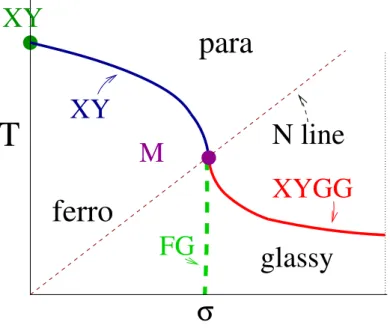
In this section we review the phase diagram of the 3D RPXY model in the T − σ plane (see Fig. 2.3). In absence of disorder (σ = 0) the model shows a high-T paramagnetic phase and a low-T ferromagnetic ordered phase char-acterized by the standard 3D XY behavior. The transition between the two phases is marked by the 3DXY critical point βc ≡ 1/Tc = 0.45420(2). At this point the system exhibits the 3DXY critical behavior characterized by the critical exponents ν = 0.67155(27) η = 0.0380(4) α = 0.0146(8) γ = 1.3177(5) (see for example [73] and reference therein). For low values of the disorder σ there are arguments suggesting that for the GRPXY model the ferromagnetic ordered phase survives [74]. It is plausible that this re-sult holds also for the CRPXY. The ferromagnetic phase is separated from the paramagnetic high temperature phase by a transition line (XY-M in Fig. 2.3) which starts at the 3D XY point and ends at the Nishimori point M (at TM = σM = 0.7840(2) [76]). For non zero values of σ the phase tran-sition on the line XY-M has not been investigated so much. One possible scenario is that the disorder is an irrelevant parameter and the universal-ity class of the transition is the 3DXY universaluniversal-ity class. One argument in favor of this scenario is provided by the Harris criterion [75] which states that for dν < 2, where ν is the exponent of the pure model, the disorder is irrelevant. For the 3DXY model it is 2 − dν ≈ −0.01 suggesting that even though the disorder is irrelevant it would be hard to check it in finite size systems. Actually, this scenario has been confirmed in [76] (see also Chapter 5 and section 5.1), where it has been proven that the transition is of the 3D XY type on the line and the only effect of the disorder is to introduce very slow scaling corrections. In the limit σ → ∞ the phase shifts Axy are uniformly distributed and the 3D gauge glass model is obtained. This model has been intensively investigated and there is now consensus on a finite temperature glassy transition. According to the accepted scenario the system undergoes a glassy transition at Tc= 0.460(15) [77] and the cor-relation length ξo determined from the overlap correlation function diverges as ξo ≈ T−ν approaching Tc. The obtained value for ν from numerical sim-ulations is ν = 1.39(5) [77]. A quite larger value ν = 3.2(4) was obtained in [76], where significantly larger lattice sizes than in earlier works were simulated. Analogously the overlap susceptibility diverges as χo ≈ L2−ηo. The exponent ηo has been also determined, we quote the most recent re-sults [77] ηo = −0.47(7) and [76] ηo = −0.47(2). In [76] it was shown that the transition at σ → ∞ is not isolated, but the 3D RPXY models exhibit glassy transitions at finite temperature for every σ > σM (see also Chapter 5 and sections 5.2.2 5.2.3). Moreover all these transitions belong to the 3D gauge glass universality class. Therefore a critical line starting at M divides the glassy phase at low temperatures from the paramagnetic phase (the red line in Fig. 2.3). At low temperatures the glassy phase is separated from the

2.2. 3D RPXY MODELS

T

para

M

glassy

ferro

XY

N line

XY

XYGG

FG

σ

Figure 2.3: Phase diagram of the CRPXY model as a as function of the temper-ature T and of the disorder variance σ.

ferromagnetic ordered phase by a transition line starting from the Nishimori point M ≡ (TM, σM) and ending at T = 0. The critical properties of the model on this transition line have not been investigated much. An impor-tant result has been obtained by Nishimori: the value σ = σM is un upper bound for the maximum value where the ferromagnetic order can exist. At the point (σM, TM) the transition line runs parallel to the temperature axis. It was argued that the transition line remains parallel to the T axis up to T = 0. However, as we already mentioned in the previous sections, a similar argument fails for the 3D ± J Ising model where the transition line shows a slightly reentrant behavior [66, 67, 69, 71, 72]. This hypothesis is weakly confirmed by the numerical analysis in [76]. The Nishimori line (and the Nishimori point M) plays an important role in the phase diagram, since it divides the magnetic-dominated region from the overlap-dominated one. For the 3D ± J Ising model it has been shown that the Nishimori point M is a multicritical point (see [78]). We also recall that multicriticality around M has been observed in the 2D case (see the previous section about the 2D RPXY models). The same type of scenario has been settled recently for the 3D CRPXY model in [76] (see also section 5.3 for the details), where the estimates of the RG exponents y1 = 1/ν = 0.93(3) y2 = 0.57(3) of the two relevant operators at the multicritical point have been obtained. We remark that, as already observed for the 2D RPXY models, there are many

2.2. 3D RPXY MODELS

similarities between the phase diagram of the 3D RPXY models and that of the 3D Edward-Anderson Ising model [79]. This model is defined by the interaction

H = −X hxyi

Jxyσxσy (2.14)

where σx = ± are Ising variable and Jxy are uncorrelated quenched random variables taking the values ±J with probability P (Jxy) = pδ(Jxy− J) + (1 − p)δ(Jxy+J). The phase diagram (see Fig. 2.4) is quite rich and has been in-vestigated in many works [73] [78] [80] [81] [82] [83] [84] [85] [86] [87] [88] [89]. For p = 1 the standard 3D Ising model is recovered. The high-temperature

2.2. 3D RPXY MODELS

Ising (RDIs) universality class, [78, 83] characterized by the magnetic criti-cal exponents [73, 78] νf = 0.683(2) and ηf = 0.036(1). The Ising transition at p = 1 is a multicritical point and, close to it, for 0 < 1 − p ≪ 1, one observes multicritical behavior [78, 84, 85]. The paramagnetic-glassy (PG) transition line starts from the MGP and extends up to p = 1/2. The exper-imental realizations of the ± J Ising model are scarce although it describes well the glassy behavior of materials with strong magnetic anisotropy like Fe1−xMnxTiO3 and Eu1−xBaxMnO3, (see [80] [81] [82]). The main reason is that most of the experimental materials are made of Heisenberg like spins with O(3) symmetry and weak magnetic anisotropy. For this types of sys-tems it turns out that the experimental estimates of the critical exponents associated to the glassy behavior are incompatible with the Ising universality class. We mention that all the experiments for typical magnetic systems give νg ≈ 1.3 − 1.4 ηg ≈ 0.4 − 0.5 (see [90] [91] [92] [93] [94] [95] [96]). For these type of systems, models with continuous degrees of freedom, such as the 3D RPXY model, are in general expected to provide a better approximation. Another well studied model with continuous symmetry is the Heisenberg model defined by

H = −X hxyi

JxyS~xS~y (2.15)

where ~Sx are three dimensional unit vectors. From the symmetry point of view this model, having the full O(3), is the natural candidate to describe glassy order in real materials, particularly for those materials with weak magnetic anisotropy. Despite the many efforts over the last 30 years [97–118] the phase diagram of this model has not been clarified. A lot of efforts have been put to understand whether a glassy transition occurs at finite temperature or not, although no compelling evidence has been found so far. In fact early numerical simulations (see for example [97]) suggested that the model has only a zero temperature glassy transition in contrast with experiments. After that a new scenario (see [103]) has been put forward, the so called spin-chirality decoupling. The chirality is a multispin variable defined by the product of three neighboring spins

χ ≡ ~Si· ~Sj∧ ~Sk (2.16) In this scenario at low temperatures two different transitions occur, one at lower temperature involving the spin variables and the other at higher temperature in the chiral sector of the model where only the chiral discrete symmetry Z2 is broken while the SO(3) is preserved. The claim is that the chiral transition corresponds to the transition observed in the experiments, the chirality being the correct quantity to describe the glassy behavior.

2.3. EXPERIMENTAL REALIZATIONS

2.3

E x p er im en t a l r ea liza t ion s

As we mentioned already both the 2D and 3D RPXY models have many realizations in physical systems. For example they describe the thermo-dynamic behavior of several disordered systems, such as Josephson junc-tion arrays with geometrical disorder [5–11], magnetic systems with random Dzyaloshinskii-Moriya interactions [12], crystal systems on disordered sub-strates [13], and vortex glasses in high-Tc cuprate superconductors [14–18]. Moreover in recent years the possibility to use optical lattices has widened very much the number of models that can be simulated in experiments. This is true also for the XY model in two and three dimensions. In the next two sections I will give some more details on the realizations of the RPXY model in the Josephson Junction Arrays and on possibilities with the optical lattices.

2.3.1 J osep h son J u n ct ion A r r ay s ( J J A )

The first artificially fabricated JJA were realized almost thirty years ago with the aim to develop new electronics based on superconducting devices [119]. Each Josephson junction is made of two grains of superconducting material separated by an insulating barrier. In the JJA many of these junctions are disposed on a regular bidimensional or three dimensional structure to form a lattice (see Fig. 2.5). Each junction shows the famous Josephson effect

Figure 2.5: Josephson Junction Array chip developed at NIST as a standard volt. The chip contains 3020 Josephson Junctions.

described by the two equations

I = Icsin ∆φ (2.17)

~d

dt∆φ = 2e∆V (2.18)

where I is the current and ∆V the external potential imposed on the junc-tion, while ∆φ is the phase shift between the Ginzburg-Landau order pa-rameter describing each superconducting island and Ic (Josephson critical

2.3. EXPERIMENTAL REALIZATIONS

current) is the maximum current that the junction can sustain. The first equation (DC Josephson effect) implies that even without an external im-posed potential a current flows across the junction. If an external driving potential ∆V is imposed (AC Josephson effect), then the behavior of the system is described by the second equation and an AC current with fre-quency 2e~ is observed. For temperatures well below the critical temperature associated to the transition for the single grain the relevant parameter is the phase of the wave function describing the superconductor. In this situation the JJA are a realization of the pure XY model defined by the interaction

H = −X hxyi Re ¯ψxUxyψy = − X hxyi cos(θx− θy),

ψx ≡ eiθx, θx being the phase of the wave function of the grain at position x. For temperatures above the Kosterlitz-Thouless transition, although each grain is superconducting, the system does not exhibit any superconducting phase, which is instead observed below the transition. The JJA in pres-ence of an external orthogonal uniform magnetic field are described by the uniformly frustrated XY model

H = −X hxyi Re ¯ψxUxyψy = − X hxyi cos(θx− θy− Axy),

where Axy has to be interpreted as the vector potential giving the exter-nal magnetic field. If the vector potential is non uniform we have the XY model with a nonuniform orthogonal magnetic field. This model describes Josephson junction arrays with positional disorder in presence of an ex-ternal magnetic field [7] [8]. In these systems the shape of the plaquettes forming the array structure is not uniform implying a nonuniform random flux piercing each plaquette.

2.3.2 C old a t om s a n d op t ica l la t t ices

In recent years the possibility to use optical lattices (see [120] for a nice review) has represented a real breakthrough in condensed matter physics. An optical lattice is created by using counter-propagating laser beams which give a periodic potential that may trap atoms. The atoms are then cooled and confined around the minima of the potential. This allows a lot of possi-bilities as regards for example the geometric configuration of the system, for example low dimensional lattice models can be simulated efficiently. One of the most important reasons for the success of the optical lattices is the possibility to simulate pure models, without worrying about impurities or interactions with phonons. Some laser configuration to generate one dimen-sional cigar-shaped clouds and three dimendimen-sional lattices are shown in Fig. 2.6. The most critical point is the measurement process, in fact in most of the

2.3. EXPERIMENTAL REALIZATIONS

Figure 2.6: Outline of the experimental setup (on the left) to generate different clouds of atoms configurations (on the right). The red arrows represent the laser beams.

cases it involves the destruction of the lattice. However, very recently new techniques allowing in situ measurements have been developed [121]. From the XY models perspective optical lattices give for example the opportunity to simulate directly the Josephson Junction Arrays using Bose-Einstein con-densate. This has been done for example in [122] where a one dimensional array of Josephson Junctions was considered. Furthermore one impressive achievements in the fields of quantum fluids has been the observation of the Kosterlitz-Thouless phase transition in two dimensional Bose gases [123]. In fact in two dimensional Bose fluids, due to the Mermin-Wagner theo-rem [124], thermal fluctuations prevent the onset of the Bose-Einstein con-densation. However, although true long range order order is not possible, quasi long range order can be present. Quasi-long-range order means that the two point correlation function decays algebraically

hΨ†(~r)Ψ(0)i ∝ r−η (2.19)

where we indicated with Ψ(~r) the particle creation operator at position ~r and η is a critical exponent. The authors of [123] considered a three di-mensional Bose fluid constrained in a planar geometry by a strong external potential (the experimental setup is outlined in Fig. 2.7) More precisely they considered a stack of two Bose gases of degenerate Rubidium atoms, each confined in a nearly two dimensional geometry. By suddenly switching off the confining potential and recording the matter wave interference pat-tern between the two clouds the authors were able to access the two point

2.3. EXPERIMENTAL REALIZATIONS

Figure 2.7: Experimental setup used in [123] to observe the BKT transition in Bose gases. Two laser beams were used to obtain a stack of Bose gas confined in a nearly two dimensional geometry. The measurement process is outlined in the bottom left corner. Basically it consists in switching off the confining potential and observing the matter wave interference pattern produced. On the right side the result in the quasi long-range-order regime (top) and in the high temperature phase (bottom) is reported. The dislocations observed in the high temperature regime are the signature of the free vortex proliferation in the system.

correlation function and to extract the exponent η at the transition. The result was in agreement within the error bars with the expected value in a BKT scenario (η = 1/4). To go beyond the pure XY model we men-tion that using the optical lattice set up it is possible to simulate easily the uniformly frustrated XY model. In fact a uniform vector potential can be simulated by putting the system in a rotating reference frame with constant angular velocity (see for example [125] for a recent proposal on how to simu-late uniformly frustrated Josephson Junction Arrays and [126] for a detailed discussion of rotating bosons). To simulate the RPXY models, the major challenge in the optical lattice framework is the implementation of the site dependent gauge potential Axy. However recently many different proposals have been put forward to simulate not only site dependent abelian gauge potentials (which is the case for RPXY models) but also non abelian ones (see [127] and reference therein). Therefore it is likely that this difficulty will be overcome in the future.

3

Q u a si lon g r a n ge or d er in t h e

2D R P X Y m o d els

A b st r a ct

We study the square-lattice XY model in the presence of random phase shifts. We consider two different disorder distributions with zero average shift (giving the GRPXY and CRPXY model) and investigate the low-temperature quasi-long-range order phase which occurs for sufficiently low disorder. By means of Monte Carlo simulations we determine several univer-sal quantities, namely the exponent η(T ) and the univeruniver-sal ratio ξ/L. We then compare with the analytic predictions of the random spin-wave theory. We observe a very good agreement which indicates that the universal long-distance behavior in the whole low-disorder low-temperature phase is fully described by the random spin-wave theory.

N ot a t ion s

In terms of complex site variables ψi ≡ eiθi, the RPXY Hamiltonian takes the form

H = −X hiji

Re ψ∗_iUijψj (3.1)

where Uij ≡ eiAij. We consider several two-point correlations functions: the magnetic spin-spin correlation function

Gs(x − y) ≡ Re [hψx∗ψyi] = [hψx∗ψyi], (3.2) and the overlap correlation function

3.1. RANDOM SPIN WAVE THEORY

which can be written as Go(x − y) = [h¯qxqyi], where qx = ψ(1)∗x ψx(2) and the upper scripts refer to two independent replicas with the same disorder. The angular and square brackets indicate the thermal average and the quenched average over disorder, respectively. We also consider a gauge-invariant spin-spin correlation function

Gg(x − y) ≡ [Rehψ∗xU [Γx;y] ψyi], (3.4) where Γx;y is a path that connects sites x and y and U [Γx;y] is a product of phases associated with the links that belong to Γx;y. The paths connecting the points x and y are chosen along the lattice axes ( we mention that this quantity has been already used to study the XY model in the limit of weak uniform frustration, see [128] for details). We define the corresponding susceptibilities: the magnetic susceptibility χs ≡ PxGs(x), the overlap susceptibility χo ≡ PxGo(x), and χg ≡ PxGg(x). We also define the corresponding second-moment correlation lengths

ξ_#2 _≡ Ge#(0) − eG#(qmin) ˆ

q2

minGe#(qmin)

, (3.5)

where qmin ≡ (2π/L, 0), ˆq ≡ 2 sin q/2, and eG#(q) is the Fourier transform of G#(x), and # indicates s, o, g.

3.1

R a n d om sp in wave t h eor y

The low-temperature phase of RPXY models shows QLRO for sufficiently small values of σ. The universal features of the long-distance behavior are explained by the random spin-wave theory [12], obtained by replacing

cos(θx− θy− Axy) −→ 1 − 1

3.1. RANDOM SPIN WAVE THEORY

For the CRPXY one should take into account the nontrivial dependence of P (Aij) on Aij. For the overlap correlation function one still obtains (3.9), in fact for any probability distribution Go(x − y) does not depend on randomness in the spin-wave approximation. For the spin correlation function the σ dependence at T = 0 is more complex. For σ → 0 we obtain Gs(x − y) = exp[(T + σ + σ2/2)G(x − y)], (3.11) disregarding terms of order σ3_{. The derivation of (3.11) is easy} follow-ing [12]. We first consider the spin-spin correlation function Gs(r, Aα) = hexp [i(φ(0) − φ(r))]i for fixed values of the random phases Aα. As in [12] we rewrite it as Gs(r) = hexp £ i(φ(0) − φ(r)) − βRd2_{rA · ∇φ}¤_i0 hexp£−βR d2_{rA · ∇φ}¤_i 0 , (3.12)

where h·i0 indicates the average with Hamiltonian H = β₂

Z

d2_r(∇φ)2 . (3.13)

Repeating the steps discussed in [12] we end up with Gs(r, A) = exp à T G(r) +1 2 Z d2sX α Aα(s)Mα(s, r) ! , (3.14)

where G(r) is the Gaussian propagator (3.10) and Mα(s, r) = 2 Z d2q (2π)2e −iq·s_(eiq·r − 1)q_qα₂ . (3.15) Note that Mα(s, r) is imaginary, Mα(s, r)∗ = −Mα(s, r), so that

|Gs(r, A)|2 = e2T G(r) . (3.16) Thus, as stated above, irrespective of the phase distribution, the overlap correlation function does not depend on σ. To compute the spin correlation function we must average Gs(r, A) over the distribution of the phases Aα. We consider the general distribution

P (A) ∝ exp µ −Q(A 2₎ 2σ ¶ , (3.17)

which satisfies Q(z) = z for z → 0 and is such that, for σ → 0 the distribu-tion is peaked around A = 0. Thus, to compute the expansion of Gs(r) for small σ, we can expand Q(A2) in powers of A2. We assume

3.2. QLRO IN RPXY MODELS

where α is a distribution-dependent coefficient. To compute the correction of order σ2 _{to η}

s we rewrite ([·]A indicates the average over A) S ≡ " exp à 1 2 Z d2sX α Aα(s)Mα(s, r) !# A ∝ Z [DA] exp à −_2σ1 Z d2s[A2+ α(A2)2] + 1 2 Z d2sX α AαMα ! . (3.19) We introduce a new field Bα defined by

Aα=√σBα+ σ

2Mα (3.20)

and perform the integral over B. Disregarding terms of order σ3 we obtain S = exp · σ 8 (1 − 6ασ) Z d2s M (s, r)2 ¸ . (3.21) Since

3.2. QLRO IN RPXY MODELS

3.2.1 M on t e C a r lo r esu lt s

We performed MC simulations of the GRPXY and CRPXY models, con-sidering square lattices of linear size L with periodic boundary conditions. We set in both cases σ = 0.1521, which is well below the maximum value σM (σM &0.30 in the CPRXY model [58] and σM ≃ π/8 in the GRPXY model) and considered several values of T below the critical temperature Tc(σ), which marks the end of the QLRO phase. MC simulations in the high-temperature phase [58] indicate Tc = 0.771(2) for the GRPXY and Tc = 0.763(1) for the CRPXY. In the simulations we used a mixture of stan-dard Metropolis and overrelaxed microcanonical updates: a single MC step consisted of five microcanonical sweeps followed by one Metropolis sweep. The overlap correlation functions and corresponding χo and ξo were ob-tained by simulating two independent replicas for each disorder sample. In the case of the GRPXY model we performed standard MC simulations at T = 2/3, 1/2, 2/5, for lattice sizes 10 . L . 40. Typically, we considered 50000 disorder realizations and performed O(105_{) MC steps for each of them.} In the case of the CRPXY model the parallel-tempering method [129, 130] allowed us to investigate the temperature range T < Tc down to T ≈ 0.139, which is below the N line, i.e. satisfies T < σ = 0.1521. We performed simulations for lattice sizes 10 . L . 30. Typically, we considered 25000 disorder realizations. For β ≡ 1/T = 7.2 we also performed standard MC runs up to L = 85.

3.2.2 Q u a si lon g r a n ge or d er

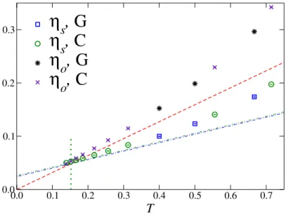
We estimate the exponents ηs and ηo by studying the finite-size behavior of the susceptibilities χs and χo. Indeed, for L → ∞ according to finite size theory they behave as

χs,o∼ L2−ηs,o . (3.27)

Estimates of χs are shown in Fig. 3.1. On a logarithmic scale, the data fall on a straight line, indicating that the asymptotic behavior (3.27) already holds for the values of L we consider. In Fig. 3.2 we show the estimates of ηs and ηo for the GRPXY and CRPXY model. For T . 0.2 they agree with the spin-wave approximations (3.24) and (3.25). Moreover, they appear to be mostly independent of the model, in agreement with the random spin-wave predictions (note that σ2_{/2 = 0.0116 for σ = 0.1521). For a more} quantitative check, in Fig. 3.3 we plot the difference 2ηs − ηo vs T , and compare it with the low-order approximations

2ηs− ηo= σ_π (GRPXY), (3.28)

2ηs− ηo= σ+σ 2_/2

π (CRPXY). (3.29)

The agreement is very good. Moreover, the above-reported relations appear to hold up to temperatures close to the KT transition Tc (for σ = 0.1521 we

3.2. QLRO IN RPXY MODELS 2 3 4 lnL -0.8 -0.4 0.0 ln χ s /L 2

β=1.4

β=7.2

Figure 3.1: MC estimates of ln χs/L2 versus ln L for the CRPXY model at σ =

0.1521 and two values of β ≡ 1/T , corresponding to T ≈ 0.139 and T ≈ 0.714.

0.0 0.1 0.2 0.3 0.4 0.5 0.6 0.7

T

η

,

G

η

,

C

η

,

G

η

,

C

Figure 3.2: The MC estimates of ηs and ηo vs T for the GRPXY and CRPXY

models at σ = 0.1521. The lines shows the spin-wave approximations (3.24), and (3.25). The two lines that give ηs for the GRPXY and CRPXY models cannot be

easily distinguished on the scale of the plot. The dotted vertical line corresponds to T = σ = 0.1521; in the CRPXY model this point belongs to the N line.

have Tc = 0.771(2) for the GRPXY model and Tc= 0.763(1) for the CRPXY model), suggesting that they may also hold at the KT transition. Since MC

3.2. QLRO IN RPXY MODELS 0.0 0.2 0.4 0.6 0.8

T

2η

−η

Figure 3.3: We plot the difference 2ηs− ηo vs T at σ = 0.1521, and compare it

with the low-order spin-wave approximations for the GRPXY and CRPXY models, cf. (4.23) and (4.24), respectively dotted and dashed lines. The vertical dotted and dashed lines indicate the critical temperatures of the two models, i.e. Tc= 0.771(2)

and Tc= 0.763(1) for the GRPXY and CRPXY, respectively.

simulations in the high-temperature phase [58] show a clear evidence that ηs= 1/4, this may suggest that at the KT transition

ηo≈ 1 2− σ π (GRPXY), (3.30) ηo≈ 1 2 − σ + σ2/2 π (CRPXY), (3.31)

The most important check of the spin-wave nature of the QLRO is provided by the MC data shown in Figs. 3.4, where we plot Rs vs ηs and Ro vs ηo: they agree with high accuracy with the curves Rs(ηs) and Ro(ηo) computed in the spin-wave limit. We believe that these results provide a conclusive evidence that the QLRO phase is determined by random spin-wave theory. Finally, we report some results for the gauge-invariant correlation function (3.4), see Fig. 3.5. In the spin-wave limit one finds [22]

[hei(φx−Ax,x′−...Ay′,y−φy)

i] = exp[(T − σ)G(x − y) − |x − y|σ/2], (3.32) which predicts that gauge-invariant spin-spin correlation functions are not critical. For instance, in the large-L limit the correlation length ξg(gap)defined from the large-distance exponential decay of the gauge-invariant correlation function is finite and given by ξg(gap) = 2/σ, independently of T . These

3.2. QLRO IN RPXY MODELS 0.00 0.05 0.10 0.15 0.20 0.25

η

R

η

R

Figure 3.4: Rs ≡ ξs/L versus ηs (above) and Ro ≡ ξo/L versus ηo (below).

The full lines are the results of the random spin-wave theory, obtained by using the expressions (3.26). The MC data are obtained for the CRPXY and GRPXY models with σ = 0.1521.

3.3. CONCLUSIONS 0 10 20 30 40

L

T=2/3,

ξ

T=1/2,

ξ

T=2/5,

ξ

T=2/3,

ξ

T=1/2,

ξ

T=2/5,

ξ

Figure 3.5: The correlation lengths ξs, defined from the standard spin-spin

corre-lation function, and ξgdefined from a gauge invariant spin-spin correlation function,

versus L. Results for the GRPXY model with σ = 0.1521.

predictions are confirmed by our MC simulations. We compute the second-moment correlation function ξg defined in (3.5). The results are reported in Fig. 3.5. It is evident that ξg is finite in the large-L limit, satisfies ξg . 2/σ ≃ 13, and is independent of T . Again, this result shows that the critical behavior is correctly described by the spin-wave theory.

3.3

C on clu sion s

We have studied the low-temperature low-disorder phase in RPXY models. We have considered two different disorder distributions and for each of them we have computed numerically the exponents ηs and ηo, and the correlation lengths ξs and ξo. These results have been compared with the predictions of the random spin-wave theory. The ratios ξs/L and ξo/L, when expressed in terms of the corresponding exponents ηs and ηo, are in perfect agreement with the analytic predictions. This indicates that the expressions (3.26) hold quite precisely in the whole low-temperature QLRO phase. Moreover, the difference 2ηs− ηo is apparently well described by spin-wave theory up to the critical transition which marks the end of the paramagnetic phase. In agreement with the random spin-wave theory, the gauge-invariant spin correlation function (3.4) is not critical. Finally, note that our calculations refer to probability distributions for which [A] = 0. Very little changes if we

3.3. CONCLUSIONS

consider a nonzero average; for instance, one might use the distribution P (A) ∝ exp£−(A − a)2/2σ¤ . (3.33) In this case we have [A] = a. The new model can be mapped into the original one by performing the gauge transformation

ψ_(x′ _1,x2)= e−ia(x1+x2)_ψ

x1,x2 A ′

ij = Aij − a. (3.34) Hence this model has the same phase diagram as the original one. The transformation (3.34) leaves the overlap correlation functions unchanged, since they are gauge invariant. The behavior of the spin-spin magnetic correlation functions is more subtle. If b = (a, a), in Fourier space we have

e

Gs(q; a) = eGs(q + b; a = 0), (3.35) where eGs(q; a) is the Fourier transform of the spin magnetic correlation function in the theory with a non-vanishing average a. In the standard theory (a = 0) the critical modes are those with q = 0, while for q 6= 0 the behavior is not critical. This implies that the critical modes in the theory with a 6= 0 are those associated with a non-vanishing momentum q = −b. Hence, in this theory the magnetic susceptibility, which corresponds to q = 0, is not critical.

4

M a gn et ic a n d gla ssy

b eh av ior in t h e 2D R P X Y

m o d els

A b st r a ct

We investigate the magnetic and glassy transitions of the square-lattice XY model in the presence of random phase shifts. We consider both the GRPXY and the CRPXY models. We perform Monte Carlo simulations for several values of the temperature and of the variance of the disorder distribution, in the paramagnetic phase close to the magnetic and glassy transition lines (see Fig. 4.1). We find that, along the transition line separating the paramag-netic and the quasi-long-range order phases, magparamag-netic correlation functions show a universal Kosterlitz-Thouless behavior as in the pure XY model, while overlap correlations show a disorder-dependent critical behavior. This behavior is observed up to a multicritical point which, in the CRPXY model, lies on the Nishimori line. Finally, for large values of the disorder variance, we observe a universal zero-temperature glassy critical transition, which is in the same universality class as that occurring in the gauge-glass model.

N ot a t ion s

We consider RPXY models defined on square lattices of size L2with periodic boundary conditions. We define the magnetic spin-spin correlation function G(x − y) ≡ [h ¯ψxψyi] (4.1) and the overlap correlation function

0.0 0.1 0.2 0.3 0.4 0.5 0.6

σ

T

Figure 4.1: _{Values of T ≡ 1/β and σ where MC data were collected. The circles} and crosses refer to the GRPXY and CRPXY models, respectively. The dotted line T = σ

4.1. CRITICAL BEHAVIOR AT THE PARA-QLRO TRANSITION 00 00 00 00 11 11 11 11 000 000 000 111 111 111 0

T

QLRO

σ

D

P

M

para

para

glassy

Figure 4.2: Phase diagram of RPXY models as a function of T and of the disorder-distribution variance σ.

where µ ≡ Pxψx and V = L2. Note that for the pure XY model g22 = 0 and gc = g4. Finally, we define an overlap quartic coupling go as

go ≡ − 3 ¯χ4o 2χ2 oξo2 , χ¯4o = 1 V[h|µo| 4_{i] − 2[h|µ} o|2i]2, (4.8) where µo≡Pxqx.

4.1

C r it ica l b eh av ior a t t h e p a r a -Q LR O t r a n sit ion

In this section we study the critical behavior of the RPXY models along the thermal paramagnetic-QLRO transition line, see Fig. 4.2, which starts at the point P on the σ = 0 axis and ends at the multicritical point, which belongs to the N line in the CRPXY model. For this purpose, we perform MC simulations of the GRPXY and of the CRPXY model for several values of T and σ in the paramagnetic phase, where the magnetic correlation length ξ is large but finite. We consider large lattice sizes, satisfying L/ξ & 10, in order to make finite-size effects negligible and obtain infinite-volume results. The residual finite-size effects are in all cases smaller than, or at most comparable with, the statistical errors. In the following we first discuss the critical behavior of the magnetic spin-spin correlation function (4.1). We show that disorder is apparently irrelevant: for any σ the correlation length diverges following the KT law valid for σ = 0 and the magnetic susceptibility diverges

4.1. CRITICAL BEHAVIOR AT THE PARA-QLRO TRANSITION with critical exponent η equal to 1/4. Then, we discuss the behavior of observables related to the overlap correlation function (4.2), finding that the critical behavior of these quantities is apparently σ dependent.

4.1.1 C r it ica l b eh av ior a p p r oa ch in g t h e p u r e X Y t r a n sit ion p oin t

We wish now to understand the critical behavior along any line that lies in the paramagnetic phase and ends at the pure XY critical point at σ = 0 and T = TXY. For σ = 0, as T approaches the critical temperature TXY from above (paramagnetic phase), the magnetic correlation length ξ diverges as

ln(ξ/X) = Cτ−1/2+ O(τ1/2), _{τ ≡ (T − T}XY)/TXY, (4.9) where X and C are non-universal constants. In the case of the square-lattice XY model with nearest-neighbor interactions [64] βXY ≡ 1/TXY = 1.1199(1), X = 0.233(3) and C = 1.776(4).1 _{The magnetic susceptibility χ} diverges as [59, 131–133] χ = Aχξ7/4 · 1 + bχ ln(ξ/X) + O ¡ 1/ln2ξ¢ ¸ . (4.10)

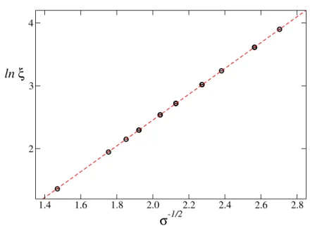
where the logarithmic corrections are taken into account. Note that while Aχis a non-universal amplitude, the coefficient bχ of the leading logarithmic corrections is universal and can be calculated obtaining bχ= π2/16. We now consider the GRPXY model and study the critical behavior of χ and ξ as one approaches the pure XY critical point along the line β = βXY = 1.1199 by decreasing σ. We collected data for 0.46 & σ & 0.14 in the infinite-volume limit, corresponding to the quite large range of correlation lengths 4 . ξ . 50. Fig. 4.3 shows a plot of ln ξ versus σ−1/2. The data fall on a straight line, showing that for σ → 0

ln ξ ∼ σ−1/2. (4.11)

This behavior can be understood within the RG framework. Indeed under general arguments it can be shown that, as long as disorder is less rele-vant than the thermal perturbation, the critical behavior can be simply obtained by replacing τ with the nonlinear thermal scaling field [59]. In fact the thermal nonlinear scaling field utis an analytic function of the sys-tem parameters. Thus, in the presence of disorder it is a function of both 1_{Equation (4.9) holds whatever the definition of the correlation length is, but of}

course X depends on the specific choice for ξ. Reference [64] studied the exponen-tial correlation length ξgap, which is defined as the inverse of the mass gap, and

de-termined the corresponding constant Xgap = 0.233(3). Since in the critical limit [134]

ξ2_/ξ2

gap= r = 0.9985(5), the constant X for the second-moment correlation length we use

is given by X = Xgap√r = 0.233(3).

4.1. CRITICAL BEHAVIOR AT THE PARA-QLRO TRANSITION 1.4 1.6 1.8 2.0 2.2 2.4 2.6 2.8

σ

ln

ξ

Figure 4.3: MC estimates of ξ for β = βXY = 1.1199 and several values of σ

versus σ−1/2_{. The dashed line corresponds to a linear fit to lnξ = Cσσ}−1/2_{+ b.}

τ = (T − TXY)/TXY and σ such that, close to the XY transition point, it behaves as

ut(τ, σ) = τ + cσσ + . . . (4.12) where the dots stand for higher-order terms. If disorder is less relevant than the thermal perturbation, then

ln(ξ/X) = Cu−1/2_t + O(u1/2_t ), (4.13) along any straight line in the T, σ plane which ends at the XY pure transition point. Since this relation also holds for σ = 0 and ut(τ, 0) = τ , C and X are the same constants reported below (4.9). Along the line T = TXY Equation (4.13) implies

ln(ξ/X) = C (cσσ)1/2

+ O(σ1/2), (4.14)

in agreement with the observed behavior. In order to determine cσ we have performed fits to

ln(ξ/X) = Cσσ−1/2(1 + bσ) , (4.15) using X = 0.233(3). We obtain the estimates Cσ = 2.010(2) and b ≈ −0.11. In particular, a fit of the data satisfying ξ & 7 gives Cσ = 2.0102(8) and b = −0.108(2), with χ2_{/DOF ≈ 1.1 (DOF is the number of degrees of} freedom of the fit). Using C = 1.776(4) and Cσ = C/√cσ, we obtain

cσ = µ C Cσ ¶2 = 0.781(4). (4.16)

4.1. CRITICAL BEHAVIOR AT THE PARA-QLRO TRANSITION 2.0 2.2 2.4 2.6 t-1/2 2.0 2.5 3.0 3.5 ln ξ GRPXY CRPXY

Figure 4.4: Plots of ln ξ vs t−1/2_{, where t ≡ (T − T}

c)/Tc, for the GRPXY and

CRPXY models at σ = 0.0576. For both models we use Tc = 0.8528, as obtained

by using (4.19). The dashed line corresponds to a fit of the GRPXY data to ln ξ = ct−1/2_{+ a. The dotted line that connects the MC data is drawn to guide the}

eye.

The constant cσ is non-universal and as such is model dependent. However, for σ → 0 the fields Axy are typically very small and the distribution func-tions for the GRPXY and CRPXY models are identical to leading order in Axy. We thus expect that the first correction to the thermal scaling field due to disorder is identical in the two models, i.e.

ut,GRPXY(τ, σ) = ut,CRPXY(τ, σ) + O(σ2), (4.17) which implies that cσ is the same in the GRPXY and CRPXY models.

4.1.2 C r it ica l b eh av ior of t h e m a gn et ic cor r ela t ion s a t fix ed σ

Standard arguments that apply to critical lines imply that the critical tem-perature at fixed σ must be the solution of the equation

ut[Tc(σ), σ] = 0. (4.18)

Therefore, Equation (4.12) also implies that for small values of σ the critical temperature for the GRPXY model (and also for the CRPXY model if (4.17) holds) is given by

Tc(σ) = TXY[1 − cσσ + O(σ2)]. (4.19) 38

4.1. CRITICAL BEHAVIOR AT THE PARA-QLRO TRANSITION 1.0 1.5 2.0 2.5 3.0

t

ln

ξ

Figure 4.5: Estimates of ln ξ vs t−1/2_{, where t ≡ T/T}

c(σ) − 1, for the GRPXY

and CRPXY models for several values of σ. For σ = 0.0576 we take Tc(σ) = 0.8528

[Equation (4.19)]. For the other values of σ, Tc(σ) is determined from the data.

The lines are drawn to guide the eye. The data for the XY are taken from [135].

Equation (4.19) can be checked by analyzing data at fixed small values of σ. We have performed MC simulations of the GRPXY model at σ = 0.0576 for several values of β, from β = 0.95 to β = 1.02, corresponding to 10 . ξ . 26, and of the CRPXY model at the same value of σ for β = 0.92, 0.95, 0.99 corresponding to 7 . ξ . 16. In Fig. 4.4 we plot ξ versus t−1/2 _with t ≡ T/Tc − 1 and Tc = 0.8528 given by (4.19) [if we take the errors on TXY and cσ into account, we have Tc = 0.8528(3)]. Clearly, ξ → ∞ as t → 0, confirming (4.19). Moreover, they are clearly consistent with the KT behavior

ln ξ = at−1/2+ b. (4.20)

A fit of all available data for the GRPXY model to (4.20) gives a = 1.841(2) and b = −1.511(5) (with χ2/DOF ≈ 1.3) keeping Tc = 0.8528 fixed. A nonlinear fit, taking Tc as a free parameter, gives Tc = 0.852(2), in good agreement with (4.19). Note that the estimate of the constant b is close to the corresponding XY-model value ln X = −1.46(1). This is no unexpected since X(σ) = X + O(σ). We also collected data at σ = 0.1521 for both the GRPXY and CRPXY models, for 0.8 ≤ β ≤ 1.1199 (corresponding to 2 . ξ . 37) and 0.96 ≤ β ≤ 1.145 (corresponding to 5 . ξ . 46), respectively. Again, the data fit well the KT behavior (4.20), see Fig. 4.5. Fits of the MC data for ξ & 10 to (4.20) (for which χ2/DOF < 1) give the estimates Tc = 0.772(2) for the GRPXY model, and Tc = 0.762(1) for the CRPXY

4.1. CRITICAL BEHAVIOR AT THE PARA-QLRO TRANSITION 0.0 0.1 0.2 0.3 0.4 1/lnξ/X 0.6 0.7 0.8 0.9 1.0 1.1 ln χ/ξ 7/4 pure XY GRPXY σ=0.0576 GRPXY σ=0.1521

4.1. CRITICAL BEHAVIOR AT THE PARA-QLRO TRANSITION universal along the thermal paramagnetic-QLRO transition line. Also the slope appears universal (the coefficient bχ does not depend on σ). The constant Aχ corresponds to the intercept of χ/ξ7/4 at ln ξ/X(σ) = 0. As it can be seen from the figure, this constant, which is not universal, varies very little with σ: differences are not visible within our errors, except for the CRPXY data at σ = 0.307. However, note that for this value of σ the critical behavior is controlled by the multicritical Nishimori point, i.e. by the special point M which appears in Fig. 2.1. In conclusion, the above numerical results provide a strong evidence that the magnetic two-point correlations show a KT behavior along the thermal paramagnetic-QLRO transition line in GRPXY and CRPXY models.

4.1.3 Q u a r t ic cou p lin gs

We now discuss the behavior of the quartic couplings defined in (4.5)-(4.7). We recall that in the pure XY model g22= 0 while g4= gc behaves as

g4 = g∗4+ bg

(ln ξ/X)2 + O(1/ ln

4_{ξ), (4.21)}

where g∗

4 and bg are universal. We mention the estimates g4∗ = 13.65(6) obtained by form-factor computations in [135], and g₄∗ = 13.7(2) by field-theoretical methods [136]; other results for g∗₄ can be found in [73] and references therein. In Fig. 4.7 we show some MC results of gcfor the CRPXY model at σ = 0.1521, 0.0576 and the GRPXY model at β = βXY = 1.1199 (within our errors of a few per mille the infinite-volume limit is reached for L/ξ & 10, as in the pure XY model [135]), and compare them with MC results for the pure XY model taken from [135]. The results are identical within errors. For example, if we consider the CRPXY model for σ = 0.1521, a fit to g∗

c + bg/(ln ξ/X)2 gives gc∗ = 13.57(10) and bg = −3.1(1.4), with χ2_{/DOF ≈ 0.4, to be compared with the value [135] g4}∗ = 13.65(6) of the pure XY model. Both g_c∗ and bg, which are universal in the pure-XY universality class, do not depend on σ. The quartic coupling g22 defined in (4.6) is interesting because it is particularly sensitive to randomness effects, since in the pure XY model it vanishes trivially. The estimates of g22 in the GRPXY model for T = TXY and several values of σ are shown in Fig. 4.8. They decrease with decreasing σ, and appear to vanish when σ → 0 as

g22∼ cξ−ε, (4.22)

with ǫ ≈ 1.0. A fit to (4.22) gives ε = 0.97(4), c = 3.1(3) with χ2_{/DOF ≈} 1.1, where DOF is the number of degrees of freedom of the fit. The fast decrease of g22 along the line T = TXY [note that g22 ∼ 1/ξ implies g22 ∼ exp(−cσ−1/2)] might suggest the irrelevance of disorder, and there-fore that the critical value g₂₂∗ vanishes along the thermal paramagnetic-QLRO transition line. This conclusion is apparently contradicted by the

4.1. CRITICAL BEHAVIOR AT THE PARA-QLRO TRANSITION 0.00 0.02 0.04 0.06 0.08 0.10

1/(ln

ξ/X)

g

pure XY

CRPXY σ=0.0576

CRPXY σ=0.1521

GRPXY T=T

c = g∗4= 13.65(6) obtained by form-factor calculations [135].

0.00 0.02 0.04 0.06 0.08 0.10 0.12

1/

ξ

g

GRPXY T=T

Figure 4.8: Estimates of g22versus 1/ξ for the GRPXY model at fixed β = β_XY =

1.1199. The line is a fit of g22to cξ−1.

4.1. CRITICAL BEHAVIOR AT THE PARA-QLRO TRANSITION 0.00 0.02 0.04 0.06 0.08 0.10

1/(ln

ξ/X)

g

σ=0.0576

σ=0.1521

σ=0.2992

4.1. CRITICAL BEHAVIOR AT THE PARA-QLRO TRANSITION

4.1.4 C r it ica l b eh av ior of t h e over la p cor r ela t ion s

We now discuss the critical behavior of overlap correlations, which are the appropriate quantities to understand the role of disorder. We consider the critical behavior of the overlap susceptibility which is expected to behave as χo ∼ ξo2−ηo. In the case of the pure XY model we have ηo = 2η = 1/2. In [58] (see also the previous chapter) it has been noticed that the following relations 2η − ηo≈ σ π for GRPXY, (4.23) 2η − ηo ≈ σ +1₂σ2 π for CRPXY (4.24)

approximately hold in the whole QLRO phase (within the small statistical errors), even very close to the KT transition, as long as σ is not too large (in practice σ should not be close to σM, where M is the Nishimori point defined in Fig. 4.2). This would suggest that they may remain valid up to the transition. Given the strong numerical evidence that the exponent η as-sociated with the magnetic correlation is η = 1/4, the above relations imply that ηo varies along the paramagnetic-QLRO transition line approximately as ηo ≈ 1 2− σ π for GRPXY, (4.25) ηo≈ 1 2 − σ + σ2/2 π for CRPXY, (4.26)

at least for sufficiently small values of σ. We wish now to verify if the high-temperature data are consistent with these predictions. In Fig. 4.10 we plot χo/ξ2−ηo versus 1/ ln(ξ/X). The scaling is reasonable. We also report χo/ξ2−ηo, fixing ηo to the pure XY value ηo = 1/2. Again the ra-tio is consistent with a limiting finite value. However, if χo behaves as in the pure XY model, we would expect a σ-independent slope, which is not supported by the data. We now consider the ratio ξo/ξ between the second-moment correlation lengths obtained from the overlap and spin correlation functions. 2 In order to estimate this ratio in the case of the pure XY model, we performed MC simulations (using the Wolff cluster algorithm) in the range 0.93 ≤ β ≤ 1.033 corresponding to 12 . ξ . 110. Taking into account the logarithmic scaling corrections, i.e. fitting the XY-model data satisfying ξ & 32 to a + b/(ln ξ/X)2 with X = 0.233, we obtain the estimate ξo/ξ = 0.417(4). In Fig. 4.11 we show the results for several values of σ. They are all consistent with a finite critical value, confirming that the paramagnetic-QLRO transitions are characterized by a single diverging 2_{In a Gaussian theory without disorder, in which the magnetic correlation function is}

given by eG(p) = (p2_{+ m}2₎−1_{, one can easily find that ξ} o/ξ =

p

1/6 = 0.408248... 44

4.1. CRITICAL BEHAVIOR AT THE PARA-QLRO TRANSITION 0.0 0.1 0.2 0.3 0.4 0.5 1/ln ξ/X -0.4 -0.2 0.0 0.2 0.4 0.6 ln χ o /ξ o ε pure XY GRPXY σ=0.0576 GRPXY σ=0.1521 GRPXY σ=0.1936 CRPXY σ=0.1521