Università degli Studi di Messina
Dipartimento di Scienze Matematiche, Informatiche, Fisiche e
Scienze della Terra (MIFT)
Dottorato di Ricerca in Fisica
XXXI Ciclo
Drawing up, development and optimization of
a Limited Area Model for meteorological
forecasting in regions with complex
orography
PhD Student
Dr. Giuseppe CASTORINA
Supervisor:
Chiar.
moProf. Salvatore Magazù
Introduction
The global climate changes and their impact on global scale represent one of most important issues nowadays. In the recently years, the understanding of the climate changes, through the studies of ice ages and interglacial ages have intrigued many scientists and researchers. Studying the last million year, they found that with a periodicity ranging between 40 and 100 thousand of years, there was a average temperature fluctuation of 10 K. Assuming the average temperature of the earth as a fundamental variable and disregarding the contribution of the atmosphere, through the global energy balance theory, one has:
𝐶𝑑𝑇
𝑑𝑡 = 𝑃𝑖𝑛− 𝛼𝑃𝑖𝑛− 𝑃𝑜𝑢𝑡
where C is the heat capacity of the Earth, and Pin is the incoming radiation given by Pin = πR2S. Pin it is independent on Earth’s temperature but affected by the time as function of astronomical modulations. In the last relation, S ≃ 1370Wm−2, is the solar constant and πR2 represents the surface perpendicular to the solar rays. Pout is the emitted radiation by the surface of the Earth estimated through the Stefan-Boltzmann law for the black body at T temperature: Pout = 4πR2σT4 (σ ≃ 5.67 × 10⁻⁸Wm−2K−4 Stefan-Boltzmann constant). Finally, α is the average albedo of the Earth (typically of the order to 0.3).
The climatic fluctuations are related with the astronomical variations of the terrestrial orbit (cycles of Milankovitch), but at global level, the variations of insolation alone can not explain the variation of 10 K observed in climate data. Therefore, an amplification mechanism to move from small solar modulation to the great climate change, it is necessary. According to G. Parisi [1], this mechanism is governed by positive feedback induced in the albedo. A further amplification is due to stochastic resonance induced by the weather fluctuations. When treating with physical phenomena that involve variables with different time scales, it is possible to consider the faster ones as perturbations acting on the slower.
The study of the climate: climatic fluctuations
From the examination of several different elements, direct and indirect, it has been possible to form an indicative picture of what has been the climate of the earth in the last decades, in the centuries, in the millennia and in the geological epochs. During the last two million years there have been alternations between periods of glacial climate and less cold (interglacial) intervals with periods of ice ages of about one hundred thousand years. On the basis of these elements, it appears that the
climate is subject to variations that have different time scales, also highlighting that the evolutionary trend of the long-term climate is completely masked by relatively short period fluctuations and therefore imperceptible.
What are the physical causes of climatic fluctuations?
A first hypothesis is that they can occur within the same climate system without the intervention of external factors. In fact, there are many mechanisms that can give rise to an internal variability of the system. This derives from the non-linear interactions (called "feedback") that occur between the various parts of the complex, which have very different reaction times.
A typical mechanism of this kind, which binds together the snowpack, the reflection of the radiant energy of the sun and the temperature of the air, could be the following: suppose that a small decrease in temperature occurs, such as to favor the extension of the snow cover on the Earth, the increased reflection of solar radiation by the snowpack would further reduce the temperature, thus hindering the sun's warming of the earth's surface.
Other climate influences may result from changes in the amount of particulate matter in the upper atmosphere due to volcanic activity, or an increase in the carbon dioxide content in the air as a result of fossil fuel fires.
An example of the possible effects that volcanic eruptions could have on climate fluctuations occurred in 1816, the year following the eruption of the Tambora volcano, on the Sumbawa island of present-day Indonesia (then the Dutch Indies), which took place from 5 to 15 April 1815.
The summer of the 1816 is remembered as the coldest recorded in the previous 200 years, in various parts of Europe, in the American states of the northeast and in eastern Canada. The cause of this anomaly seems to lie precisely in the enormous quantity of powders poured into the high atmosphere of the volcanic eruption, greatly increasing the reflectivity of the atmosphere towards the incident solar radiation. In this regard, it should be recalled that recently two researchers from NCAR in Boulder in Colorado observed that changes in the amount of particulate matter in the upper atmosphere are a better indicator than the number of sunspots to determine temperature fluctuations. Another question that fascinates the man is as follows:
Can human activities on Earth be the cause of current or future climate changes?
That the climate is affected by urban areas is, for example, a proven reality: "the heat island" at the cities is a well documented fact that affects areas of the order of one thousand square kilometers. These influences, however, are of a purely local character and are presumed to have no relevance to the general climate of the earth. The problem is another: the increase in the use of fossil fuels, from the end of the last century to the present, has led to an increase in atmospheric carbon dioxide (C02) by 10% and is such that if by one or two centuries all available fuel reserves were consumed, the
concentration of CO2 in the atmosphere would increase considerably. It is presumed that this could give rise to a significant increase in the temperature of the earth with appreciable consequences on the other elements of the climate.
Fig. 1: Graph showing the increase in CO2 over the years
Is it possible to make any predictions about the future evolution of the earth's climate?
Although much progress has been made in recent years towards the development of a quantitative climate theory, both through experimental and observational studies and through mathematical models, science is not yet able to provide a reliable answer. Some indications can be deduced with statistical methods taking into account the possible future implications of human activity. Climate fluctuations in the past seem to suggest that the interglacial warming of the last eight thousand years should be replaced by a cooling regime. The start of this turnaround could still be a few hundred years away, or even already in progress: the gradualness of the phenomenon would be such as to make the variation imperceptible for periods of the order of years. It should be kept in mind that the previous statement may not be valid if, as has already been mentioned, the increase of carbon dioxide in the atmosphere prevails, together with other effects. If this second hypothesis were to come about, there would be a considerable reduction of ice on the Arctic regions, with important consequences for the climate of the whole globe.
In conclusion, it seems necessary to make every effort to progress in the schematization and representation of all the factors and all the possible mechanisms of interaction between the various parts of the system, with particular reference to the atmosphere - ocean exchanges. These studies should be integrated with worldwide measures of several elements, including:
• Average CO2 content, nitrogen oxides, tropospheric aerosols, etc .; • Reflective powers of the earth's surface, especially of snow and ice.
With these measures it will be possible to compare hypotheses and theoretical schemes with the observed experimental data.
Global warming and Extreme Meteorological Events in Sicily
Climate changes such as the global warming, are important not only from a scientific point of view. They can have implications also in social, economic and political environments. In fact, on December 2015 (Paris) at the United Nations conference on climate change (COP21) has been decided that before the end of century the global warming must be kept less of 2 °C.
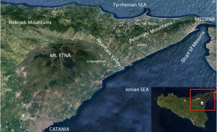
During this meeting was discussed about the area known as “Stretto di Messina” which is one of most interesting area from climate point of view.
Fig. 2: The image shows the circulation of water masses in the Strait of Messina, between Calabria and Sicily. The strait has the reputation of being among the most unstable seas in the world
Its complex orography, the clash between the Ionian and Tyrrhenian seas, which have completely different kinds of salinity, temperature and density but also the exposure to winds both from northern quadrants and southeast, make this area among the most unstable of the world. Further, statistically
this area is interested by extreme weather events which often produce considerable property damage and sometimes loss of human lives.
The year of 2016 has been registered a new negative record. In particular, this year results as the most warm ever registered (NOAA: National Oceanic and Atmospheric Administration).
Fig. 3: Temperature anomalies of 2016 (source NOAA)
But the significant increase in planetary temperature has led to an increase in the frequency of extreme events in the “local area”?
In recent years, a growing attention has been addressed to environmental issues due to the significant increase registered, both in the number and intensity, of extreme weather events. The attention of stakeholders on phenomena as flash floods, strong winds and heavy seas has grown also as a result of the impact on daily life caused by landslides, damage to buildings and to agriculture and, in the most tragic circumstances, to the loss of lives. It clearly emerges, therefore, how important is the prevention of these phenomena. This can be performed only through an accurate study of the physical causes which determine such events. It clearly emerges the necessity to invest resources in the field of meteorology, to implement and improve the performance of forecasting bulletins, to broaden the detection network making it as dense as possible, to boost research in the field of weather numerical modeling, and to set up a sufficient number of operation unities connected with weather civil services. From a general point of view, heavy rainfall events in the Mediterranean can be divided into two types: floods and flash floods. The “Floods” are due to intense and long lasting precipitations (often
of several days) caused by the decrease of atmospheric circulation on a given area. The “Flash floods” are phenomena which consist in heavy and short precipitations (e.g. 60 mm/hour), where, even in 3 - 4 hours, pluviometric accumulations that are usually detected in an entire season can be recorded [2]. On the other hand, from the specific analysis of the extreme precipitation in Sicily, it emerges that the precipitations are nearly always connected to the action of particularly intense storm cells. These systems are usually divided into single cell storms and multi-cell storms [3]. The single cell is characterized by the presence of a single cumulonimbus (cloud with a pronounced vertical development), that has an average life time of 15 - 20 minutes and, therefore, has a low probability of initiation of flash floods. Furthermore, in the single cell storms, it’s easy to determine the direction of motion, characterized by a displacement which follows exactly the level guides, the wind at 500-hPa level.
The mechanism that regulates the structure of a multi-cell system is quite different and more complex; in fact, the multi-cell is characterized by a regeneration process triggered by the cold downdraft (gust front) of the mature cell. This can lead to the development of a cluster of 3 - 4 cells that, therefore, would have a mean lifetime of about 60 minutes. In this case the displacement of the system does not follow the level guide but its direction is obtained from the sum between the average wind speed at 850 - 700-500 and 300 hPa and the vector opposite to the flow at 850 hPa that with the gust front will generate new cells.
By taking into account the length of the time-window that these weather perturbations can achieve, they can become cause of storms.
Among the mesoscale convective systems which can result in flash floods, one can distinguish:
MCS (Mesoscale Convective System), in linear form if produced by cold front or circular in the case of cold drop;
MCC (Mesoscale Convective Complex) which is a set of MCS or a MCS very wide. This system, characterized by a temperature of the convective core less than -52 ° C of at least 50,000 km2, and by a surrounding crown with temperatures lower than -32 ° C for at least 100,000 km2 [4].
However, the thunderstorm system potentially dangerous for the Mediterranean, and in particular on Sicily, is the so called "V Shaped” storm. Analyzing the causes that lead to its formation is equivalent to predict, in advance, favorable conditions to the manifestation of extreme events, such as those that occurred in eastern Sicily. The origin that give rise to the formation of very intense storms are to be linked to the presence of "deep instability" conditions that are to be found in the temperature and
humidity profiles in the air column of the arrival mass and in the existing site as well as the interaction between air masses of different nature thermo-hygrometer [5]. In the analyzed cases very often at the same time were observed:
high amount of water vapor provided by the "warm conveyor belt" (a kind of river of warm and humid air flowing in the lower level troposphere in correspondence with the warm sector, namely between the rear of a warm front and the front of the cold front which follows) estimated by ThetaE (equivalent potential temperature or pseudopotential, namely the final temperature of a particle flow rate from a reference dimension, in this case 850 hPa, the conventional 1000 hPa ) values that quantify the contribution of moist air;
extensive resources of thermal energy (latent and sensible heat supplied from the sea) for strengthening updraft (hot running upward) [6];
diffluence of jet stream flowing between the isobaric surfaces of 500 hPa and 300 hPa or - alternatively - jet streak (jet “core”, which is the maximum speed of the jet stream) transit; diffluence in the high troposphere level (the rate of the change of the direction of the flow in
the direction transverse to the motion); convergence lines to low level (often for the presence of a minimum baric secondary), nuclei of positive vorticity;( 2ω, with ω the fluid angular velocity, it is positive in case of counterclockwise rotation (cyclonic));
stronge vertical wind shear (evidenced by the presence of a sub-tropical jet stream at 300-hPa level ;
strong veereing of the wind with height, with southeasterly low flow underlying southwesterly flow aloft;
high values of Convective Available Potential Energy: CAPE high thermodynamic indices such as LI, K, TT, PWAT, SREH;
orographic forcing that can generate dynamic feedback to persistent thunderstorms produced by the self-regenerating convective cell along the coast (cold air, after the precipitation, slides down the slope can generate a mini cold front (gust-front) on marine waters overlooking the mountain range, triggering a new convective activity)
in some cases "dry intrusion", i.e. the intervention of a corridor of very dry air at the isobar of 500 hPa surface (the cold and dry air is heavier than warm and moist, therefore, if present at high altitude, is destined to sink to the ground which allows to trigger, animate, or possibly, intensify the convection)
Although a thorough analysis of these conditions can help estimate the likelihood of an extreme phenomenon and its location, it is appropriate to careful monitoring and forecasting very short-term
(nowcasting through satellite and radar) after the formation of the same, in order to identify the trajectory and, therefore, the areas that will be invested, in addition to his stage of development (next attenuation or intensification, evaluated on the basis on the energy of the system) [7].
In order to evaluate the probability of the genesis of storms it has been calculated the thermodynamic index CAPE [8], which measures the energy gained from the floating air mass until, during the ascent, remains warmer environment air. In other words, the CAPE measure the work done by the buoyancy and its unit of measurement is J / kg. For example, the CAPE of 1500 J / kg implies that a package of air of 1 kg has received, during the rise, a total energy of 1500 J. Under certain conditions and in the absence of interactions with the external environment and / or turbulence, (assuming that the parcel ascends without mixing with the environment) this potential energy is converted entirely into kinetic energy, going to animate intense updrafts. It’s precisely the maximum kinetic energy available to convective systems which determines the intensity of the vertical speeds of the air mass and, hence, in the case of values of relative humidity near to 100%, the precipitation.
Extreme weather events are characteristics of the Mediterranean coastal areas and often cause flash floods. During these episodes, the precipitations that occur in a few hours often exceed the rain accumulations that normally occur in several months [9].
Usually, these extreme precipitations are in conjunction with intense and quasi-stationary mesoscale convective phenomena that insist on the same area for several hours [10]. Local factors such as the presence of orographic reliefs along to the coastline often determine their intensity. The geographical position and the complex orography of Sicily often cause extreme weather events [11-12]. Positioned at the center of the Mediterranean Sea, the island is placed in the transition zone between the arid and dry climate of North Africa; the more temperate and humid climate of central Europe. Hence, the phenomena trigger the interactions between processes typical of middle latitudes and the tropics.
In early autumn, the Mediterranean cyclones that originate from the contrast between air masses with very different temperatures and humidity interacting with seawater high temperature (Sea Surface Temperature, SST), affect the seas surrounding Sicily. These conditions can cause extreme weather events characterized by sudden and heavy rainfalls and dangerous flash floods [13].
From the geographic point of view, Sicily is characterized by an orography distributed in the direction of the parallel, especially in the Northern area, which is strongly exposed to the atmospheric perturbations that come from the South. In such cases, the warm and moist air coming from the Libyan Sea is often lifted over the orographic barriers, losing its humidity because of the cooling, and these modifications can cause heavy rains [14-15]. This occurs especially in the autumn seasons when the
sea around the island is still warm and able to transfer large amounts of humidity into the atmosphere [16-17].
It clearly emerges that the island complex orography plays a key role in the portion of the Ionian coastline between the towns of Catania and Messina.
Recently, extreme weather conditions have affected the eastern coast of Sicily, in particular the area between Catania and Messina. For example, from the tragic sequence of severe meteorological events that occurred between 2007 and 2011 in the below towns:
25 October 2007, which took place at Santa Margherita, Giampilieri and Scaletta (Messina), with flash flood and precipitations of 175 mm in 2 hours, against an annual average amount of 800-1000 mm;
01 October 2009 at Giampilieri, a tragic and disastrous event with 37 victims.
22 November 2011 at Barcellona and Saponara (Messina) with precipitations of 351 mm in 10 hours (recorded by the Castroreale weather station);
Referencing these three events, the recovery costs of the disaster damages were estimated at about 900 million euros (Source: DRPC Sicily – Stato dei rischi del territorio Siciliano – Rischio idrogeologico: raccolta dati storici – Sicilian Territory State of Risk – Hydrogeological Risk: Historical data Record).
Analysis of pluviometric accumulations in Sicily from 2002 to 2014
A study conducted by Sias (Servizio Informativo Agrometeorologico Siciliano) in 2010 showed [18] that rainfall accumulations of the Sicilian Region, in the period from 1921 to 2001, showed a downward trend average of about 19mm / decade.
But this trend appears to be confirmed? The increasing of the extreme weather events should not lead to a significant increasing of rainfall?
Table 1: Values of annual precipitation collected by agrometeorological Sias stations. NB: Red cells highlight the data below the average temperatures expected. The column " Climate " is the average value of
the rainfall of the last thirty years;
The row " Sicilian average" was calculated by averaging arithmetic value
precipitation of the individual years of nine Sicilian provinces: Trapani (TP), Palermo (PA), Messina (ME), Caltanissetta (CL), Agrigento (AG), Catania (CT), Enna(EN), Ragusa (RG), Siracusa (SR).
In the Table 1 the values of annual precipitation observed at 107 agrometeorological stations of Sias located throughout the region Sicily, are reported [19]. The source data has been provided by Sias and the meteorological parameter investigated is the "daily precipitation total - monthly total" (in mm).
The table has been realized as follows:
1. After having cataloged stations for provinces of belonging, it is calculated for each station the "sum of annual precipitation values" registered a monthly basis;
2. It has been estimated the average annual rainfall of the stations belonging to each province, resulting in the "average annual rainfall provincial" in the table.
Fig. 4: Sicilian annual average rainfall obtained through provinces average.
Blue dots: values of annual average precipitation in Sicily; magenta continuous line: Sicilian climate average of the last thirty years
Fig. 5: Province annual average rainfall.
Blue dots: values of annual average precipitation in each Sicilian province;magenta continuous line: climate average of the last thirty years of each Sicilian province.
By the analysis performed, it emerges that, as shown in the Fig. 4, for the year 2002 an average Sicilian below the climatic averages has been registered; from 2003 to 2014, except the year 2008, it emerges a substantial increase in average rainfall in Sicily. In Trapani, Messina, Catania, Ragusa and Siracusa have been registered the largest increases, as reported in the Fig. 5.
The increase in global temperature and the surface of seas raises the probability of generation of extreme weather events such as heavy rainfall: this leads to the reversal of the trend of rainfall which is therefore growing [20-22].
The intensity of the convective systems can be increased by high resources of thermal energy in the lower layers [23].
In the last 150 years the average temperature on earth has been a gradual increase; the Global Warming has reported a sudden acceleration since 1980.
Fig. 6: Global land – ocean temperature index
Nowadays a great debate about the causes, whether natural or man-made, which have led to an increase in the average temperature of the Earth, of about 0.8 ° C in the last thirty years, is in progress [24]. It is clear that the two hypotheses should not be in close antithesis since the effects of the two causes may overlap. Increased concentrations of greenhouse gases, caused by the action of human activities (CO2 in the atmosphere up to 386ppm against the value of 270 of the pre-industrial period), would have resulted in a substantial overheating. Such gas, in fact, is retained in atmosphere: soil
heating by radiation shortwave, cooling for reintroduction long-wave (infrared) inhibited by the presence of gas called - precisely - "greenhouse"[25].
Another hypothesis invoked to justify the rising temperatures in our planet, formulated by researchers of the Earth Institute at Columbia University (http://earth.columbia.edu/news/2003/story03-20-03.html) deals with a significant variation in solar activity, that has been gradually increasing in recent years.
Beyond the actual cause of Global Warming, the significant increase of the planetary temperature, has led to an increase in the resources of thermal energy available for convective phenomena, and, hence to an increase of the evaporative potential of seas and, consequently, to a rise in the frequency of extreme events.
The increasing of the global temperature and of the surface of our seas determines raises probability of generation of severe weather events such as heavy rainfall: this leads to the reversal of the trend of rainfall which is therefore growing.
This, in theory, would favor an increasing of the rainfall. The analyzed data confirm this trend: in Sicily, from 2003 to 2014, with the exception of 2008, there were accumulations rainfall higher than average weather.
Weather Station-Arduino Interfacing for a Weather Monitoring System
Programmed for Emergency Weather Conditions
The significant increase of extreme weather conditions generates more and more concern. In fact, it is full-blown, that phenomena such as flash floods, strong winds and storm surges cause relevant impact on everyday life: landslides, mudslides, and damage to buildings and agriculture and, in the most tragic cases, loss of life. As a rule, the predictability degree of the emergency weather conditions can be often quite low because it is very difficult to go into the exact space-time location of particularly heavy rainfall of limited extent. Weather conditions [26], which can raise the risk level of extreme events, are well known by the operators that know local orography and have experience about territory response to a particular type of “stress”. This often requires a depth and careful study of the physical causes (analysis of thermodynamic variables and atmosphere’s dynamics) that are involved in the genesis of these events. It is equally important, indeed essential, to strengthen the networks of detection in the area of interest, making them more capillary as possible and equipping each station with the necessary technology for real-time data transmission for 24 hours on 24 now-casting (immediate future forecasts, until a few hours). An accurate short-term weather forenow-casting system for a preventive warning, that uses a network detection of high spatial resolution, can be very useful. A recent example of extreme weather condition in Sicily is that of 10th October 2015. The highest rainfall accumulations were recorded on the Ionian sector of the province of Messina. The SIAS station in Antillo (not equipped with alarm systems) recorded 223 mm in a few hours; an extremely high amount of rain in the unit of time that was directly responsible for the flood wave of the Mela Torrent, whose overflowing gave rise to the flooding registered in the territory of Milazzo and Barcellona Pozzo di Gotto. In these municipalities, small rainfall accumulations were recorded (about 10 - 20mm). For this reason critical hydrogeological situations were not expected.
Such extreme events occur in the presence of Mediterranean cyclones, in the pre - frontal phase and in the hot sector of the depression system. Especially in the first phase of the autumn season we often witness the transit to a large series of cyclonic vortexes that, in rapid succession, often in formation due to orographic causes on North Africa (leeward to the Atlas range) or in the Balearics (leeward to the Pyrenees) and then pushed on the central Mediterranean by the ascending branch of the Sub-Tropical Stream, they reach our region. Having entered the Mare Nostrum, characterized by much higher surface temperatures than the oceanic ones, these cyclonic vortexes, fed from below, acquire the huge resources of thermal energy (water vapor and sensitive heat).
In this case, on the night between October 9th and 10th 2015, the low pressure center, moving between Tunisia and our region, activated an intense flow of southern currents, recalling from the Libyan coasts a rather hot air mass (even 25 ° C in the isobaric surface of 850 hPa, or at an altitude of 1520 m elevation). The strong winds of Scirocco in the low strata, in contact with the sea surface, in the stretch of sea between Libya and Sicily, caused an increase in the relative humidity of the air mass of
North African origin, accompanied, therefore, by very high values of the equivalent potential temperature in the lower layers. The "potential energy available for convection" (CAPE) reached peaks even higher than 4000 J / kg on the seas south of Sicily. This heat reservoir, ready to be converted into kinetic energy, or in strong upward currents, was triggered by the initial, apparently mechanical lifting of the hot air layer next to the ground. The reliefs exposed to the Scirocco winds, ie the eastern ones, and in particular the Etna and the Peloritani, favored the forced ascent of the hot and humid air mass directed towards Sicily. During the morning of October 10, our region was affected by a remarkable cumuliform activity that, thanks to a marked vertical "wind shear", due to the strong Scirocco on the ground and the south-western currents in the immediately overlying layers, generated storm cells also particularly intense in the area between Messinese Ionian and the eastern side of Etna. The mathematical models on a global scale, on that occasion, did not propose values worthy of note in the field of precipitation.
It is clear, therefore, because the storm cells are often of an extremely limited extension, only the real-time weather station data transmission can provide an alert system on a very precise location. In this way, weather stations, specifically programmed, located in strategic risk areas, such as streams’ sources, where are recording critical meteorological parameters (such as severe rainfall amounts, wind storm, etc.), can send an alert message to the weather experts and/or authorities in order to be able to set up and carry promptly procedures to alert population.
Weather station/Arduino monitoring system
The data acquisition system is composed by a LSI LASTEM weather station, integrated by an Arduino YUN for the remote connection, able to capture typical meteorological parameters such as rainfall, wind speed, wind direction, temperature, relative humidity, solar radiation and barometric pressure [27].
The employed weather station consists of a 12 inputs data logger, a sensors kit and a software for acquisition programming and data transfer and an Arduino YUN for the remote connection. In addition, weather sensors, such as:
- DNA202 sensor is a speed wind meter, characterized by compact size and a robust structure and of rotor and it is suitable to acquire low and high speeds up to 75 m/s. The sensing element is a high efficiency and durability relay-reed. The sensor body is made of anodized aluminum, while the rotor is made of carbon fiber reinforced;
- DNA212 sensor is a direction wind meter; it is very compact, sturdy and suitable both in very low and strong wind conditions; it is up to durability applications without maintenance. The measuring element is a Hall Effect transducer and the sensor body is composed of anodized aluminum. The above two sensors are completed of a cable L= 3m with connector IP65; - temperature and relative humidity sensor is a thermos-hygrometer. It is specifically dedicated
to meteorological applications where there may be rapid thermo-hygrometric variations and there may be long periods of hygrometric saturation. An anti-radiation shield protects the sensor from solar radiation by ensuring the best accuracy of the temperature measurement; - barometric pressure sensor has an accuracy of 1hPa; it is housed in the IP65 box, where the
data logger is fit;
- solar radiation measurement sensor obeys the requirements of Class 2 of the standard ISO9060 and specific WMO No. 8; it is lightweight and compact;
- rain gauge is characterized by an exterior part of anodized aluminum. The measurement system consists of a collector cone and a teeter connected to a magnet, which activates a reed relay, each teeter corresponds to 0.2 mm of rain. The rain gauge is mounted on a base positioned on a flat surface.
Power supply is a key component of this system, because a continuous power supply is necessary to make the system work continuously. A rechargeable battery is connected with a solar panel. The heart of the system is the data logger in which the values are stored. The E-Log data logger, allows the signals acquisition from the meteorological sensors, the processing and the storing of statistical values and the typical calculations of the weather applications with a particularly low power consumption. The Arduino YUN board is connected to the weather station with the E-log.. It is a microcontroller board based on the ATmega32u4 and the Atheros AR9331. The Atheros processor supports a Linux distribution based on OpenWrt named Linino OS.
Fig. 9: Arduino YUN board.
LSI-lastem weather-station and Arduino YUN interfacing
Arduino YUN board connects the LSI-Lastem weather station to E-log sending real-time data weather at a control center to emergency weather conditions monitoring. The RS232 cable of the weather station E-log is connected through an USB/RS232 adapter to the YUN MicroUSB port. The measures taken by the weather station sensors are sent from E-log through the USB port to the Arduino board, which then sends the measurements via Internet to the Cloud. The YUN distinguishes itself from other Arduino boards in that it can communicate with the Linux distribution onboard, offering a powerful-networked computer with the ease of Arduino. In addition to Linux commands like cURL, it is possible can write your own shell and python scripts for robust interactions.
The Bridge library facilitates communication between the two processors, giving Arduino sketches the ability to run shell scripts, communicate with network interfaces, and receive information from the AR9331 processor. The USB host, network interfaces and SD card are not connected to the 32U4, but to the AR9331, and the Bridge library enables the Arduino to interface with those peripherals.
Fig. 11: Arduino YUN Block Diagram.
In terms of Communication, Arduino YUN has a number of facilities for communicating with a computer, another Arduino, or other microcontrollers. The ATmega32U4 provides a dedicated UART TTL (5V) serial communication. The 32U4 also allows for serial (CDC) communication over USB and appears as a virtual com port to software on the computer. The chip also acts as a full speed USB 2.0 device, using standard USB COM drivers. The Arduino software includes a serial monitor, which allows simple textual data to be sent to and from the Arduino board. The RX and TX LEDs on the board will flash when data is being transmitted via the USB connection to the computer. Digital pins ‘0’ and ‘1’ are used for serial communication between 32U4 and AR9331. The communication between the processors is handled by the Bridge library. A Serial library Software allows serial communication on any of the YUN’s digital pins. Pins ‘0’ and ‘1’ should be avoided as they are used by the Bridge library. The ATmega32U4 also supports I2C (TWI) and SPI communication.
On the SD card of the board, the Node.js (a JavaScript environment that allows user to write web server programs), is installed. Below, it will be used to connect a microcontroller to a web browser using the node.js-programming environment, i.e. HTML, and JavaScript. Node Serial port Library to communicate with serial port of E-log is installed. It allows serial communication on any YUN’s digital pins. Pins ‘0’ and ‘1’ should be avoided as they are used by the Bridge library. In the JavaScript
file (named serial.js) the parameters and protocol communication, send/receive commands controls are specified. “A1I\r\n” command is sent to log, as a string, in TTY communication protocol, E-log responds by sending a string containing all the measurements of the sensors of the weather station. Making a parsing of the string, is possible to get the weather station measures.
Communication parameters are: - Baudrate = 9600 bps; - DataBits = 8; - Parity = ‘none’; - StopBits = 1; - FlowControl = false.
The program code of serial.js is:
/* serial.js */
var serialport = require("serialport");
var serialPort = new serialport.SerialPort("/dev/ttyUSB0", {baudrate: 9600, dataBits:8, parity:'none', stopBits: 1, flowControl: false, parser: serialport.parsers.readline("\n") }); serialPort.open(function (error) { if ( error ) {
console.log('failed to open: '+error); } else { //open connection serialPort.write("A1I\r\n", function(err,result) { console.log('error: '+err); });
var interval = setInterval(function() {
serialPort.write("A1I\r\n", function(err,result) { console.log('error: '+err); }); },10000); serialPort.on('data', function(data) { //console.log(data.toString()); console.log('\n'); try { var values=data.split(";");
console.log('Wind Direction: '+values[0].toString()); console.log('Power Supply: '+values[1].toString()+ ' V ');
console.log('Internal Temperature: '+values[2].toString()+ ' \u00B0C '); console.log('Wind Speed: '+values[3].toString()+ ' m/s ');
console.log('Air Temperature: '+values[4].toString()+' \u00B0C ');
console.log('Relative humidity: '+values[5].toString()+' %'); console.log('Rainfall Accumulation: '+values[6].toString()+' mm/h'); if (values[3]>25.0) { console.log('ALERT WIND'); } if (values[1]<11.0) {
console.log('ALERT POWER SUPPLY'); } if (values[6]>30.0) { console.log('ALERT RAIN'); } } catch(err){ console.log('waiting...'); } }); } });
Typing “node serial.js” into Linux shell will appear as the result shown in the Fig. 12:
Fig. 12: Typing “node serial.js” into Linux result window.
The program sends weather warnings (in the case in which the measure Rainfall Accumulation is greater than 30 mm/h or in the presence of strong wind with wind speed greater than 25 m/s) and a warning message relating to an insufficient power supply.
The WRF model
The Numerical Weather Prediction
The Numerical Weather Prediction (NWP) represents one of the most complex challenges of Atmospheric Physics. The objective of knowing in advance the evolution of time with a reasonable degree of reliability can now be pursued thanks to the development achieved by modern computers. The parallel development of the computer networks and the internet has made the weather forecast available at a capillary level thanks, for example, to the usability of specific applications on multiple communication devices. However, it should be stressed that the above-mentioned weather data diffusion, while meeting the sharing requirement, if not properly filtered, does not guarantee the correctness of the information itself.
Definition of model and of the main constituent equations (primitive equations)
From a general point of view, a meteorological model is nothing but a schematic and simplified representation of physical reality, described through a set of equations that simulate the behavior of the atmosphere. A particular software uses input data, executes a run using algorithms based on a set of coupled equations, and expresses the output result (output) in the form of a new set of data. In the case of meteorological forecasting, the calculation algorithms consist of the set of differential equations to partial derivatives, which describe the dynamics of the atmosphere. The main core of a calculation code aimed at solving this system of differential equations is normally formulated in FORTRAN language. Specific subroutines, such as those related to matrix processing, to standard mathematical functions and to graphic sections, can use other languages, usually C.
As input data of the model, the values of: ground pressure, wind speed in its spatial components, air temperature and humidity at different altitudes of the atmosphere (up to about 20 ÷ 50 km in height) are usually used. These variables, called Ap prognostic variables, are present in the model in the form of derivatives with respect to time 𝜕𝐴𝑝
𝜕𝑡
.
These variables play a key role within the model because they coincide with the variables object of the observations and because in the progress of the calculation they allow to derive also all the other variables that depend on them, called diagnostics. The goal of a forecast is to return, after the calculation, the mutated value of the above-mentioned variables (i.e wind speed, temperature, pressure, humidity at various heights from the ground). From these you can then derive all the other dependent quantities: precipitation, cloudiness, etc ...
The main equations, called primitives, which are used by the models are:
Navier-Stokes (NS) equations for the definition of wind field components (also called momentum balance equations in a fluid);
First Principle of thermodynamics (principle of conservation of energy);
Equation of evolution of water vapor (takes into account all the processes that make up the water cycle and its state passages, ie evaporation, condensation, fusion, solidification and sublimation);
Continuity equation (mass conservation law). To these equations are added:
Gas state equation, which binds pressure, density, temperature and volume of a mass of air. Hydrostatic equation, which concerns the approximate relationship between pressure
variation with altitude and air density.
Global models and limited area models
There are two types of meteorological models: Global Models (GM) and Limited Area Models (LAM). It is intuitive that global models take into account the whole earth's atmosphere, while those with limited area operate on smaller volumes. Since there are no simple analytical solutions of the system of equations valid for all points of the atmosphere, it is necessary to resort to a partition of the portion of the atmosphere of interest, in a three-dimensional matrix identified by grid points, thus reformulating the problem in discrete terms, once the boundary conditions have been defined. The simplification adopted, which takes the name of discretization, implies that the derivatives are replaced by finite differences.
This substitution makes the original differential equation system suitable for numerical calculation. This approach involves the definition of a series of fixed points, selected in the domain of definition of the equation variables. Each variable is then completely identified by the values assumed on these points, the so-called grid points, while the spatial derivatives become finite differences evaluated between the grid points. It should be noted that at each grid point a portion of atmosphere is associated, whose characteristics are represented by the values assumed by the variables. Therefore, the forecast becomes a procedure for calculating the future values of the meteorological variables on all grid points. In the specific case, one imagines to completely dissect the atmosphere both horizontally and vertically by means of a three-dimensional grid of appropriate scale. There are no constraints on the total number of points (also called nodes) to be used, although it is evident that by
infilling the grid the interval between the points decreases and this results in a better precision of the numerical computation. In practice it is the computing power of the electronic instrument that limits the choice of points: either the whole globe is considered and therefore the distance between the nodes is kept wide, or one concentrates on an area by infilling the grid step, thus gaining in resolution. Since the automatic calculation capabilities are finished, the Global Models, having the largest grid pitch, introduce the most important simplifications, operating with resolutions between 10 and 50 km horizontally.
The LAM, reducing the area of interest, use a denser grid, with a typical pitch of 1 ÷ 10 km. In vertical, the portion of the atmosphere considered can extend up to a height of 30 ÷ 70 km, distributed on about fifty levels, in an uneven way (denser near the ground, where a better vertical definition is required). It is important to underline that the Global Models serve to initialize the LAM, that is, at the initial instant t = 0 relative to the beginning of the calculations, the LAMs use the GM outputs as initial values and then elaborate a prediction.
In addition, GMs provide LAM with side contour conditions throughout the forecast time. Obviously there will be some gaps, because the initial conditions and boundary on all
points of the thicker mesh are not known; it will therefore be necessary to interpolate these data with appropriate techniques. Although suffering from these uncertainties, the LAM allow to produce very detailed forecasts, but valid only from a few hours up to about two days.
The initialization of the meteorological models involves the definition of the initial values in all the grid points (both horizontal and vertical) for each of the diagnostic variables, as well as the boundary conditions. To achieve this, a long preparation work called a data assimilation process must be carried out beforehand, which in terms of time, calculation and processing is the heaviest part of a model, so much so that it is now developed autonomously, with dedicated techniques . It is known that there is an interconnected network of synoptic meteorological stations all over the globe, coordinated by the World Meteorological Organization, which continuously measure the physical variables of interest and transmit them to the data collection centers. Satellite data and measurement results on ocean vessels and buoys also contribute to this purpose. As you can imagine, the distribution of the measuring points is not homogeneous along the grid nodes and this represents the first problem. Moreover, especially on the oceans, right where cyclones are born that affect the mid-latitudes, the data are lacking or missing altogether. There are very few stations that make vertical reliefs in height using the probe flasks (about a thousand in the whole world, with considerable gaps above the oceans and in sparsely inhabited areas). Therefore, not only are the data deficient, but many of them can be
affected by error, so it is essential to carry out a strict quality control for every data (there are special automatic procedures suitable for the purpose that can filter out the wrong values) and this too it's a time-consuming operation. The optimal interpolation is to transport the data to the grid points at the desired time, correcting them for local conditions. Finally, the data must be made homogeneous and correct to avoid discontinuity with the previous measures. The result of all these operations results in data sets on numerical grids that are then translated into cards called analysis, ie graphical maps of the values of the variables of interest observed at a specific time of day.
A Local Area Model for Sicily
The limited area model Weather Research Forecast (WRF) [28] is a new generation system of numerical forecast designed for operational forecasting of atmospheric phenomena.
The WRF is the result of collaboration between the National Centre for Atmospheric Research (NCAR), the National Centre for Environmental Prediction (NCEP) and the Earth's System Research Laboratory (ESRL) of the National Oceanic and Atmospheric Administration (NOAA).
The structure of the model consists of a central nucleus, called the WRF Software Framework (WSF), which is formed of several assimilation and parameterization schemes of the physicochemical variables to which pre and post processing modules are connected.
Fig. 13: Block diagram of WRF Software Framework (WSF)
The pre-processing phase (WPS) includes three calculation routines, Geogrid, Ungrib, and Metgrid that sequentially take care to elaborate the data that drive the model. Geogrid creates static data that includes geographic data and soil use data; Ungrib assimilates the GRIB data collected by the global
computing centers, while Metgrid intercepts the horizontal weather data, scaling them to the domain originally defined.
Fig. 14: Block diagram of Pre-processing System (left) and Real Data ARW System (right)
The pre-processed data are passed to other routines, in this case the WRF-REAL that interpolates the data in the spatial coordinates of the model.
The final step of process regards the production of output data and graphic post processing.
The WRF has two dynamical cores:
the Advanced Research WRF (ARW), supported and developed by National Center of Atmospheric Research (NCAR), able to simulate different typologies of meteorological events with different spatial resolutions;
the Non-hydrostatic Mesoscale Model (NMM), developed by National Center for Environmental Prediction (NCEP), able to work both in hydrostatic and in non-hydrostatic way.
The research activity aims to optimize the model for the Sicilian territory, characterized by a complex orography. The improvements made concern, first of all, the increase in the resolution of the initial static geographical data (DEM 20x20 m), the optimization of local land use parameters and vegetative coverage (CORINE data), the acquisition of data from sea temperatures in dynamic mode. In the following images shows some of the parameters that have been reviewed and updated.
Fig. 15: Orography improvements. In particular, the increase in the resolution of the initial static geographical data (DEM 20x20 m), the optimization of the local land use parameters and the
The model WRF results to be very versatile and it allows the use different typologies of parameterizations as it regards, for instance, the microphysics of the clouds, the convection, the turbulent flows inside the Planetary Boundary Layer, the radiative and diffusive processes.
The prognostic equations of the model
Limited area models are mostly non-hydrostatic. Under these conditions the vertical equation does not follow the hydrostatic approximation:
𝑑𝑝 = −𝑝 𝜌 𝑑𝑧 1)
Therefore the vertical speed turns out to be an unknown factor of the system. To overcome this problem it is possible to use the terrain-following coordinates 𝜂 as a vertical coordinate [29].
𝜂 =𝑝ℎ− 𝑝ℎ𝑡 𝜇
2)
where:
𝜇 = 𝑝ℎ𝑠− 𝑝ℎ𝑡 it is directly associated with the mass of the air column per surface unit; 𝑝ℎ it is the hydrostatic component of pressure;
𝑝ℎ𝑡 it is the pressure at the upper (fictitious) edge of the atmosphere; 𝑝ℎ𝑠 it is the pressure at the surface.
The WRF model integrates differential equations to the nonlinear partial derivatives defined [30] as follows. Introducing the appropriate flux form variables:
𝑉 = 𝜇𝑣 = (𝑈, 𝑉, 𝑊); 𝑣 = (𝑢, 𝑣, 𝑤); 𝛺 = 𝜇𝜂̇; 𝛩 = 𝜇𝜃 3)
where:
𝑣 = (𝑢, 𝑣, 𝑤) it is the covariant velocities in the two horizontal and vertical directions, respectively;
𝜔 = 𝜂̇ is the contra variant vertical velocity;
𝜃 it is the potential temperature, that is the temperature of an air particle that is adiabatically brought to the altitude of 1000 hPa.
𝜙 = 𝑔𝑧 is the geo-potential, that is the work necessary to overcome the force of gravity and move upwards, at a given height, a unitary mass of air,
𝛼 =1
𝜌 is the inverse of the density,
𝑝 = 𝑝0(𝑅𝑑𝜃 𝑝⁄ 0𝛼)𝛾 is the equation of state with Rd constant of the dry air gases, = cp / cV = 1,4 and 𝑝0 the pressure reference, typically 105 Pa,
𝜕𝜂𝜙 = −𝛼𝜇 it is the diagnostic relationship for density,
it is possible to derive the differential equations to the partial, non-linear, fundamental derivatives of the model: 𝜕𝑡𝑈 + (𝜵 ∙ 𝑽𝑢) − 𝜕𝑥𝑝 + 𝜕𝜂(𝑝𝜙𝑥) = 𝐹𝑈 4) 𝜕𝑡𝑉 + (𝜵 ∙ 𝑽𝑣) − 𝜕𝑦(𝑝𝜙𝜂) + 𝜕𝜂(𝑝𝜙𝑦) = 𝐹𝑉 5) 𝜕𝑡𝑊 + (𝜵 ∙ 𝑽𝑤) − 𝑔(𝜕𝜂p − 𝜇) = 𝐹𝑊 6) 𝜕𝑡𝛩 + (𝜵 ∙ 𝑽𝜃) = 𝐹𝛩 7) 𝜕𝑡𝜇 + (𝜵 ∙ 𝑽) = 0 8) 𝜕𝑡𝜙 + 𝜇−1[(𝑽 ∙ 𝜵𝜙) − gW] = 0 9)
𝐹𝑈, 𝐹𝑉, 𝐹𝑊, 𝐹𝛩 represent forcing terms arising from model physics, turbulent mixing, spherical projections, and the earth’s rotation.
The eqns. 4-9, has been calculated not taking into account a fundamental parameter from the meteorological point of view, the moisture. In fact it is responsible for the most important effects on atmospheric dynamics to which the release of latent heat is associated. Furthermore, water vapor and clouds play a fundamental role in the reflection, absorption and emission of both solar and terrestrial radiation. Therefore, it is necessary to reformulate the previous equations taking into account the effect of moisture, but keeping the prognostic variables and the vertical coordinate coupled with the mass of dry air.
The appropriate flux form variables considering the terms of dry air (subscript d) can be written as follows
𝑉 = 𝜇𝑑𝑣 ; 𝛺 = 𝜇𝑑𝜂̇ ; 𝛩 = 𝜇𝑑𝜃 ; 𝜂 =𝑝𝑑ℎ− 𝑝𝑑ℎ𝑡
𝜇𝑑 ; 𝜇𝑑 = 𝑝𝑑ℎ𝑠− 𝑝𝑑ℎ𝑡
10)
Adding an additional conservation equation to include water mixing ratios in all of its phases:
𝜕𝑡𝑄𝑚+ (𝜵 ∙ 𝑽𝑞𝑚) = 𝐹𝑄𝑚 11)
where:
𝑄𝑚 = 𝜇𝑑𝑞𝑚 12)
and
𝑞𝑚 = 𝑞𝑣, 𝑞𝑐, 𝑞𝑖, 𝑞𝑟, 𝑞𝑠 13)
are the mixing ratio of water vapor (𝑞𝑣), liquid water of the cloud (𝑞𝑐), ice (𝑞𝑖) and of all the hydrometeors that the model considers.
Finally, it is possible to rewrite the modified fundamental equations of model, taking into account the moisture, as follows:
𝜕𝑡𝑈 + (𝜵 ∙ 𝑽𝑢) + 𝜇𝑑𝛼𝜕𝑥𝑝 + (𝛼 𝛼⁄ 𝑑)𝜕𝜂𝑝𝜕𝑥𝜙 = 𝐹𝑈 14) 𝜕𝑡𝑉 + (𝜵 ∙ 𝑽𝑣) + 𝜇𝑑𝛼𝜕𝑦𝑝 + (𝛼 𝛼⁄ 𝑑)𝜕𝜂𝑝𝜕𝑦𝜙 = 𝐹𝑉 15) 𝜕𝑡𝑊 + (𝜵 ∙ 𝑽𝑤) − 𝑔 [((𝛼 𝛼⁄ 𝑑)𝜕𝜂𝑝 − 𝜇𝑑)] = 𝐹𝑊 16) 𝜕𝑡𝛩 + (𝜵 ∙ 𝑽𝜃) = 𝐹𝛩 17) 𝜕𝑡𝜇𝑑+ (𝜵 ∙ 𝑽) = 0 18) 𝜕𝑡𝜙 + 𝜇𝑑−1[(𝑽 ∙ 𝜵𝜙) − gW] = 0 19) 𝜕𝑡𝑄𝑚+ (𝜵 ∙ 𝑽𝑞𝑚) = 𝐹𝑄𝑚 20) where: 𝛼𝑑 = 1
𝜌𝑑 is the inverse of the density of dry air,
𝛼 is the inverse of density, and takes into account the mixing ratios of the various entities present in the volume of air considered. Analytically we have that:
𝛼 = 𝛼𝑑(1 + 𝑞𝑣+ 𝑞𝑐+ 𝑞𝑖+𝑞𝑟+ 𝑞𝑠+ ⋯ ) 21) 𝜕𝜂𝜙 = −𝛼𝑑𝜇𝑑 it is the diagnostic relationship for density
𝑝 = 𝑝0(𝑅𝑑𝜃𝑚⁄𝑝0𝛼𝑑)𝛾 is the diagnostic equation for total pressure (vapor plus dry air) In eqn. 20, which represents the diagnostic equation for total pressure (vapor plus dry air), the potential temperature 𝜃𝑚 is given by:
𝜃𝑚 = 𝜃(1 + (𝑅𝑣⁄𝑅𝑑)𝑞𝑣) ≈ 𝜃(1 + 1.61𝑞𝑣) 22) Such systems of non-linear equations to partial derivatives can not be solved analytically. The solution is obtained by numerical calculation methods in which the equations are discretized and resolved on a grid. There are numerous numerical techniques but most LAM models use finite difference schemes. This technique approximates the spatial and time derivatives by means of a series development of Taylor appropriately truncated, in which the increments are represented by the spatial and time grid pitch.
Physical parameterizations
The presence of sources and wells energy associated with flows heat, water vapour and momentum, near the Earth's surface, in the Planetary Boundary Layer (PBL), and finally in the free atmosphere above PBL, are physical aspects that must be considered and schematized in the structure of a numerical model for meteorological simulation. Furthermore, radiative effects and water phase changes must be schematised. Many of these physical processes occur on scales smaller than that defined by the spatial grid (subgrid scale processes). It is therefore necessary to treat them with a different methodology from that of explicit simulation, which goes by the name of "parametrization". The terms to be parameterized appear in the prognostic equations either as terms of source or well, or as terms with unresolved scale, or as terms of correlation between sub-grid variables. This is a direct consequence of the non-linearity of the equations integrated by the model. In order for the equation system to be "closed" in the unknowns it is necessary that the terms of sub-grid correlation are expressed as a function of the unknowns themselves.
Fig. 16: Scheme of the physical parameterizations used in the limited area models
Microphysics
When a portion of moist air reaches the condensation level, the formation of the liquid phase takes place through an intermediate passage, called nucleation [31-41]. Nucleation can be homogeneous, or heterogeneous. In the first case (often negligible) there is the formation of droplets without the intervention of external elements. In the second case there is the intervention of an external element (atmospheric aerosol) that acts as an aggregator. Consider the case in which a sufficient quantity of water is deposited around a wettable aerosol, so as to form a film that envelopes it. From that point on, the aerosol is approximable to a drop of water. When the drop reaches the size of a few microns then come into play a series of processes that influence the subsequent evolution of these droplets. These processes are:
Coalescence: process of growth of the droplets by impact and by aggregation, strongly dependent on the diameter of the drops and their relative speed.
Breakup: fractionation of the drops; experimentally the probability of breaking a drop is an exponential function of the ray of the drop itself.
Evaporation: happens when some drops are transported on unsaturated areas; it is a function of air humidity, saturation humidity and the content of drops in the air.
This is generally valid for liquid drops. We now introduce the main processes that take place inside the clouds when it extends below 273 Kelvin (cold cloud).
In case the temperature is below the freezing level, drops of liquid water can coexist with icy particles. This drop is in an unstable state but, in order to freeze it, similarly to the nucleation already seen, one must form within the drop an ice embryo large enough (with a radius greater than the critical ray) to grow. Because the number and size of these embryos grows as the temperature decreases, below a certain temperature, icing is a certain phenomenon. Also in this case, the heterogeneous nucleation is strongly advantageous compared to the homogeneous nucleation. The ice crystals formed, still too light to precipitate, can increase the size by diffusion or by aggregation. Based on the processes these particles undergo, various classes of solid hydrometeors are created. The residence time in the atmosphere of these liquid and solid particles is linked to the intensity of the ascension currents, to the state (solid / liquid), to the size of the particles, in turn related to the degree of over-saturation of the environment, as well as to the time of permanence in the atmosphere itself. It is also necessary keep in mind the heat fluxes coming from the outside of the cloud, both related to the state transitions that take place inside the cloud. It is therefore evident that it is not possible to accurately describe the various phenomena presented. For this purpose, in the numerical models of meteorological forecasting, the microphysical parameterization schemes were introduced, aimed at the representation of these processes.
The goodness of the adopted scheme is connected to the model's ability to describe atmospheric water in its various states: there are usually six classes of hydrometeor, two liquids (liquid water in the cloud and rain) and four solids (ice crystals, snow, hail and graupel).
The general approach in meteorological modelling is to define, for each hydrometeor class, m equations analogous to equation 11:
𝜕𝑡𝑄𝑚+ 𝜕𝑥(𝑈 𝑞𝑚) + 𝜕𝑦(𝑉 𝑞𝑚) = −𝜕𝜂(Ω𝑠 𝑞𝑚) + 𝐷𝑞𝑚+ 𝑆𝑞𝑚 23) where the terms of sedimentation rate, Ω𝑠, and diffusion rate, 𝐷𝑞𝑚, are a function of the size of the particles and are calculated assuming a particular statistical distribution (generally gamma or exponential distribution) of the particle diameter. The source terms present in the eqn. 23, indicated collectively with 𝑆𝑞𝑚, describe each a particular microphysical process (nucleation, growth, fusion, etc ...) associated with the various classes of hydrometeors considered. Considering, for example, the diameters of a certain hydrometeora 𝑚 distributed according to the exponential distribution function
𝑁𝑚(𝐷) = 𝑁0𝑚𝑒(−𝜆𝑚𝐷𝑚) 24)
to close the equation 23) it is necessary to write the terms Ω𝑠, 𝐷𝑞𝑚 and 𝑆𝑞𝑚as a function of the mixing ratio (prognostic variable of the equation). If 𝑁0𝑚 in eqn. 24 is known, for example from experimental
observations, integrating the distribution on all diameters, assuming the density 𝜌𝑚 is known, it is possible to calculate the total mass 𝑀 of each species in the volume considered, and therefore also the mixing ratio , as a function of 𝜆𝑚:
𝑀𝑚 = 𝜋𝜌𝑚 6 ∫ 𝐷 3𝑁 𝑚(𝐷) ∞ 0 𝑑𝐷 =𝜋𝜌𝑚 6 ∫ 𝐷 3 ∞ 0 𝑁0𝑚𝑒(−𝜆𝑚𝐷𝑚)𝑑𝐷 25)
Inverting the relation, 𝜆𝑚 can therefore be expressed as a function of the density (known quantity) and of the mixing ratio, and then obtain the distribution expressed in eqn. 24 as a function of the mixing ratio. The terms Ω𝑠, 𝐷𝑞𝑚 and 𝑆𝑞𝑚 can also be expressed as a function of 𝑄𝑚.
Similar considerations can be made in the presence of an additional prognostic equation for the concentration (double moment diagram) [42].
The schemes of parameterizations of the microphysics of the clouds therefore play a key role in the refinement of forecast models.
Physical parameterization of convective phenomena:
In order to parametrize convective phenomena it is necessary to consider the statistical behavior of convective cloudy systems which are influenced by different large-scale conditions. Before tackling this problem it is important to introduce the potential temperature equation θ, defined as follows:
𝜃 = 𝑇 (𝑝0 𝑝)
𝑅
𝑐𝑝 27)
where 𝑇 is the temperature, 𝑝 is the pressure,𝑝0 is ground pressure, 𝑅 is the constant gas for dry air and 𝑐𝑝 is the specific heat at constant pressure.
In formulating the collective effect of convective clouds systems, one should consider a "closure problem" in which a limited number of equations that govern the statistics of a huge system are searched.
The heart of the matter is then choosing the appropriate system closure conditions. A first classification of this conditions can be provided starting from the equilibrium equations of the potential temperature 𝜃 and the specific moisture 𝑞 (where specific moisture 𝑞 represents the ratio between water vapor mass and the fluid particle total mass) on large scale of pressure coordinates [43]:
𝑐𝑝[𝜕𝜃̅ 𝜕𝑡 + 𝒗̅ ∙ 𝜵ℎ𝜃̅ + 𝜔̅ 𝜕𝜃̅ 𝜕𝑝] = ( 𝑝0 𝑝) 𝑅 𝑐𝑝 𝑄1 𝐿 [𝜕𝑞̅ 𝜕𝑡 + 𝒗̅ ∙ 𝜵𝒉𝑞̅ + 𝜔̅ 𝜕𝑞̅ 𝜕𝑝] = − 𝑄2 28)
The marked variables indicate a large scale average and 𝑄1 and 𝑄2 are respectively the heat source and the moisture well. All the other symbols have the standard meaning assumed in literature. To simplify, these two equations can be rewritten respectively as:
𝜕𝑇 𝜕𝑡 = ( 𝜕𝑇̅ 𝜕𝑡) + 1 𝑐𝑝𝑄1 𝜕𝑞 𝜕𝑡 = ( 𝜕𝑞̅ 𝜕𝑡) − 1 𝐿𝑄2 29) where: (𝜕𝑇̅ 𝜕𝑡) = − ( 𝑝0 𝑝) 𝑅 𝑐𝑝 (𝒗̅ ∙ 𝜵ℎ𝜃̅ + 𝜔̅𝜕𝜃̅ 𝜕𝑝) ; ( 𝜕𝑞̅ 𝜕𝑡) = − (𝒗̅ ∙ 𝜵𝒉𝑞̅ + 𝜔̅ 𝜕𝑞̅ 𝜕𝑝) 30)
To solve this two equation system:
(𝑇̅, 𝑞̅, 𝑇′≡ 1 𝑐𝑝 𝑄1, 𝑞′≡ 1 𝐿𝑄2) 31)
you must have at least two types of closing conditions among the three possible choices [44]:
Coupling of terms 𝜕𝑇 𝜕𝑡 e
𝜕𝑞 𝜕𝑡 Coupling of terms 𝑄1 e 𝑄2
Coupling of terms 𝑄1 e 𝑄2 with the two terms 𝜕𝑇̅ 𝜕𝑡⁄ e/o 𝜕𝑞̅ 𝜕𝑡⁄
The first choice is equivalent to assume a condition on the variation time of the system state (on a large scale) and is usually achieved by imposing a balance state condition.
The coupling of source terms, on the other hand, is a condition for the humid-convective processes and is usually present in the form of a cloud parameterization model. The combination of these two types of closure represents the methodological basis for those parameterization schemes known as
'adjustment schemes', like Arakawa and Schubert [45] and Betts and Miller [46–47] schemes. The third type of choice requires a direct coupling between large-scale circulation and humid-convective processes. It represents the starting point for many schemes, such as the Kuo [48] and Anthes [49] schemes and, starting from the Fritsch and Chappel [50] scheme, the Kain Fritsch [51] [44] scheme.
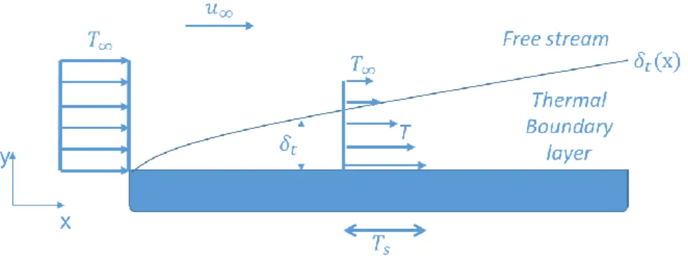
Thermal convection
Thermal convection [52–54] is a process of energy transport through the combined action of conduction, energy storage and mixing. At the molecular level, the thermal exchange by conduction, in fact, is accompanied by a transport of internal energy due to the relative motion of the particles. It is the most important heat exchange mechanism between a solid surface and a fluid (liquid or gas).
A necessary condition for the phenomenon to happen is that the fluid is placed, or can be placed, in relative motion with respect to the other body with which it exchanges heat.
Therefore convection can occur between a solid and a liquid, between a solid and an aeriform, between a liquid and an aeriform, but also between two inescapable liquids. In general it can be said that convection occurs within the fluid in a limited space that begins at the interface between the fluid and the other body and end at a distance that depends on the case under examination, but which is however somewhat reduced.
The transmission of energy by convection, from a surface whose temperature is higher than that of the surrounding fluid, takes place in different stages: first the heat passes by conduction from the surface to the adjacent fluid particles and the energy thus transmitted increases the internal energy and particle temperature.
Since the flow of heat from the surface to the fluid generates variations in the density of the fluid layers closest to it, a movement of the lighter fluid is generated upwards which, when meeting regions of the fluid at lower temperature, mixes with it giving part of the its energy to other particles [55–57]. Therefore there is a flow of both matter and energy, as this is stored in the particles and removed from their motion. Finally, when the heated fluid particles reach a lower temperature region, again the heat is transmitted by conduction from the warmer fluid particles to the colder ones (Fig. 17).