Chapter 2

Chapter 2

Literature Review

2.1 Theory on stirred vessels

Mixing in agitated tanks can be accomplished in different ways. Mechanically agitation, gas sparging and jets are some of the most common. Processing with mechanical mixing occurs either under laminar or turbulent flow, to fulfill the demands of the process operation. A measure of the average turbulence in the system mechanically agitated is obtained by the Reynolds number of the impeller:

μ

ρ 2

Re= LND

Eq 2.1

The condition of complete turbulent flow is achieved for Reynolds numbers higher than 104.

Fluid mixing obtained by means of mechanical agitation has the main purpose of obtaining homogenization in the system. Homogenization is intended for a single or for multiple phases, in terms of the gradient in space of the physical properties such as temperature and for example also of the reduction of gradient of concentration in the system. This is also known as a decrease in the scale of segregation.

Considerable importance in the mixing mechanism is to be assigned to the role of the interaction between the impeller and baffle in the instauration of a turbulent circulation within the vessel.

- Impeller

In the design of stirred tank, the choice of the impeller to be used is of great importance. The flow field generated by the same impeller, varies greatly upon changing characteristics of the configuration, this is due to the complexity of the behavior of the flow.

Different kinds of impellers are used in the industry. A classification of the impeller types can be made dividing them into classes and specific types (see Table 2.1).

Figure 2.1 shows some examples of common axial (A) and radial (R) flow impellers.

Axial flow Propeller, pitched blade turbine, hydrofoils

Radial flow Flat-blade impeller, disk turbine (Rushton),

hollow-blade turbine

High shear Cowles, disk, bar pointed blade impeller

Specialty Retreat curve impeller, sweptback impeller, spring

impeller, glass-lined turbines

Table 2.1: Impeller Classes and Specific types (Edward L.Paul, 2003)

a) b)

c) d) e)

Figure 2.1: a) Chemineer CD-6 (R) b) 4 blade Rushton Turbine (R) c) 4 blade Pitched Turbine (A) d) Marine

impeller (A) e) Hydrofoil (A)

The choice of the right impeller for the system to mix is function of many parameters; the ultimate scope is to obtain a target level of mixing, and doing it in the fastest, cheapest and most elegant way.

- Baffles

Baffles are generally used to break the solid body motion of the flow, increasing the isotropy of the system thus the mixing. Most of the mechanical agitation in vessels is done with the aid of baffling. In particular cases, the use of the baffles is not recommended, for instance, in systems which require frequent cleaning, or where the geometry of the system is enough to guarantee the break up of the solid motion, like in square tanks, or for eccentric agitation (G. Montante et al., 2006).

2.2 Flow Measurements

The flow mapping techniques are intended to determine experimentally the spatial and time coordinates of the instant velocity vector u

(

x,y,z,t

)

. In systems where turbulent conditions are present, the fluctuations of the velocity components increase the difficulty to quantize its values. Flow mapping techniques can be summarized in two main categories, single-point and whole flow field measurement. Both lead to the flow field quantization, but for the single point analysis every velocity component is determined first respect to its variation in time at determined space coordinates and than in post elaboration the flow field is generated recombining these information. For what concerns the whole flow field measurements, in every acquisition, information about the flow field are obtained over a ∂ t.

2.2.1 Single point measurements

The most commonly used techniques to measure single point instant velocities, are briefly discussed in the following lines, and since the scope of this work is not to investigate invasive forms of flow measurements, only the Laser Doppler Anemometry will be discussed as a base to comprehend the differences with the Particle Image Velocimetry, which represents the main technique that allows the measurement of the whole flow field.

- Pitot tube

It is often used to measure the flow in channels, rivers and systems where the relative dimensions of the Pitot tube are small enough to not interfere with the flow structure.

The Pitot tube consists of two concentric tubes, set upstream. The inner tube intercepts the incoming flow, while the outer tube has small openings on the walls to measure the static pressure, the difference in the two pressures, read by a manometer, gives the point flow velocity. A main disadvantage of this system is that is subjected to errors if the probe is not aligned with the flow. This measurement technique is commonly used in turbulence obtained by flow fields generated by free jets (W.R. Quinn, 2005).

- Hot wire Anemometry

Hot wire anemometry (HWA) is another technique that has been used for many years in the study of laminar, transitional and turbulent boundary layer flows and also to measure instantaneous fluid velocities in stirred vessels. The technique depends on the sensing and measurement of the rate of cooling of an electrically-heated fine wire or probe. The wire is usually made of tungsten, platinum, and the diameter is typically 5μm. If only the fluid velocity varies, then the heat loss can be interpreted as a measure of that variable. These anemometers have a high frequency response and thus are well suited to the measurement of unsteady flows. By combining several wires on the same probe, it is possible to measure simultaneously all three components of the velocity vector. The main disadvantage of this technique is that the probe is intrusive and can interfere with the flow. Extensive measurements of turbulence with HWA have been carried out by Stahl Wernersson (1997).

- Laser Doppler Anemometry

This technique is based on the concept of the Doppler shift, this effect can also be observed with sound. When an electromagnetic wave is reflected from a moving object, it changes its frequency proportionally to its frequency shift. By means of this relationship, it is possible to estimate the original velocity of the moving body. This is the basis for LDA. The use of LDA in stirred vessels is associated with the necessity for the fluid in the system to be seeded with particles, which are small enough to behave as much as possible like the fluid in exam. These particles are illuminated at a known frequency of laser light. The scattered laser light is detected by a photomultiplier tube, which transforms the photon energy in electric current and than amplifies the signal. The difference between the incident and scattered laser light frequencies is called the Doppler shift.

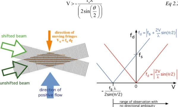
There is however a directional ambiguity, in interpreting the signal, since particles moving in either the forward or the reverse direction will produce identical signals and frequencies. Therefore, in practice, the frequency of one of the beams is slightly shifted, using a Bragg cell: with this frequency shift in one beam relative to the other, the interference fringes appear to move and thus negative and positive velocities can be distinguished. This intersection of the two laser beams produces a well defined interrogation volume. Seeded particles that pass through this volume scatter light and their velocity and direction is defined by:

⎟⎟ ⎠ ⎞ ⎜⎜ ⎝ ⎛ ⎟ ⎠ ⎞ ⎜ ⎝ ⎛ > 2 sin 2 f - V s θ λ Eq 2.2

Figure 2.2: Removing directional ambiguity with frequency shifting. With stationary fringes the detected frequency,

fd, is the same for +V and -V (red curve), i.e. we cannot distinguish direction. To remove this ambiguity we add a frequency shift, fs. Then, as shown by the blue curve, +V and -V produce unique values of fd. The frequency shift is introduced optically by shifting one of the incident light beams by fs. This causes the fringes in the interference pattern to move at Vs = fs df, and shifts the frequency of the scattered light by fs. Directional ambiguity is then removed for V > -fs⎣/ (2sin(⎝/2)).

Because the arrival of each particle is random, the time between velocity estimates is random. So, the velocity is not evenly sampled in time. Before most analyses techniques can be applied to the data, e.g. FFT techniques, the record must be resampled onto an equi-spaced time grid. This, of course, contributes uncertainty to the final analysis. In addition, more samples are generated when the velocity is higher, such that an ensemble-average of the data does not reflect the true time-average. This bias is eliminated by using a time-weighted average, which weights each velocity estimate by the duration of the underlying burst. Assuming the particle concentration is uniform; this provides proportionally higher weight to lower velocity samples, which occur when samples are less frequent.

2.2.2 Whole flow field measurements

- Particle image Velocimetry (PIV)

Particle image Velocimetry was born from the necessity to obtain at the same time the measures of the whole velocity field, rather than a point by point methodology as LDA, described in the previous paragraph. PIV is now a well established technique for the measurement of instantaneous planar velocity fields in macroscopic fluid systems (R. J. Adrian, 1991), and also in micro systems (Santiago et. al., 1998). PIV origins from a measuring technique, the Laser Speckle Velocimetry, applied in the field of the mechanic of solids in the movements of solid bodies subjected to stresses. The PIV is based on the images of tracer particles suspended in the flow. In an ideal system the particles behave exactly like the fluid being prefect flow tracers. A planar laser sheet lights the surface of interest generating micro-pikes due to the surface of the material, analyzing the movement of these pikes is possible to obtain the deformation of the material.

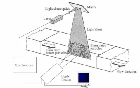
Figure 2.3: PIV system (Raffel et al.., 1998)

In the PIV technique, a laser light sheet illuminates a plane of interest within the flow field, which is seeded with suitable tracer particles, often the same as LDA. Usually a dual head pulsed laser is utilized allowing two laser pulses to be emitted separated by a short user-defined time, t (of order 0.1 ms). Virtually all modern PIV systems utilize digital cameras to image the illuminated plane of interest and then cross-correlation algorithms are used to

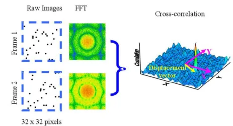
determine the particle displacement in time ∂ t. For each measurement, images A and B (from each laser pulse pair) are separately stored on the camera sensor. The series of double frame images are continuously downloaded to a PC where they are then stored for analysis. Each image frame is discretized into a regular grid of square interrogation cells, which are typically 32 × 32 pixels. Therefore, for calculation purposes, the image consists of a grid of smaller interrogation cells. To ensure a good Signal to noise ratio (SNR) the particles inside each interrogation area, should be around 5 (Raffel et al.., 1998).

The image analysis is based on the correlation between the displacement of the particles in the images, the frequency of acquisition and the actual velocity of the particles in the interrogation area. Based on this, the interrogation window (IW) should be chosen such that the particle displacement within the IW is less than 25% of IW size (Keane and Adrian, 1990).

There are basically two methods to analyse images obtained by the CCD, Auto-correlation and Cross-correlation. In this review, the cross-correlation will be discussed more in detail, since is the technique used in the present work to analyze the images.

For single frame multiple exposure images is used the auto correlation, to get the displacement of a group of particles in an interrogation area. The auto correlation function is similar to the cross correlation.

( )

x I

( ) (

x I x x

)

dx

RII 0 =

∫

+ 0 Eq. 2.3

Where I is the light intensity, x is the position in the image, and xo is the displacement vector between members in an image pair, identified as described below from the Fast Fourier Transform (FFT).

For single-frame single-exposure image, or to be more precise, where two different images are analyzed to obtain the displacement vector the cross correlation is performed:

( )

x y =

_∫∫

I

( ) (

x y J x+x y+y

)

dxdy

R_IJ , , ₀, ₀ Eq. 2.4

Where I is the light intensity of the first image and J is the light intensity of the second image. The spatial coordinates are x and y with respective displacements of xo and y0.

To resolve the above equation, as introduced before, the FFT is used. The cross correlation becomes than, a function of the probability of the displacement in the IW.

Figure 2.4: Schematic representation of the cross – correlation

The two-frame cross-correlation technique is superior to auto correlation methods, having the best signal to noise ratio, no directional ambiguity and the ability to measure zero velocity (Raffle et al., 1998).

For the PIV to give the best result, is necessary that the duration of the light pulse is short enough to capture a neat image of the particles, but is more important to regulate the time ∂ t from two different pulses, in order to have a clear displacement of particles between two images. Time intervals too large increase the possibility that the particles leave the IW. At the same time an interval too short reduces the actual resolution of the measurement.

The cross correlation is then performed for a set of two images, taken at known ∂ t, assigning to every interrogation window, the relative displacement vector. (Keane and Adrian, 1990).

The spatial resolution of this technique depends on the size of the IW in which, the flow field has been divided. Assigning a velocity vector for each interrogation area, a Sub-grid filtering is actually applied; the vector field is determined by locating the centroid of the tallest correlation peak in the cross-correlation plane of images.

2.3 Power number

In stirred tank mixing, one of the most important measurement is the power draw of the system, as many scale-up rules depend heavily on the specific power input. The impeller is characterized by its power number,P_o. Given by:

5 3 D N P P L o ρ = where P=2πNM Eq. 2.5

In other words, it is a dimensionless parameter that measures the power requirements of an impeller. Where is the mechanical power that the impeller transmits to the fluid, the rotational speed , the diameter of the impeller and M the torque on the shaft.

P N

D

In water except for very low rotational speed, the flow is always turbulent, and therefore the tends to be constant over the whole Reynolds region, so for N great enough:

o P Eq. 2.6 5 3 D N P∝

Plotting experimental power data on logarithmic graphs should give a slope of 3.

However, even in turbulent regions, the power number is not completely, constant but is a function of the geometrical parameters of the impeller. For a 45°-pitch, 6-bladed turbine with C/T=0.25 Bujalski et al, (1986) have found that:

(

_/

) (

0.17 _/

)

0.14 78 . 0 − − = D T x D P_o Eq. 2.7

The low impellers, compared with high impellers, operating at same power input P and same geometry, require less torque (

o

P Po

M) and are operated at higher speeds. Lower

means small diameter shafts, seals, gearboxes and so cutting down the costs, (A.W Nienow 1998). o P 5 2 2 1 D N P M = _π oρL Eq. 2.8

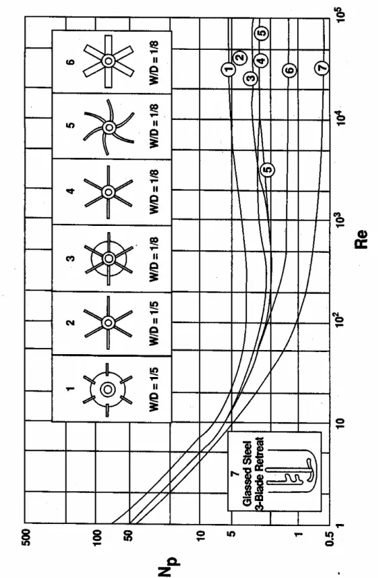
Impellers widely used like the Ruston turbine, are high torque impellers, so they require lower speeds. In Figure 2.5 is reported the difference in the for different types of impellers over a wide range of Reynolds numbers, where W is the impeller width.

o

Figure 2 .5: P o we r numbe r ve rs us impe ller Re ynolds num be r for se ve n di ffer en t impell ers (m odified fr om R u shto n et al., 19 50).

2.4 Flow number

The flow number (Fl) is the measure of the pumping capacity of an impeller. Fl is a dimensionless group, defined as the ratio between the effective non entrained pumped flow, and an impeller characteristic flow rate:

3

D N

Q

Fl = Eq. 2.9

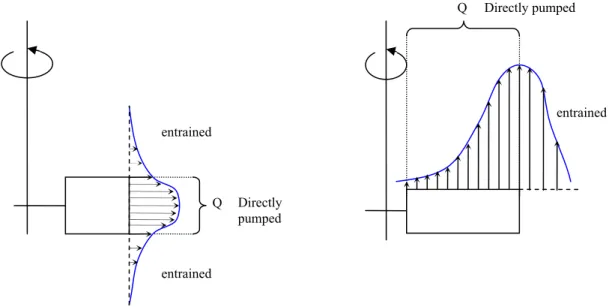
For Q to be calculated, a surface has to be created around the impeller. This surface would be circular for an axial flow impeller and a section of a cylinder wall for a radial flow impeller. The definition of pumping number was first applied to the Rushton turbine:

Directly pumped Q entrained entrained Directly pumped entrained Q

Figure 2.6: Discharge velocity off the tip of a Radial turbine and an Axial turbine.

The actual value of the Fl for most impellers varies from 0.4 of the Chemineer HE3 and 0.8 of the Prochem Maxflo, while for 6-blade 45°-PBT and 6-blade Rushton turbine the flow number is around 0.7 (Weetman and Oldshue, 1998) (Jaworski at al, 1991).

2.5 Turbulent kinetic energy

Turbulence in stirred vessels, as in any other turbulent system, is characterized by random fluctuations of the three components of the velocity observed at a single point. It is usually convenient to describe the turbulence in term of deviation from the time average mean value.

u u

u'_i= _i − Eq. 2.10

Where for a discrete sampling over N intervals:

∑

= N i N u u 1 Eq. 2.11

N is large enough, in order to have a steady u over the complete time sampling interval. To characterize the fluctuating component the root mean square is used:

(

)

2 ~

u u

ui = _i − Eq. 2.12

The root mean square velocity of the fluctuation of one component of the velocity is statistically the same as its standard deviation.

Turbulence is said to be homogeneous when the oscillations of the three components are the same in all point of the system over time. The turbulence that respects this definition is said to be isotopic.

The kinetic energy is the energy associated with the flow, and does not give a measure of the effective mixing. Since the portion of the kinetic energy which actually responsible for the mixing is the one associated with the fluctuations, the turbulent kinetic energy (TKE) is introduced: N w v u k N i i i

∑

_⎟⎟ ⎠ ⎞ ⎜ ⎜ ⎝ ⎛ + + = 1 2 ~ 2 ~ 2 ~ 2 1 Eq. 2.13

Evaluation of TKE implies that information on the three components is available. For some measuring techniques this is not always possible. When only two components can be measured, than the fluctuation velocity of the third component and the turbulent kinetic energy is approximated as:

2 ~ ~ ~ ⎟_⎠ ⎞ ⎜ ⎝ ⎛ ₊ = i i i v u w _⎟⎟ ⎠ ⎞ ⎜ ⎜ ⎝ ⎛ + = ~ 2 ~2 4 3 i i i u v k Eq. 2.14

By doing this is assumed that in a stirred vessel the hypothesis of isotropy is verified in every zone of the vessel.

2.6 Local energy dissipation rates

Accurate estimation of the turbulence dissipation rates is important in order to determine the degree of segregation, droplet and bubble break-down and chemical reaction. Thus the rate of dissipation of scalar concentration fluctuations is a measure of the rate of mixing which is proportional to the rate of viscous dissipation of mechanical energy in turbulent motions (K.V Sharp and R J Adrian, 2001). The resolutions in terms of time space and velocity needed to fully measure the energy dissipation are the Kolmogorov scales.

By assuming that in the viscous sub range, the inertial forces equal the viscous forces, Re=1, it can be written:

4 1 3 ⎟⎟ ⎠ ⎞ ⎜⎜ ⎝ ⎛ = ε υ η

( )

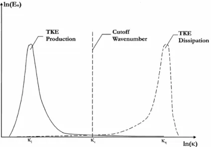
4 1 υε = v 2 1 ⎟ ⎠ ⎞ ⎜ ⎝ ⎛ = ε υ d t Eq.2.15

The hypothesis of equilibrium indicates that the rate of generation of the turbulent kinetic energy in the large-flow depended scales is the same as the rate of dissipation that occurs in the viscous sub-range. In between there is a large region where the energy is not dissipated nor generated, but transferred to lower scales (inertial sub-range). Figure 2.7 illustrates qualitatively the symmetry between energy generated at higher scales with its correspondent dissipation scale, at lower length scales.

In the study of turbulence, various assumptions are made to simplify the approach to the problem. For a model that may resume a turbulent system, based on shear flows transported by a convective flow, can be assumed that eddies do not change as they convect through the system. In other words the turbulent characteristics of the flow remain frozen in time.

This assumption made by Taylor, is known as the Taylor’s frozen turbulence hypothesis:

2 ' 2 2 ' ₁ ⎟⎟ ⎠ ⎞ ⎜⎜ ⎝ ⎛ ∂ ∂ = ⎟⎟ ⎠ ⎞ ⎜⎜ ⎝ ⎛ ∂ ∂ t u U x u _i i i Eq. 2.16

Taylor’s hypothesis is applied specially to point measurements, to solve the problem of measuring the spatial covariance needed to evaluate the turbulent energy dissipation. It is however a strong assumption, which asserts that eddies in time, do not change shape and dimension, or exchange mass. Locking the dynamic features of the turbulent flow. Taylor’s hypothesis is still valid if together with the assumption above, the time needed for the observation of the turbulent eddies is short enough, in this way the eddies do not have time to change significantly during the measure.

In the energy dissipation estimation, the PIV together with others full-field techniques, offers the advantage of obtaining spatial resolved instantaneous velocity in a plane.

2.6.1

Energy dissipation and PIV

The Spatial information provided by the Particle image velocimetry, covers the whole section of the flow field at the same time, so the spatial derivatives can be calculated from the data without the Taylor hypothesis.

The limitation to the PIV measurements is the possibility to resolve the length scales only to some extent. To be able to close on the Kolmogorov scales, usually the viewing area has to be sacrificed. The solution is in increasing the magnification factor, in this way reducing the viewing area, but a trade-off has to be found to identify the correct approach. Finally has to be pointed out that the velocity on which are based the measurements of the physical dimensions like the energy dissipation, are a spatial average of the velocity field in the integration cell, this might as well be considered a filtering effect to the information given by the PIV.

Different models have taken into account the problems listed above, and used different approaches to the evaluation of the energy dissipation.

In the following is presented a short review of the methods applied in this work.

-

Estimating the local energy dissipation from dimensional analysis

Turbulent systems, in which the properties of the turbulence are homogeneous, isotropic and in spectral equilibrium, the turbulence dissipation rate can be expressed as:

l u A 3 ' = ε Eq. 2.17

Wu and Patterson, (1989), proposed the following equation to calculate the energy dissipation directly from the turbulent kinetic energy:

( )

₂ 1/2 2 / 3 3 85 . 0 Λ = k ε Eq. 2.18

Where the is the integral length scale, which represents the correlation distance between to velocity points in the flow field. The degree of correlation tends to decrease increasing the distance on which is calculated.

The integral length scale is defined over one dimension and for one component as (Hinze, 1987):

( )

( ) (

)

( )

2 ' ' x u x u x u R rms x ξ ξ = +

∫

( )

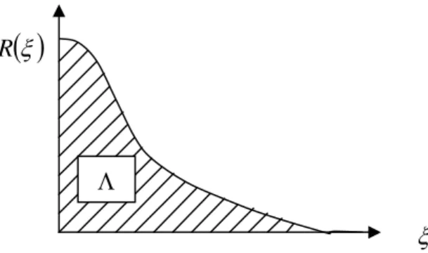
Eq. 2.19 ∞ = Λ 0 ξ ξ d R_x ux

The concept can be easily extended to two dimension analysis (Cheng et al., 1997). In Figure 2.8 is illustrated the graphical meaning of a single dimension autocorrelation described in Eq. 2.19

( )

(

)

12 0 0 , ' , ' ⎟⎟ ⎠ ⎞ ⎜⎜ ⎝ ⎛ + + = Λ

∫

∫

∞ ∞ y x rms y x u d d u y x u y x u ξ ξ ξ ξ Eq. 2.20

From the above equations it is possible to calculate the integral length scales for every component respect to the three dimensions, and for the two dimensional analysis the only one integral length scale for each velocity component can be obtained. The velocity at which the degree of correlation tends to zero and the value that its integral assumes depend only on the conditions around the coordinates. Theξxandξyare the distances at which the degree of

correlation becomes zero.

( )

ξ

R

ξ Λ

Figure 2.8: Graph of qualitative trend of the degree of autocorrelation function of the distance. The integral of

this function is the integral length scale.

This approach has been adopted in previous works (K.C. Lee and M. Yianneskis, 1998) computing the autocorrelation function to the firsts zero crossing.

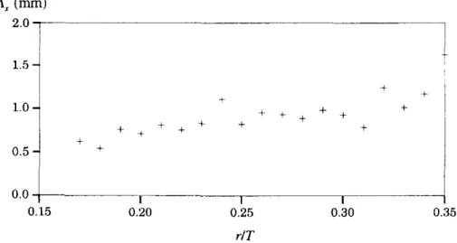
Figure 2.9: Variation of integral length scales with r / T at z/T = 0.33.

(K.C. Lee and M. Yianneskis, 1998)

The length scales inside a stirred vessel depend on the homogeneity of the flow field. This means that in areas where the fluctuation of the velocities are similar and their standard deviation is small, the length scale is going to be higher than in zones where turbulence is less isotopic. Around the impeller typical values of the length scale is of the order of 1 mm, while in the bulk zone is possible to have values which are double.

- Direct measurement of the fluctuating velocity gradient terms in the

definition of energy dissipation

A more rigorous approach to the quantification of local energy dissipation and the effects of the spatial resolution has been widely studied by several researchers, Piirto et al. (2000), Saarenrinne and Piirto (2000); Saarenrinne et al. (2001) and Baldi et al. (2002)). Considering a time averaged turbulence energy dissipation, it can be written (Hinze, 1975):

⎟ ⎟ ⎟ ⎟ ⎟ ⎟ ⎠ ⎞ ⎜ ⎜ ⎜ ⎜ ⎜ ⎜ ⎝ ⎛ ⎟⎟ ⎠ ⎞ ⎜⎜ ⎝ ⎛ ∂ ∂ ∂ ∂ + ∂ ∂ ∂ ∂ + ∂ ∂ ∂ ∂ + ⎟ ⎠ ⎞ ⎜ ⎝ ⎛ ∂ ∂ + ⎟ ⎠ ⎞ ⎜ ⎝ ⎛ ∂ ∂ + ⎟ ⎠ ⎞ ⎜ ⎝ ⎛ ∂ ∂ + ⎟ ⎠ ⎞ ⎜ ⎝ ⎛ ∂ ∂ + ⎟⎟ ⎠ ⎞ ⎜⎜ ⎝ ⎛ ∂ ∂ + ⎟⎟ ⎠ ⎞ ⎜⎜ ⎝ ⎛ ∂ ∂ + ⎟⎟ ⎟ ⎠ ⎞ ⎜⎜ ⎜ ⎝ ⎛ ⎟ ⎠ ⎞ ⎜ ⎝ ⎛ ∂ ∂ + ⎟⎟ ⎠ ⎞ ⎜⎜ ⎝ ⎛ ∂ ∂ + ⎟ ⎠ ⎞ ⎜ ⎝ ⎛ ∂ ∂ = y w z v z u x w x v y u z v z u x w x v y w y u z w y v x u 2 2 2 2 2 2 2 2 2 2 2 υ ε Eq. 2.21

The PIV 2D data are able to give information only about 5 of the components of the above equation. The remaining seven terms are obtained using the local isotropy assumption (Sharp and Adrian, 2001), which gives:

⎟⎟ ⎠ ⎞ ⎜⎜ ⎝ ⎛ ⎟⎟ ⎠ ⎞ ⎜⎜ ⎝ ⎛ ∂ ∂ ∂ ∂ + ⎟ ⎠ ⎞ ⎜ ⎝ ⎛ ∂ ∂ + ⎟⎟ ⎠ ⎞ ⎜⎜ ⎝ ⎛ ∂ ∂ + ⎟⎟ ⎠ ⎞ ⎜⎜ ⎝ ⎛ ∂ ∂ + ⎟ ⎠ ⎞ ⎜ ⎝ ⎛ ∂ ∂ = x v y u x v y u y v x u 2 3 3 2 2 υ ε Eq. 2.22

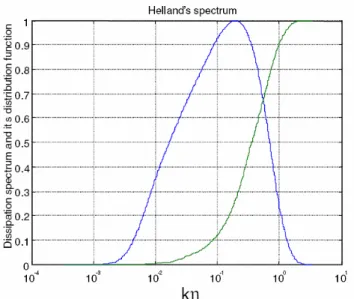
The energy dissipation rate estimated is greatly affected by spatial resolution, where the Kolmogorov length in the bulk region can be ten times greater than in the impeller zone, (Saarenrinne and Piirto, 2000). According to the Figure 2.10, in the bulk zone relatively low spatial resolution and temporal resolution is required, but combined with high velocity measurement accuracy. While in the impeller zone a high spatial and temporal resolution is necessary. In Figure 2.10, the graph of the dissipation rate spectrum, shows the rate of dissipated energy that can be measured, increasing the spatial resolution until Kolmogorov length scale.

Figure 2.10: The dissipation rate spectrum calculated from Helland’s spectrum and its distribution function.

- The large eddy PIV method and Smagorinsky closure model

This method intended by the authors, J. Sheng et al. (2000), to measure the local energy dissipation rates, taking into account that the velocity field obtained by PIV contains all the information for a the spatial derivatives calculation, thus neglecting Taylor’s hypothesis; PIV measurements rarely resolve to the smallest turbulent eddies, and due to the 2-D PIV

limitation of measuring only 2 components, some terms of the dissipation estimation are unavailable and are approximated from the assumption of isotropy of the flow in the vessel.

The method is based on the assumption that the flux of turbulent kinetic energy cascading from the large scales, to the viscous sub range, passing from a broad region where the energy is not generated or dissipated, the inertial sub-range. Thus the flux of turbulent kinetic energy through the inertial sub-range will be equal to the turbulence dissipation rate; it can then be estimated from the PIV. This method does not require the velocity field to be resolved down to the Kolmogorov scale.

This method is based on the idea of the LES simulation applied to the Navier-Stokes equation, in which the terms are filtered by the resolved scale velocity.

The term of the dissipation of the turbulent kinetic energy contains information on the unresolved scales: ε ≈ε_SGS =−2τ_ijSij ⎟⎟ ⎠ ⎞ ⎜ ⎜ ⎝ ⎛ ∂ ∂ + ∂ ∂ = j i i j ij x U x U S 2 1 Eq. 2.23 ij

S is the strain rate tensor computed from the PIV velocity fields.

Therefore the turbulent dissipation rate can be approximately computed by the Reynolds averaged SGS dissipation rate, εSGS. The SGS stress is in the end an approximation of the

kinematic viscosity, that is present in the fully resolved equation, to keep into account the un resolved scales.

The Smagorinsky model or eddy viscosity model is a closure model to evaluateτ : ij

ij ij CS S S 2 2 _Δ − = τ Eq. 2.24

Where the Smagorinsky constant =0.17, S

C Δ is the filter width, and for the PIV is the value of the interrogation window.

Expanding the terms in the previous equation, and neglecting the terms, which influence is very close to zero, the energy dissipation takes the Cartesian form:

2 / 3 2 2 2 2 2 2 ₄ ' ₄ ' ₂ ' ₂ ' ⎟⎟ ⎟ ⎠ ⎞ ⎜⎜ ⎜ ⎝ ⎛ ⎟⎟ ⎠ ⎞ ⎜⎜ ⎝ ⎛ ∂ ∂ + ⎟ ⎠ ⎞ ⎜ ⎝ ⎛ ∂ ∂ + ⎟⎟ ⎠ ⎞ ⎜⎜ ⎝ ⎛ ∂ ∂ + ⎟ ⎠ ⎞ ⎜ ⎝ ⎛ ∂ ∂ Δ = y v x u y v x u CS SGS ε Eq. 2.25

In the above equation the assumption of isotropy in the vessel has substituted the tangential gradients with the PIV resolved.

2.7

Vorticity

Vorticity is the measure of local rotation of the fluid. Mathematically, vorticity is defined as the curl of the velocity vector and can be expressed as:

u × ∇ = ω Eq. 2.26 ⎟ ⎟ ⎟ ⎠ ⎞ ⎜ ⎜ ⎜ ⎝ ⎛ ∂ ∂ ∂ ∂ ∂ ∂ = ⎟ ⎟ ⎟ ⎠ ⎞ ⎜ ⎜ ⎜ ⎝ ⎛ w v u w v u k j i k j i det ω ω ω y u x v k ∂ ∂ − ∂ ∂ = ω

In the study of turbulence in a stirred vessel, vorticity brings information on the size, the strength and the direction of recirculation of the vortexes. Vorticity analysis is therefore used to identify locations of vortices and to calculate vortex statistics. Thus vorticity can be an important tool to study the presence of vortical structures and can be useful to understand how vortices can impact on the turbulence in stirred vessel flows.