NB-IoT synchronization procedure analysis

Master Thesis in

Satellite Communication And Navigation Systems

NB-IoT Synchronization Procedure Analysis

Author: Supervisor:

Riccardo Campana Prof. Ing. Alessandro Vanelli Coralli Co-supervisor: Dr. Matteo Conti Co-supervisor: Dr. Carla Amatetti

Academic Year 2019/2020 Graduation Session III

1.1.1 Stand-Alone Mode of Operation . . . 4

1.1.2 In-Band Mode of Operation . . . 4

1.1.3 Guard-Band Mode of Operation . . . 5

1.2 Physical Layer . . . 5 1.2.1 Frequency Framing . . . 5 1.2.2 Time Framing . . . 6 1.2.3 Downlink Structure . . . 6 1.2.4 Uplink Structure . . . 9 1.3 Protocol Overview . . . 10

1.4 Energy Saving Procedures . . . 11

1.4.1 DRX and eDRX . . . 12

1.4.2 Power Saving Mode (PSM) . . . 14

1.5 Downlink Synchronization . . . 14

1.5.1 NPSS: Time and Frequency Synchronization . . . 15

1.5.2 NSSS: PCID and Initial Frame Synchronization . . . 16

1.6 Random Access Procedure . . . 17

1.6.1 Random Access Preamble . . . 18

1.7 Uplink/Downlink Transmission Procedure . . . 22

1.7.1 Uplink Transmission Procedure . . . 22

1.7.2 Downlink Transmission Procedure . . . 23

2 Satellite NB-IoT Service Provision 25 2.1 System Architecture . . . 26

2.1.1 Transparent Payload . . . 26

2.1.2 Regenerative Payload . . . 27

2.2 Orbits . . . 28

2.2.1 Geostationary Orbit . . . 28

2.2.2 Low Earth Orbit . . . 29

2.2.3 GEO and LEO Scenarios Comparison . . . 30

2.3 Reference Scenario . . . 31

2.4 Doppler . . . 31

2.4.1 Differential Doppler . . . 32

2.4.2 Differential Doppler Assessment . . . 34

2.5 Doppler Mitigation Techniques . . . 35

2.5.1 Frequency Advance . . . 36

2.5.2 CP Based and Map Based Estimation . . . 37

2.5.3 Position Tracking . . . 38

2.5.4 Resource Allocation Strategy . . . 38

2.6 Round Trip Time . . . 39

2.7 Differential Propagation Delay . . . 40

2.8 Delay Implications on NB-IoT Procedures . . . 42

2.8.1 Large RTT Implications on RA Procedures . . . 42

2.8.2 Large RTT Implications on HARQ Procedures . . . 43

2.8.3 DPD Implications on TA Procedure . . . 43

2.8.4 DPD Implications on RA Procedures . . . 44

2.9 DPD Mitigation Techniques . . . 45

2.9.1 Position Tracking . . . 46

2.9.2 New NPRACH Configurations . . . 46

3 Downlink Synchronization Implementation 47 3.1 NPSS Detection Algorithm . . . 47

3.2 NSSS Detection Algorithm . . . 52

3.3 Complexity Evaluation . . . 54

3.3.1 Complexity Of Time Delay Estimation . . . 54

3.3.2 Complexity Of CFO Estimation . . . 54

3.3.3 Complexity Of PCID detection . . . 55

3.3.4 Required UE computational power . . . 55

3.4 Performances . . . 56

CN Core Network

DCI Downlink Control Information DFT Discrete Fourier Transform DPD Differential Propagation Delay DRX Discontinuous Reception

eDRX extended Discontinuous Reception

eNB Evolved Node B, the LTE base station (BS) eNodeB Evolved Node B

FFT Fast Fourier Transform FPO Floating Point Operations GEO Geostationary Earth Orbit

GNSS Global Navigation Satellite System

GW Gateway

HAPS High-Altitude Platform Station HARQ Hybrid Automatic Repeat Request

LEO Low Earth Orbit LoS Line of Sight

LPWAN Low Power Wide Area Networks MAC Medium Access Control

MIB Master Information Block MIB-NB Master Information Block ML Maximum Likelihood

NDI New Data Indicator

NPBCH Narrowband Physical Broadcast Channel

NPDCCH Narrowband Physical Downlink Control Channel NPDSCH Narrowband Physical Downlink Shared Channel NPRACH Narrowband Physical Random Access Channel NPSS Narrowband Primary Synchronization Signal NPUSCH Narrowband Physical Uplink Shared Channel NSSS Narrowband Secondary Synchronization Signal NTN Non Terrestrial Networks

OAI Open Air Interface

OFDMA Orthogonal Frequency-Division Multiple-Access PAPR Peak To Average Power Ratio

PCID Physical Cell Identity

PF Paging Frames

PH Paging Hyperframes PHY Physical

RAR RA Response RF Radio Frequency RFN Radio Frame Number RRC Radio Resource Control RTT Round Trip Time RU Resource Unit Sat Satellite

SatCom Satellite Communications

SC-FDMA Single-Carrier Frequency-Division Multiple-Access SFN System Frame Number

SIB-NB System Information Block SNR Signal to Noise Ratio

TA Timing Advance

TB Transport Block TBS Transport Block Size ToA Time of Arrival

UE User Equipment

1.5 Downlink frame. . . 9

1.6 Uplink resource grid, [3]. . . 10

1.7 Uplink frame, [4]. . . 10

1.8 Overview of NB-IoT protocol procedures. . . 12

1.9 DRX and eDRX current profile, [5]. . . 13

1.10 PSM current profile, [5]. . . 13

1.11 Downlink Synchronization procedure. . . 15

1.12 NPSS and NSSS frame time occurrence, [1]. . . 16

1.13 NPSS detection method. . . 17

1.14 NSSS detection method. . . 18

1.15 Connection Procedure. . . 19

1.16 Coverage classes, [6]. . . 20

1.17 Symbol group and frequency hopping pattern, [1]. . . 20

1.18 preamble detection method. . . 21

1.19 Uplink Transmission Procedure. . . 23

1.20 Downlink Transmission Procedure. . . 23

1.21 Example of uplink transmission scheduling. . . 24

1.22 Example of downlink transmission scheduling. . . 24

2.1 NB-IoT NTN with transparent payload, [7]. . . 27

2.2 NB-IoT NTN with regenerative payload, [7]. . . 28

2.3 Geosynchronous and geostationary orbits. . . 29

2.4 LEO at different inclinations. . . 29 ix

2.5 LEO satellite footprint typology, [7]. . . 30

2.6 Doppler curves of reference UEs, hSAT = 600km, [8]. . . 35

2.7 Doppler curves of reference UEs, hSAT = 1500km, [8]. . . 35

2.8 Doppler shift analysis, [8]. . . 36

2.9 Residual differential Doppler, [9]. . . 37

2.10 System geometry for DPD computation, [7]. . . 42

2.11 Timing Advance analysis, [8]. . . 44

2.12 Cell radius vs Cell center elevation angle, [7]. . . 45

3.1 h and t extraction in one OFDM symbol. . . 50

3.2 Representation of the considered Nf frames. . . 53

3.3 NPSS detection simulator scheme without accumulation. . . 58

3.4 NPSS detection simulator scheme with accumulation of four frames. 58 3.5 NPSS detection simulator scheme without accumulation. . . 59

3.6 Simulation results for Pedelay without accumulation. . . 61

3.7 Simulation results for Pedelay with accumulation of four frames. . . . 61

3.8 Comparison between Pedelay with accumulation and without accumu-lation. . . 62

k

2.4 Reference LEO scenario: hsat = 600km, [8]. . . 40

2.5 Reference LEO scenario: hsat = 1500km, [8]. . . 40

2.6 GEO scenario: hsat = 35786km, [8]. . . 41

2.7 One-way propagation delay and RTT for the considered scenarios, [8]. 41 3.1 Values considered for computational power assessment. . . 56

the management of physical processes, making them more efficient. According to the forecasts of [10], 29 billion connected devices are expected by 2022 of which around 18 billion will be related to IoT. Connected IoT devices include machines, health wearable, meters (water, electric, gas, or parking), connected cars, sensors, point-of-sales terminals, consumer electronics, and so on.

IoT applications may be divided into short-range and wide-area depending on the size of their deployment area. In the former the devices are deployed in a limited area and are connected to the network through the means of unlicensed radio technologies, such as ZigBee, Wi-Fi, and Bluetooth. In the latter, for which the deployment area is theoretically unlimited, the connection to the network mostly relies on cellular networks.

The Third Generation Partnership Project (3GPP), recognizing the importance of IoT, introduced a number of key features to supporting it since Release 13. In par-ticular, since 2017 the so called NB-IoT has been launched, providing progressively improved support for Low Power Wide Area Networks (LPWAN).

While terrestrial technologies will play a key role in the provision of the NB-IoT service, satellite networks can have a complementary role thanks to their very wide coverage area and short service deployment time. Within the aforementioned frame-work, the aim of this thesis is to analyze the feasibility of integrating the NB-IoT technology with satellite communication (SatCom) systems, focusing in particular in the assessment of the downlink synchronization procedure in the NB-IoT SatCom systems. For this reason, this work investigates the issues introduced by the

tion between the NB-IoT terrestrial network and Non Terrestrial Networks (NTN). Furthermore, in order to find possible solutions to harmonize their coexistence, the state of the art of the satellite channel effect mitigation techniques is analyzed. Af-ter that, the implementation of a MATLAB simulator for the cell synchronization procedure is presented, as a first step for the understanding of the whole NB-IoT procedures.

The thesis is divided in four chapters. In the first one, a description of the NB-IoT technology will be provided, thus, the protocol procedures and the Physical layer operation will be analyzed. In the second chapter, the main characteristics of SatCom systems will be presented. Afterwards, the main satellite channel charac-teristics and the implication on the NB-IoT protocol will be investigated. In the third chapter, the NB-IoT synchronization procedures and the implementation of the simulator will be analyzed, then, the simulation results will be presented. The last chapter contains the conclusions and future works.

plexity for user equipment and higher-power consumption. These characteristics are not suitable for IoT applications, which are characterized by low data rates and sporadic transmission of small data payloads. Indeed, NB-IoT is designed as a simplified version of the full-fledged LTE system. This allows to keep the protocol as simple as possible, in order to meet the goals of long device battery lifetime, extended coverage, and low hardware cost. Although NB-IoT is based on existing LTE functionalities, it is a new technology thus not completely backward compatible with the existing 3GPP standard. Despite this, NB-IoT can be deployed in the same eNodeB (eNB) used for LTE, providing pervasive coverage.

The cost of User Equipment (UE) modem is mainly related to the complexity of the Radio Frequency (RF) and baseband sections. For what concerns NB-IoT base-band processing, it has been kept simple by considering a small Transport Block1 (TB) size and by relaxing the processing time requirements compared to LTE. Re-garding RF, all performance goal of NB-IoT can be achieved with single TX-RX antenna, a low accuracy oscillator and an on-chip low-power amplifier [11].

Long device battery lifetime comes along with low power consumption. IoT applications require infrequent transmission of short packets, thus the time in which the UE has no data to transmit or receive, called idle period, is longer than the active time. Since energy consumption during idle mode is much lower with compared to active periods, increasing the time between active periods, allows to significantly reduce energy consumption. In this regard, some techniques increasing the idle

1_{In LTE and NB-IoT the Transport Block is the payload which is passed between the MAC layer}

and Physical Layer [1].

periods duration are adopted in NB-IoT, as described in Section 1.3.

Improved indoor and outdoor coverage has been achieved by trading off data rate for coverage. In fact, repetitions are used to ensure higher system reliability even in challenging locations for coverage, however, this implies a lower data rate. Furthermore, NB-IoT uses a close to constant envelope waveform in the uplink, thus reducing the waste of power due to amplifier inefficiencies [12][1].

1.1

Deployments Options

As previously mentioned, NB-IoT must have the capability of working in parallel with a legacy LTE service as well as being compatible for the deployment in GSM spectrum. Thus, three different deployments options has been designed for NB-IoT: stand-alone, guard-band and in-band.

1.1.1 Stand-Alone Mode of Operation

NB-IoT is in stand-alone mode of operation when it is deployed as a stand-alone carrier, using any available spectrum with bandwidth of at least 180 kHz. This is exceptionally useful for GSM operators who can deploy NB-IoT in a GSM carrier, refarming part of their spectrum. In this type of deployment, NB-IoT has to be compliant with the GSM spectral mask thus its bandwidth becomes 200 KHz. Fur-thermore, a guard band of 100 KHz is recommended between GSM and NB-IoT bands, bringing the total refarmed bandwidth to 400 KHz corresponding to two GSM carriers.

1.1.2 In-Band Mode of Operation

In in-band mode of operation NB-IoT is deployed in the existing LTE networks, using one of the LTE Physical Resource Blocks (PRBs). The PRB is the smallest schedulable unit in most downlink cases and it consists of 12 subcarriers for a total bandwidth of 180 KHz. NB-IoT uses the same modulation and numerology as LTE so it is possible to set a NB-IoT 180 KHz carrier in a LTE PRB without degrading the system performances (without account for PRB number reduction). An example of in-band operation mode is shown in Figure 1.1b.

(a) Guard-band operation. (b) In-band operation.

Figure 1.1: In-band and guard-band deployment options.

1.1.3 Guard-Band Mode of Operation

In guard-band mode of operation NB-IoT is deployed in the guard-band of the existing LTE networks. It relies on the fact that LTE deployment occupies only 90% of its total bandwidth, leaving a 5% available at each side. It is therefore possible to place a NB-IoT carrier in the guard band of LTE, as shown in Figure 1.1a.

1.2

Physical Layer

1.2.1 Frequency Framing

A NB-IoT carrier has a bandwidth of 180 KHz, independently from the deployment mode used. A carrier carrying essential physical signals that allow a device to per-form cell selection is referred to as an anchor carrier. Although only the anchor carrier is strictly required, multicarrier operation is supported. The additional car-riers are named non-anchor carrier and does not carry the physical channels that are required for UE initial cell selection.

In case of in-band or guard- band deployment, the placement of an NB-IoT anchor carrier in frequency is based on a 100 KHz channel raster2, just as for LTE. Contrary to LTE, due to the particular bandwidth of a NB-IoT carrier, an NB-IoT anchor carrier can, however, be located slightly off the 100 kHz channel raster. This fixed positions of carriers in frequency is important since, at start-up, a UE needs to search for anchor carriers in order to select an eNB to camp on. Thus, the UE

2_{In a system that employs a 100 KHz channel raster the carrier center frequency must be an}

can rely on the frequency raster to search for anchor carrier easier.

Furthermore, NB-IoT supports a subcarrier spacing of 15 KHz and 3.75 KHz, implying a carrier subdivision in 12 or 48 subcarriers respectively.

1.2.2 Time Framing

As for the 15 KHz subcarrier spacing, the time unit for the NB-IoT frame is the slot, which is 0.5 ms long. Two slots constitute a subframe and ten subframes constitute a frame, which is 10 ms long (Figure 1.2). While, for the 3.75 KHz subcarrier spacing, the time unit is the slot, which is 2ms long, and five slots constitute a frame of 10 ms, as in Figure 1.3.

Furthermore, 1024 frames constitute a hyperframe and 1024 hyperframes con-stitute a hyperframe cycle which is the highest level of time frame structure [12].

1.2.3 Downlink Structure

As for the downlink, NB-IoT supports only the subcarrier spacing of 15 KHz, which means that in a band of 180 KHz 12 subcarriers can be allocated. In this case the PRB consists of 12 subcarriers in frequency and one subframe in time, as shown in Figure 1.4, [13][12].

Orthogonal Frequency-Division Multiple-Access (OFDMA) is employed in down-link. In order to ensure backward compatibility NB-IoT is designed with the same LTE numerologies. For instance, the same subcarrier spacing, slot, subframe, and frame duration are employed, as well as for OFDM symbol and cyclic prefix dura-tion. The main difference dwells in the modulation and in coding scheme adopted; in fact, QPSK modulation and convolutional coding with 1/3 coding rate are employed, [14].

The messages exchanged on the physical layer between UE and eNB are divided in channels, and each physical channel is in charge of deliver a specific message typology. Furthermore, they are time-multiplexed in a frame, and each channel is scheduled and allocated to an entire subframe and it uses all the 12 subcarriers. A typical structure is depicted in Figure 1.5.

Downlink physical channels are described in the following:

• NPBCH : Narrowband Physical Broadcast Channel is used to deliver the NB-IoT Master Information Block (MIB), which provides essential information for

Figure 1.2: Time framing [1].

Figure 1.4: Downlink resource grid, [2].

the device to operate in the NB-IoT network.

• NPDCCH : Narrowband Physical Downlink Control Channel is used to carry downlink control information. In detail, it delivers uplink grant information, downlink scheduling information and paging information.

• NPDSCH : Narrowband Physical Downlink Shared Channel is used to transmit unicast data.

• NPSS: Narrowband Primary Synchronization Signal is used by the device to achieve synchronization, in both time and frequency, to an NB-IoT cell.

• NSSS: Narrowband Secondary Synchronization Signal is used to detect the Physical Cell Identity (PCID) and acquire more information about the frame structure.

1.2.4 Uplink Structure

As for the uplink, NB-IoT can operate in multi-tone or in single-tone mode. For multi-tone mode, a 15 KHz subcarrier spacing is used while, for single-tone mode, is used a 3.75 KHz subcarrier spacing. Furthermore, sub-PRB transmission is in-troduced in uplink, so the smallest uplink schedulable unit is named Resource Unit (RU) and can have different dimensions. In the basic case, where 12 subcarriers using a spacing of 15 kHz are allocated, the RU corresponds to the downlink PRB seen in Figure 1.4. In the case of sub-PRB scheduling assignments of 6, 3, or 1 subcarrier, the RU is expanded in time to compensate for the diminishing frequency allocation. In single-tone allocation, the subcarrier spacing can be 15 KHz or 3.75 KHz, in the latter the RU spans 32 ms in time. Figure 1.6 shows all the different types of uplink RU, with their bandwidth and corresponding time duration, [12][1]. The uplink is based on Single Carrier Frequency Division Multiple Access (SC-FDMA), also known as Discrete Fourier Transform (DFT) Spread OFDM (DFTS-OFDM). Considering the 15 KHz subcarrier spacing the numerology remains the same as in downlink. For what concerns the modulations, π/4-QPSK or π/2-BPSK are used in conjunction a 1/3 turbo coding. These types of modulation have a very low Peak to Average Power Ratio (PAPR) allowing the transmission with low power backoff. In the extended coverage domain, in which every transmitted watt is important, the power amplifier efficiency introduced by a low PAPR is crucial, [15]. An example of uplink slot format is shown in Figure 1.7. It can be seen that, in case of sub-PRB scheduling, more than one RU can be scheduled in a single time interval.

Uplink physical channels are described in the following:

• NPUSCH : Narrowband Physical Uplink Shared Channel is used to carry up-link user data or control information from higher layers.

Figure 1.6: Uplink resource grid, [3].

• NPRACH : Narrowband Physical Random Access Channel is used by the de-vice to initiate connection and allows the serving base station to estimate the Time of Arrival (ToA) of the received NPRACH signal.

Figure 1.7: Uplink frame, [4].

1.3

Protocol Overview

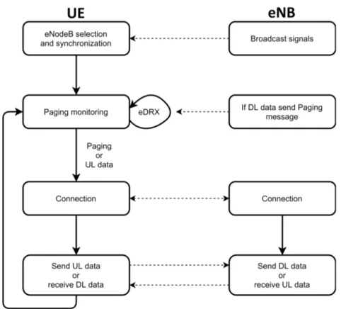
An overview of NB-IoT protocol procedures, divided in four macro areas, is shown in Figure 1.8. The fist two are called Idle mode procedure while the last two are the connected mode procedures.

exchange or for system information updating. Thus, UE periodically listens for possible paging messages from eNB on . The periodicity depends on the eDRX or PSM specific configuration.

• Connection: UE goes in connected mode if it receives the Paging message or if has UL data to transmit. During connection, the UE asks for radio resources and receives other physical layer settings. In this phase we have the random access procedure, when the UE contends the radio resources with the other UEs that need them.

• Data exchange: the eNB sends scheduling information to UE. That radio resources are then used to transmit and receive data and acknowledgements.

1.4

Energy Saving Procedures

NB-IoT user equipment hardware is designed to have a low power consumption in the active state3. However, protracting the active state over time could lead to a quick battery drain. For this reason, 3GPP introduced in NB-IoT some power saving techniques which can extend the battery lifetime.

The user equipment has three main states: active, idle and sleep. In active state the UE absorbs the maximum amount of power due to its transmission and reception activity. In Idle state the UE is on, but the RF section is switched sleep and all the activities are reduced to the minimum. Thus the idle state is characterized by a much lower power consumption. Finally, in the sleep state only a wake up counter is active, thus the power consumption is close to zero.

Therefore, alternating active, idle, and sleep states it is possible to reduce the average power consumption of the UEs. The duty cycle of these different phases is related to the service to deliver. In fact, the longer one is the idle time compared

3

Figure 1.8: Overview of NB-IoT protocol procedures.

to active time, the lower one is the mean power consumption. On the other hand, higher idle time causes an higher latency.

Discontinuous Reception (DRX), extended Discontinuous Reception (eDRX) and Power Saving Mode (PSM) are the main mechanism adopted in NB-IoT for power saving. Three different operation mode are offered in order to fit all possible appli-cation requirements. In Figure 1.9 and Figure 1.10 is depicted the current over time behaviour of DRX, eDRX and PSM.

1.4.1 DRX and eDRX

When the eNB needs to connect with a UE, it sends a PM to the UE in the NPDCCH. The PM can be sent only in predetermined occurrences of NPDCCH called Paging Occasions (PO) and a frame containing a PO is called Paging Frame (PF).

Without using any power saving technique, a UE would have to constantly mon-itor the NPDCCH channel looking for PMs. Although, if DRX is used, the UE monitors the channel with a periodicity multiple of PF. The UE remains active only for the time required to acquire the PF, along with the POs that may be contained

Figure 1.9: DRX and eDRX current profile, [5].

in the subframes of the PF. With DRX the periodicity can not be very long, in fact it can span from 1.28 seconds to 10.24 seconds. This make DRX useful for applications which need lower latency and have relaxed power consumption requirements.

If eDRX is used, the UE monitors the channel with a periodicity multiple of Paging Hyperframes (PH). With eDRX the periodicity can span from 20.48 seconds to 2.9 hours, making it more flexible. If the idle periods are long, the UE can accumulate an imperfect time synchronization with the eNB, due to the possible local oscillators mismatch. For this reason, the UE remains active for a time window longer than a single PF. The period of time in which the UE remains active is called Paging Time Window (PTW), and it can contain different PFs and thus different POs for the UE, [16].

1.4.2 Power Saving Mode (PSM)

For some applications with very relaxed requirements on latency, the mean power consumption can be further reduced by the means of the power saving mode. In PSM the UE is essentially switched off, with only its real time clock running for keeping track of time and scheduled idle mode events like the Tracking Area Update (TAU) timer. With the TAU procedure the UE informs the network about which cell it camps on, and it is triggered when the TAU timer expires. The device exits PSM once it has uplink data to transmit or at the expiration of the TAU timer to transmit the TAU message. After uplink transmission, the device may enter DRX mode for a configured time, to monitor PO, enabling mobile terminated reachability. With PSM some UE idle functions are not available. In addition, at every wake-up the UE has to boot-wake-up from scratch, bringing to an high power consuming phase (Figure 1.10). For this reason, its mean power consumption is lower to the one of eDRX only in case of very long sleep periods, [16].

1.5

Downlink Synchronization

As shown in Figure 1.11 the downlink synchronization procedure can be divided in the following steps:

• UE power on.

NB is transmitted. The SIB-NB is acquired in order to identify the complete SFN, tracking area, and cell identity and to prepare for verification of the cell suitability.

• NPDCCH monitoring to receive PM, ready to start the connection procedure.

Figure 1.11: Downlink Synchronization procedure.

1.5.1 NPSS: Time and Frequency Synchronization

Due to the limited accuracy of the UE oscillator, the device can accumulate a large frequency shift that can be as much as 20 ppm (e.g., 18 kHz in a 900 MHz band).

Therefore, the NPSS needs to be designed to be detectable even with a very large frequency offset. For this reason, NPSS is generated as a hierarchical sequence based on a base sequence p and a binary cover code c. The base sequence p is a frequency-domain Zadoff-Chu (ZC) sequence, [17].

As depicted in Figure 1.12, NPSS is transmitted in subframe number 5 of every frame, thus by detecting the time instant of NPSS the UE can synchronize with the subframe number of the frame. Once the device has acquired time synchronization, it can use the subsequent NPSS signals to estimate the Carrier Frequency Offset (CFO).

Figure 1.12: NPSS and NSSS frame time occurrence, [1].

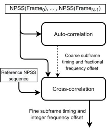
A possible method to extract the time delay and the CFO is shown in Figure 1.13. It is useful to accumulate detection metrics over many NPSS subframes in coverage-limited conditions. For this reason, the first step for NPSS detection is to perform the autocorrelation between some NPSS repetition, to gain a coarse subframe timing and fractional CFO. Exploiting this information, it is possible to gain fine subframe timing and integer frequency offset by performing the cross-correlation between the incoming NPSS signal and the known NPSS sequence, [18].

1.5.2 NSSS: PCID and Initial Frame Synchronization

NB-IoT supports 504 unique physical cell identities and there is a different NPSS se-quence for every PCID. Thus, the cell PCID can be determined by correctly decoding the NSSS. In addition, NSSS is transmitted in subframe 9 in every even-numbered frame and has an 80-ms repetition interval, within which four different NSSS se-quences are transmitted. Thus, by determining which of the four NSSS sese-quences has been received, the UE understands the frame number of the NSSS in the 80-ms time interval. Thus it can reconstruct the three less significant bits of the SFN, [1]. In a cell, all the NSSS transmissions share the same binary scrambling sequence and extended ZC sequence, in fact they are determined by the cell identity k. Within an 80-ms NSSS repetition interval, the four occurrences of NSSS are differentiated

Figure 1.13: NPSS detection method.

by a phase shift.

A straightforward NSSS detection algorithm is to cross-correlate all the NSSS hypotheses with the received NSSS and take the one that have the higher correla-tion, [19]. This allows to identify the PCID and part of the SFN associated to the decoded hypotheses. As for NPSS, in coverage-limited condition, NSSS detection may rely on accumulating detection metrics over multiple NSSS repetition intervals. An illustration of this procedure is shown in Figure 1.14.

1.6

Random Access Procedure

The Random Access (RA) procedure is the procedure a UE initiates to connect to an eNB. It can be initiated by the UE itself, or by an order from the eNB through NPDCCH. The aim of a UE performing RA procedure is to achieve uplink Synchronization, obtain an uplink grant to request the connection to the eNB and finally establish connection. RA procedure relays on the exchange of four messages, Msg1, Msg2, Msg3, and Msg4, as shown in Figure 1.15, [1].

Figure 1.14: NSSS detection method.

Msg1 is the RA Preamble (RAP), it is sent by the UE in NPRACH to initiate the RA procedure and for Time of Arrival (ToA) estimation. If the base station detects a RAP, it sends back a RA Response (RAR) in Msg2. The RAR contains the Timing Advance (TA) parameter, along with the scheduling information used by the UE to transmit the request to connect, known as Msg3. In Msg3 the UE includes its identity as well as scheduling request. Finally, with Msg4, the connection setup message, the eNB resolves any contention that can arise from multiple UE transmitting the same preamble. The connection procedure closes when the UE acknowledges the reception of Msg4, [12].

1.6.1 Random Access Preamble

The network can configure up to three NPRACH resource configurations in a cell, to serve the UEs in different coverage classes which experience different channel con-ditions. Each NPRACH configuration is associated to a different class of preambles and repetition values. In order to estimate its coverage class, the UE measures its downlink received signal power. Afterwards, it transmits the RAP in the NPRACH resources configured for its estimated coverage level.

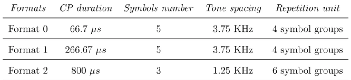
NPRACH preambles use single-tone transmission with frequency hopping. A preamble symbol group consists of a CP and multiple symbols, and a preamble repetition unit consists of multiple symbol groups. The three NPRACH formats available in NB-IoT are described in Table 1.1. As shown, the symbol group for Format 0 and Format 1 consist of a CP plus five single-tone symbols of tone fre-quency n∆fN P RACH, where n is fixed within a symbol group and ∆fN P RACH is the

Figure 1.15: Connection Procedure.

tone spacing of 3.75 KHz. Hence, The resulting NPRACH symbol group consists of a continuous phase sinusoidal waveform of baseband frequency n∆fN P RACH. The

same structure holds for Format 2, but with only three single-tone symbols and ∆fN P RACH = 1.25 KHz.

Formats CP duration Symbols number Tone spacing Repetition unit

Format 0 66.7 µs 5 3.75 KHz 4 symbol groups

Format 1 266.67 µs 5 3.75 KHz 4 symbol groups

Format 2 800 µs 3 1.25 KHz 6 symbol groups

Table 1.1: NPRACH formats characteristics.

NPRACH formats are designed with three different numerologies supporting the different coverage classes they are associated with. For example, format 0 and format

Figure 1.16: Coverage classes, [6].

Figure 1.17: Symbol group and frequency hopping pattern, [1].

1 supports a cell radii up to at least 10 and 40 km, respectively. Whereas format 2 supports a cell radius up to 120 Km.

The hopping pattern design is a prominent feature of NPRACH. It consists of both inner layer fixed size hopping and outer layer pseudo-random hopping. In fact, the frequency hopping starting point is chosen randomly but then the hopping follows a fixed pattern. As depicted in Figure 1.17, there are two levels of subcarrier hopping. The first is used between the first and the second and between the third and the fourth symbol groups. In this case it follows a single-subcarrier hopping with a mirrored behaviour between the first couple and the other. The second level of hopping is a 6-subcarrier hopping and it is used between the second and the third symbol groups.

The rationale behind NPRACH hopping pattern design is twofold. Firstly, it creates a set of NPRACH preambles, within a repetition unit, which are orthogonal

can be estimated decreases increasing the hops size. Whereas, the precision of the estimation increases at lower hops size. In fact, the two levels of frequency hopping are introduced to tackle this existing design tradeoff between ToA estimation range and accuracy when choosing the frequency hopping steps. In fact, single-subcarrier hopping ensures a large enough ToA estimation range to meet NB-IoT target cell sizes, while six-subcarrier and pseudo random hopping improve ToA estimation ac-curacy.

Figure 1.18: preamble detection method.

At eNB side, the preamble has not only a time offset but also a frequency offset. Therefore, the preamble detection algorithm (Figure 1.18) must jointly estimate the phase shifts due to ToA and CFO. The estimate is performed recursively correct-ing the received symbols with hypothesis (T oAH, CF OH) and selecting the one hypothesis that yields the maximum correlation between the received symbols and

the reference preamble. Afterwards, assuming the estimate (T oA∗, CF O∗) has been obtained, the presence of the preamble is determined through the maximum corre-lation value. If the correcorre-lation result exceeds a predetermined threshold[20], the BS declares the presence of the preamble; otherwise, the BS declares that the preamble is not present.

1.7

Uplink/Downlink Transmission Procedure

In this Section, we describe how the procedures for uplink and downlink trans-missions work. The data exchange between UE and eNB is coordinated by the scheduling information provided by the network. When the eNB needs to schedule a device, it sends a Downlink Control Information (DCI) addressed to the device through NPDCCH. The DCI contains information about frequency and time re-source allocation and information needed for the Hybrid Automatic Repeat Request (HARQ) process. Afterwords, the UE uses this information to transmit or receive data in the scheduled radio resources. Uplink and downlink data transmission proce-dure are summarized in Figure 1.19 and Figure 1.20 and are detailed in the following Sections, [21].

1.7.1 Uplink Transmission Procedure

For uplink data transmissions, is required a minimum 8 ms time gap between the last DCI subframe and the first scheduled NPUSCH subframe. This relaxed time scheduling allows the device to decode the DCI and to switch the RF from reception to transmission mode. After being scheduled, the UE transmits its uplink data on the NPUSCH in the scheduled radio resource. Subsequently, the UE has another time gap of at least 3 ms allowing the device to switch from transmission to recep-tion mode and be ready to monitor the next paging occasion in NPDCCH. For what concerns uplink transmission, the HARQ process is implemented trough an implicit acknowledgement. If the New Data Indicator (NDI) is toggled, the device treats it as an acknowledgement of the previous transmission, otherwise the device repeats the last transmission. An example is shown in Figure 1.21.

Figure 1.19: Uplink Transmission Procedure.

Figure 1.20: Downlink Transmission Procedure.

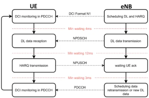
1.7.2 Downlink Transmission Procedure

Differently from the uplink case, in the downlink the minimum time gap between the last DCI subframe and the first scheduled NPDSCH subframe is only 4 ms. In fact, in downlink there is no need for the device to switch from receive to transmit mode between finishing receiving the DCI and starting the NPDSCH reception. After the scheduling information reception, the UE listens the NPDSCH in the scheduled radio resources. Subsequently, the UE must reply with an HARQ message to acknowledge the downlink reception. Thus, in downlink, the scheduler also needs to schedule NPUSCH Format 2 resources for the signalling of HARQ feedback. In this case, a time gap of minimum 12 ms is defined between the ending subframe of scheduled

Figure 1.21: Example of uplink transmission scheduling.

NPDSCH and the starting slot of NPUSCH ensuring sufficient time for the device for decoding information and for switching from reception to transmission. For the same reason, a further time gap of 3 ms is introduced between the HARQ transmission and the subsequent NPDCCH paging occasion. An example is shown in Figure 1.21.

NB-IoT deployment is going to satisfy most of the requirements for a wide range of IoT application in urban areas. On the other hand, there are many IoT scenarios for which terrestrial network deployment is unfeasible or not economically profitable. For these applications, satellite communications (SatCom) have the potential to play an important role. Notably three main areas have been identified in [9]:

• Smart objects for infrastructure or environmental monitoring are often in re-mote locations or they are spread over a wide geographical area (e.g. mid desert pipeline or sea sensors). In these cases, SatCom provides a more cost-effective solution with respect to other terrestrial technologies.

• In the context of critical IoT applications, SatCom can play an important role since reliability is a fundamental requirement.

• Since IoT is characterized by low data rate requirement, satellite operators can find in IoT a profitable way to reuse their low bandwidth satellite infras-tructures, [22].

SatCom solutions have been usually designed for specific tasks and services, with-out cooperation with terrestrial networks. However, in order to serve the plethora of new IoT use cases and services, a new synergy among these two systems must be established. Recognizing its importance, 3GPP is supporting the interoperabil-ity of Non Terrestrial Networks (NTN) and terrestrial communication system since Release 15, [23].

This Chapter aims at analyzing the feasibility of utilization of NB-IoT terrestrial standard on a satellite communication channel. The main issues are investigated, and possible solutions are proposed. In particular, some possible architectures of a SatCom system are presented and a reference scenario for the NB-IoT case is selected. Then, the impact of Doppler shift and long propagation delays on the NB-IoT protocol are investigated.

2.1

System Architecture

In this Section two possible system architectures are presented. Thus, in order to make the discussion clear, the most important architecture components are pre-sented: i) the Core Network (CN) is the central part of the overall mobile network and is responsible to manage some network level procedures of the protocol; ii) the Gateway (GW) is the on-ground transceiver that connects the satellite to the core network; iii) the Satellite (Sat) is the spacecraft responsible to connect the GW with the UEs.

In the direct access scenarios shown in Figure 2.1 and 2.2 the user link (between Sat and UEs) directly involves the satellite and the on-ground UEs by means of the NB-IoT air interface. This air interface is specifically designed for terrestrial systems and, thus, it is fundamental to assess the impact of the satellite channel impairments on both Physical (PHY) and Medium Access Control (MAC) layer procedures. With respect to the feeder link (between Sat and GW), the air interface to be implemented depends on the type of satellite payload1_{. Indeed, in the next}

two Sections transparent and regenerative payloads will be presented.

2.1.1 Transparent Payload

As for the transparent payload satellite, the system eNB is conceptually located at the GW providing the connection towards the CN and the public data network. More specifically, the signals received by the satellite user beams are amplified, filtered, and translated infrequency; then, the signals are retransmitted toward the terrestrial gateway through the feeder link on dedicated frequency band. An opposite path is

1_{The payload is the part of the satellite spacecraft dedicated to telecommunication purposes.}

Considering the transparent payload, it includes the antenna, low and high power amplifiers, filters and frequency converters. Furthermore, the regenerative payload includes also the demodulator, the modulator and computing capability in order to perform some protocol functions also at the satellite.

Figure 2.1: NB-IoT NTN with transparent payload, [7].

followed by the signals flowing from the gateway to the UE. The described system architecture is shown in Figure 2.1. In this architecture, the feeder link air interface is again provided by the terrestrial NB-IoT, thus, the impact of the different satellite channel impairments has to be assessed also in this case.

2.1.2 Regenerative Payload

As for the regenerative payload satellite, the system eNB is implemented on the satellite, while the GW simply provides the connection towards the CN and public data network. In this case, all the eNB functions are performed in the satellite, thus, only the user link must be implemented using the NB-IoT air interface. On the contrary, the feeder link can be implemented relying on any suitable air interface. This architecture has higher cost compared to the transparent payload since it is clearly more complex. However, it significantly reduce the satellite channel effects on the NB-IoT protocol. In fact, the physical and MAC procedures can be directly terminated on the on-board eNB instead of requiring to go down to the GW, thus the propagation delays are significantly reduced.

Figure 2.2: NB-IoT NTN with regenerative payload, [7].

2.2

Orbits

In this Section the different types of satellite orbits and constellations are presented. 3GPP has focused on Geostationary Earth Orbit (GEO) and Low Earth Orbit (LEO) constellations for the deployment of NB-IoT. A third deployment possibility is the High-Altitude Platform Station (HAPS). In this context, it consists of an aircraft, e.g. balloons or airplanes, that operates in the atmosphere at high altitudes for extended periods of time, in order to provide the NB-IoT service. However, the channel impairments introduced by the HAPS deployment are far less severe com-pared to GEO and LEO. Therefore, only GEO and LEO orbits are tackled in the following Sections.

2.2.1 Geostationary Orbit

A geosynchronous orbit (Figure 2.3) is characterized by an orbital period of 24 hours, meaning that the satellite movement along its orbit is synchronous with the Earth’s rotation. When a geosynchronous satellite is placed on the equatorial plane, at altitude of 35.787 Km, the orbit is said geostationary. In this case, an observer from earth sees the geostationary satellite in a fixed position in the sky. This equatorial

Figure 2.3: Geosynchronous and geostationary orbits.

geosynchronous orbit is very crowded due to its unique characteristics. Thus, in order to avoid interference between adjacent GEO satellites, each satellite is assigned a well delimited orbital slot, which corresponds to a distinct longitudinal position.

2.2.2 Low Earth Orbit

Figure 2.4: LEO at different inclinations.

LEO satellites altitudes range between 500 and 2000 km, involving orbital periods between 94 and 127 minutes, [24]. The orbit inclination is the angle of the orbit in relation to Earth’s equator. A satellite that orbits directly above the equator has zero inclination. If a satellite orbits from the geographic north pole to the south pole, its inclination is 90 degrees. LEO satellites can be deployed at any inclination angle as seen in Figure 2.4. However, the deployment of a satellite at inclination value of either 28.5 degrees or 57 degrees can be easier, due to typical launch locations, [25].

LEO orbits are usually exploited for earth observation and communication satel-lites. For what concerns the satellite footprint, two types of deployment have been considered by 3GPP: Earth-moving beams and Earth-fixed beams. In the former, as depicted in Figure 2.5a, the satellite beams follow the satellite movement along the orbit, implying a coverage of a fixed point on Earth for just a few seconds. In the latter, as depicted in Figure 2.5b, the satellite realizes spotbeams that remain fixed on Earth2.

(a) Earth-moving cells. (b) Earth-fixed cells.

Figure 2.5: LEO satellite footprint typology, [7].

2.2.3 GEO and LEO Scenarios Comparison

Making use of GEO it is possible to obtain a full earth coverage, polar region ex-cluded, deploying only three satellites and gateways. By contrast, LEO presents a totally different scenario. In this case, in order to provide real-time global Earth coverage, the number of satellites and gateways required is much larger, and de-pends on the chosen orbit and the surface covered by the satellite antenna. In order to decrease the deployment and operational costs of the system one can reduce the number of LEO satellites selecting an inclined orbit. This ensures good coverage of the Earth after a given number of spacecraft revolutions; thus, it is a viable solution only when the message delivery latency is not an issue. Moreover, the number of terrestrial gateways can be reduced to one using a regenerative payload (Figure 2.2), hence deploying all eNB functionalities on the satellite.

LEO is characterized by high Doppler shift with compared to GEO. However, LEO constellations provide reduced round trip time compared to GEO, which, as discussed in section 2.5, is of relevance in NB-IoT protocol. Moreover, LEO is

2_{The satellite can steer the spotbeams by tilting its antenna or by the means of attitude}

To analyze the implementation feasibility of the NB-IoT terrestrial standard in a satellite channel, a reference scenario must be defined.

As aforementioned, not only, satellite links introduce very large propagation delays compared to terrestrial links, but also, GEO introduces larger delay than LEO. Since NB-IoT terrestrial technology is sensitive to high propagation delays, in the following we focus on LEO satellites, considering an altitude between hsat =

600km and hsat = 1500km. For what concerns the operational frequency, it is

constraint by the NB-IoT standard in the S-Band, i.e., 2170-2200 MHz downlink and 1980-2010 MHz uplink.

In terms of system architecture, the reference scenario is defined by the following assumptions: i) the on-ground UEs are directly connected to the satellite; ii) the satellite is assumed to be transparent and to provide backhaul connection between the GW and the on-ground UEs; iii) the satellite provides coverage through Earth-moving beams; iv) the GW is connected to the satellite through an ideal feeder link, providing access to the terrestrial CN. The defined reference scenario is shown in Figure 2.1.

In the next Sections the main satellite channel impairments introduced by this reference scenario are analyzed.

2.4

Doppler

The Doppler shift consists in the offset in the carrier frequency due to the relative motion between the transmitter and the receiver. In satellite communications, the Doppler shift can be caused by the user terminals’ mobility on ground, but it is mainly due to the satellite movement on its orbit.

A closed-form expression for the Doppler shift as a function of the satellite orbital velocity and the elevation angle θ has been defined in [26]:

fd(t) =

fc· ωsat· RE· cos(θU E(t))

where ωsat = pGME/(RE + hSAT)3 is the satellite orbital velocity, RE is the

Earth radius, G = 6.67 · 1011N m2/kg2 the Gravitational constant, and ME = 5.98 ·

1024 Kg the Earth mass.

When considering GEO systems serving fixed on-ground UEs, the relative veloc-ity between satellite and UEs is negligible, thus the Doppler shift can be assumed to be negligible. Nevertheless, for what concerns the LEO satellites considered in the reference scenario, the orbital speed is high Thus, the relative velocity between satellite and UEs os often considerable, leading to a Doppler shift which can be significantly higher with compared to Doppler expected in terrestrial systems.

2.4.1 Differential Doppler

In the reference scenario, the Doppler experienced by the i-th user in the DL channel and, viceversa, on the satellite with respect to the i-th user in the UL channel consists of two contributions. It can indeed be described as f di = f dcommon+ ∆f di, where

f dcommon is the common part of the Doppler experienced by every user in the same

footprint while ∆f di, the differential part, depends on the relative positions of users

in the footprint, [8].

The main contributor towards the differential Doppler shift is the change of position along the direction of the satellite movement (x axis), whereas for the per-pendicular one (y axes) differential Doppler is negligible. The maximum differential Doppler shift given the cell radius x can be calculated as derived in [27]:

∆f_dM AX =     fc· ωsat· RE c · (cos(θU E1(t)) − cos(θU E2(t)))     (2.2)

Considering the DL user link (from Sat to UE), the differential Doppler is not an issue since each UE must compensate its own experienced Doppler f di. Indeed,

each UE under the same Doppler condition will receive the whole bandwidth of 180 kHz, with negligible effects on the single subcarriers. On the other hand, In the UL user link (from UE to Sat), each UE generates its own SC-FDMA signal, thus the differential Doppler must be compensated such that the frame structure seen by the satellite does not contain overlapping information among subcarriers, [8]. Furthermore, the feeder link (from eNB to Sat and viceversa) can be considered ideal,

the users positions and the differential Doppler experienced.

The received baseband signal at the eNB due to the differential Doppler between UEs is given by : yR= N X k=1 xU Eke −j2πf_dk(t)t_{= e}−j2πf_d1(t)t N X k=1 xU Eke −j2π∆f_dk(t)t _(2.3)

where fdk(t) = fd1(t) + ∆fdk(t) and fd1 is the Doppler of one user in the cell

taken as a reference. The nomenclature adopted in the mathematical formulation can be found in Table 2.1, [8].

Definition Symbol

Number of nUE in the cell N

RX baseband signal nU EK → eN B YR

TX baseband signal nU EK → eN B xU Ek

nUEs carr. freq. off. (coomon) w.r.t. eNB fko

Differential Frequency Offset pf nUEs f∆k

Freq. off. added by nU Ek loc. osc. fk= fko+ f∆k

Doppler added at t for k-th user (Sat → nU E) fdk(t)

Doppler added at t + τ for k-th user (nU E → Sat) fdk(t + τ )

Table 2.1: Nomenclature for Doppler analyzes.

Looking at this expression, the common part (e−j2πfd1(t)t_{) can be easily}

Doppler amongst users must be pre-compensated at each UE to avoid dangerous degradation.

As discussed in 3GPP specifications [28] and [29] about mobile UEs, LTE phys-ical layer is specifphys-ically designed to tolerate a Doppler up to 950 Hz, considering a carrier frequency of 2 GHz and a maximum relative speed at 500 km/h. Therefore, since f dcommon can be compensated at the eNB, it is possible to assume that for a

subcarrier spacing of 15 kHz a value of ∆f di up to ≈ 950 Hz could be tolerated. Proportionally, for a subcarrier spacing of 3.75 kHz the value of ∆f di should be lower than ≈ 240 Hz [9], to fulfill the constraints on Doppler for NB-IoT.

2.4.2 Differential Doppler Assessment

The purpose of this paragraph is to quantify the differential Doppler in worst-case conditions and compare the results with the constraint given by NB-IoT. Simulations have been performed in [8] considering the parameters in Table 2.2. Figures 2.6 and 2.7 show the Doppler behaviour over time for two UEs placed at different distances in the coverage area. The differential Doppler, as seen by the satellite antenna at each timing instant, is the difference between the curve of the considered distance and the reference curve, and it is highlighted in Figure 2.8. It can be noticed that the worst-case differential Doppler increases at higher distances and decreases at higher orbits.

Parameter Value

Carrier Frequency 2.2 GHz

Satellite altitude range 600-1500 km

Elevation angle 90◦

Minimum elevation angle 10◦

Reference UEs reciprocal distance 40-200 km Table 2.2: Simulation Parameters.

It is worth to notice that the differential Doppler values from simulation in Figure 2.8 are compliant with LTE Doppler constraint only for small maximum distances and high orbits. Therefore, the only way to keep the differential Doppler shift under LTE Doppler constraints, without modifying the existing standard, is

Figure 2.6: Doppler curves of reference UEs, hSAT = 600km, [8].

Figure 2.7: Doppler curves of reference UEs, hSAT = 1500km, [8].

to reduce the cell size. As mentioned in the last Section, the differential Doppler depends only on the UE distance on the x-axes, therefore it can be worth to consider ellipsoid cells with the mayor axis in the y direction.

The limitations on the cell radius and orbits can become very stringent without modifying the existing standard. Thus, the design of some technique to reduce the Doppler down to the limit reported in the previous section can be beneficial.

2.5

Doppler Mitigation Techniques

To mitigate the Doppler effect using a pre-compensation procedure each UE must know the instantaneous Doppler that he generates at the satellite antenna. The

Figure 2.8: Doppler shift analysis, [8].

carrier error is generated by the channel and it is not a straightforward information to obtain, thus some estimation technique should be adopted. In the following Sections, a non exhaustive set of estimation techniques, selected after a state of the art analysis, is proposed.

2.5.1 Frequency Advance

A useful technique to be considered for Doppler mitigation is the so called frequency advance. It allows to estimate the frequency offset in the forward link and then reuse it to reduce frequency offset in the reverse link. In general, this technique is not designed for differential Doppler mitigation, but it can be adapted to this scope. Indeed, in [9] is proposed a method based on the estimation of the Doppler experienced in UL based on the DL channel.

It is demonstrated that if the UL transmission occurs within a sufficiently small time interval (τk) after the offset has been estimated on the DL signal, the Doppler

can be assumed almost constant. In this case, using the offset estimated on the DL channel with opposite sign in the UL transmission, the undesired differential Doppler can be mitigated.

In order to evaluate the maximum value for τk, it is necessary to compute the τk

value that corresponds to a residual differential Doppler compliant with the NB-IoT maximum Doppler requirement. The maximum allowed values for τk derived in [9]

are reported in Table 2.3. The results of the simulation are reported for satellite altitude value ranging from 300 to 1200 km and considering the worst case scenario. The residual differential Doppler over time (for τk = 1337ms) is depicted in Figure

Figure 2.9: Residual differential Doppler, [9].

2.9 and it can be seen that the Doppler requirements are respected. Finally, in [9] the typical values of τk for an hypothetical system are assessed, concluding that in

case of 100% gateway availability τk will never exceed its maximum values.

hSAT τM AX ∆fsc = 15 kHz τM AX ∆fsc = 3.75 kHz

300 km 1337 ms 303 ms

800 km 9378 ms 2356 ms

1200 km 22511 ms 5686 ms

Table 2.3: Maximum values for τk, [9].

2.5.2 CP Based and Map Based Estimation

In this Section, two methods for the Doppler estimation in OFDM-based waveforms are reported, since they can be useful for the estimation of the Doppler experienced by each user.

In the first method, the Doppler is estimated by using a cyclic prefix based algo-rithm in [30]. This method is shown to have good performance in AWGN channels while it suffers in multipath channels, [31]. In addition, the maximum Doppler shift

that can be estimated by this CP-based algorithm is half of the subcarrier spacing. In the second method, a MAP Doppler estimator presented in [32], a two step approach is used. In the first step, the algorithm performs a first estimation relying on the cyclic prefix. In the second step, the estimation is refined considering the predictable characterization of the Doppler given by the known circular orbit of a LEO satellite. An interesting advantage of the technique is the possibility to work with mobile terminals up to a speed of 500 km/h, while keeping a low MSE for the Doppler shift estimation (≈ 10−5dB).

2.5.3 Position Tracking

As analyzed in [24], a UE may use its Global Navigation Satellite System (GNSS) location information in combination with satellite ephemeris data to compensate for Doppler effects to a high extent. A residual Doppler shift can occur in case of an error in the estimation of the relative position between the UE and the satellite. The difference between the compensated and the actual Doppler shift can be computed from geometrical considerations and in order to keep the residual Doppler shift below 950 Hz, it is possible to conclude that the position error must be smaller than 4 km, [26].

Even though GNSS integration is compatible with the current NB-IoT devices, a GNSS receiver can drain part of the battery life of the UE, as well as increase the device cost. A straightforward solution for this high power consumption, would be to periodically disable the GNSS exploiting the latest position information for the differential Doppler estimation. This method decreases the energy consumption, but it impacts on the accuracy of the estimation.

Nevertheless, while this solution based on the UEs position can be applied on the existing NB-IoT devices, an additional algorithm, like the aforementioned ones, would result in an additional core to be included in the standard chip.

2.5.4 Resource Allocation Strategy

In [33], in order to limit the differential Doppler shift up to a level supported by the standard, a resource allocation strategy is proposed. Basically, the method consists in splitting the coverage area in smaller regions such that the UEs in each region experience a maximum reciprocal differential Doppler below the allowed threshold. Then, the eNB allows the connection of UEs one region at a time. As a result, the eNB schedules in adjacent time slots only the UEs which have low reciprocal

compared to those of terrestrial networks, resulting in possible problem for some protocol procedures. Depending on the type of procedure analyzed, the one-way propagation delay or the Round Trip Time (RTT) shall be considered. Since the signal processing time in a SatCom context can be assumed negligible with respect to the propagation delay, the RTT can be approximated by twice the propagation delay between the transmitter and the receiver. As stated in [8], in the general case in which the transmitter and the receiver are not perfectly aligned,i.e., they have different elevation angles, the overall RTT can be computed as:

RT T ≈ 2Towp = 2

dGW −Sat(θGW) + dSat−U E(θU E)

c (2.4)

Where Towp is the one-way propagation delay, dGW −Sat is the gateway-satellite

distance as a function of the gateway elevation angle θGW, dSat−U E is the

satellite-UE distance as a function of the satellite-UE elevation angle θU E, and c the speed of light.

An example of RTT computation has been presented in [8]. The following pes-simistic scenario has been considered for the computation. The system GW is as-sumed to be at θGW = 5◦, elevation angle, while the minimum elevation angle for

the UEs is assumed to be θU E = 10◦. The results for the single path distances

and the involved delays, considering both the minimum and the maximum satellite altitude of the reference scenario are listed in Table 2.4 and Table 2.5 respectively. Additionally, the results for the GEO scenario are listed in Table 2.6 for compari-son. Finally, the one-way propagation delay and the RTT can be obtained, they are shown in Table 2.7.

While in the GEO scenario the propagation delay might be an issue for all procedures, with respect to our reference scenario a case-by-case evaluation of the

Elevation angle Path Distance [km] Delay [ms]

UE: θU E = 10◦ Sat-UE 1932.25 ≈ 6.44

GW: θGW = 5◦ Sat-GW 2329.03 ≈ 7.76

Table 2.4: Reference LEO scenario: hsat = 600km, [8].

Elevation angle Path Distance [km] Delay [ms]

UE: θU E = 10◦ Sat-UE 3647.55 ≈ 12.16

GW: θGW = 5◦ Sat-GW 4101.72 ≈ 13.67

Table 2.5: Reference LEO scenario: hsat = 1500km, [8].

delay impact is needed.

For example, even if the latency constraints in NB-IoT are relaxed, some protocol timers must be taken into account into the investigation. In particular, some timer in the Random Access procedure and Radio Resource Control (RRC) procedures can be incompatible with satellite RTT delays. Furthermore, a long RTT has an impact on the UE battery life because it implies longer wake up period for UEs in order to perform RA procedures and data transmission.

2.7

Differential Propagation Delay

In this Section, the Differential Propagation Delay (DPD) is introduced. If the UEs are located in different positions on the cell, they have a different slant range. Furthermore, this difference in the propagation distance between the UEs yields a difference in the propagation delay. The DPD can be described as f deli =

f delcommon+ ∆f deli, where f delcommonis the common part of the delay experienced

by every user in the same footprint while ∆f deli, the differential part, depends on

the relative positions of users in the footprint. The common part is compensated by the UE in the downlink synchronization procedure, when it acquires time synchro-nization with the eNB.

Some NB-IoT procedures require that the signals from different UEs arrive at the eNB within a maximum DPD, which can be adapted based on the coverage area. In particular, the maximum cell radius is strictly connected with the timing constraints of TA and RA procedures. In terrestrial systems there is maximum DPD when a

Scenario One-way [ms] RTT [ms]

GEO ≈ 272.37 ≈ 544.75

Ref. GEO at hsat = 600km ≈ 14.2 ≈ 28.4

Ref. GEO at hsat = 1500km ≈ 25.83 ≈ 51.66

Table 2.7: One-way propagation delay and RTT for the considered scenarios, [8].

UE is located close to the eNB and the other at the cell edge, and it is often not a limiting factor. On the other hand, considering SatCom systems with significantly longer RTT with respect to terrestrial communications, the DPD becomes one of the critical aspects and the cell dimension must be dimensioned according to it.

In our reference scenario, on the user link (UEs ↔ satellite) each UE trans-mission has a different propagation paths and, thus, introduce a differential delay. Differently, the feeder link (satellite ↔ eNB) is common to all UEs and, thus, it does not introduce any DPD in the signal propagation. For this reason, only the user link is considered in the following.

To compute the maximum DPD of a specific cell with radius x, the worst-case scenario in which two UEs are located at the cell edge on opposite location is con-sidered (as depicted in Figure 2.10), and the differential slant range among those two UEs is computed. From [7]:

∆D = Dmax(αmin) − Dmin(αmax) (2.5)

∆D = ( q

R2

Esen(αmin)2+ h2s+ 2REhs− REsen(αmin))− (2.6)

−( q

Figure 2.10: System geometry for DPD computation, [7].

Then, the maximum DPD for the considered cell is computed as ∆Tpd= ∆D_c .

2.8

Delay Implications on NB-IoT Procedures

In this Section, the implications of delay on the NB-IoT procedures is analyzed. In Sections 2.8.1 and 2.8.2 the focus is on the possible issues caused by the large RTT on RA and HARQ procedures. Afterwords, in Sections 2.8.3 and 2.8.4 the implications of the DPD on TA and RA procedures are presented.

2.8.1 Large RTT Implications on RA Procedures

When the UEs send the preamble in Message 1 to starting the RA procedure, they wait for a limited time (RAR time window) to receive back the RAR message from the serving eNB. The choice of the RAR time window is performed by the UE depending on the SNR estimation on the downlink signal, and on the number of repetitions used to transmit the NPRACH preamble. It is worth noting that the

SatCom context, is extended up to 10.24 s, [28]. In summary, the extension of RAR time windows, between message 1 and 2, and of the contention resolution timer, between message 3 and 4 up to 10.24 s, allow to cope with the characteristic RTT of a SatCom system and, thus, no procedure modifications are needed.

2.8.2 Large RTT Implications on HARQ Procedures

The high RTT of SatCom has no implications on the HARQ procedures feasibility in general. Either in the case of data exchange HARQ or Random Access HARQ. Nevertheless, while in the former the RTT arises a problem of increased power consumption, in the latter it can have implications also on the capacity of the cell. In fact, in RA procedure are used two HARQ procedures (in message 3 and in message 4) so the overall procedure time is significantly increased in SatCom implying a degradation of the RA success probability, [7].

2.8.3 DPD Implications on TA Procedure

As discussed in the previous Chapter about NB-IoT, the TA computation is per-formed from the UE assisted by the eNB and follow the same steps as legacy LTE. The eNB measures the ToA of the RA preamble and sends this information back to the UE with the timing advance command. Upon reception of the command, the UE shall adjust the uplink transmission timing for NPUSCH accordingly to it. In [8] is illustrated that for NB-IoT it is possible to compensate a DPD in the uplink transmission, up to a maximum of 0.6667 ms, which is the same value supported for maximum TA in legacy LTE. This means that, if the DPD of the worst case scenario is lower than 0.6667 ms, no modifications to the TA procedure are needed.

In Figure 2.11 are depicted the results of the simulation performed in [8] using the parameters of Table 2.2. Each line in the graph is associated to a scenario with different cell diameter and orbit altitude, and the zero in the time axis corresponds to the maximum elevation angle of 90◦. It can be seen that for each scenario there

Figure 2.11: Timing Advance analysis, [8].

is a time window for which the maximum DPD is lower than the maximum TA allowed by the protocol. Thus, no modifications to the standard are required if the transmission is performed inside these time windows.

It is worth highlighting that the grater is the cell diameter, the shorter is the allowed transmission time period, keeping the orbit altitude as a constant. Although this do not prevent the protocol to work, it actually imposes a limitation to the maximum cell dimension.

2.8.4 DPD Implications on RA Procedures

Before initiating the RA procedure, the UEs are not yet synchronized in time, since TA procedure is performed later. Therefore, due to differential delay, when many UEs attempt to connect with the eNB through message 1 transmission, their pream-bles will be misaligned in time. Furthermore, the protocol can work only if the time misalignment does not exceed the preamble CP length.

The requirement on the maximum preamble misalignment can be formalized as:

∆D < c · Tcp/2 (2.7)

It is known from (2.5) that ∆D depends on the slant range of the closest and the farthest UEs to the satellite. Dmax is associated with the elevation angle αmin that

is set to 10◦ for this computation. On the other hand, Dmin is associated with the

In Figure 2.12 is plotted the cell radius as a function of the cell center elevation angle αcen, for the three existing NPRACH configurations. In the graph are

empha-sized the points where the αmaxreaches 90 degrees, hence the minimum slant range

will coincide with the satellite altitude Dmin = hs. It is worth noticing that the

computations are referred to an orbit altitude of 600 Km, but since DPD decreases with the orbit altitude, the higher the orbit the larger the cell radius would be.

Figure 2.12: Cell radius vs Cell center elevation angle, [7].

2.9

DPD Mitigation Techniques

The analysis presented in the last Section has highlighted the issues caused by DPD on RA and TA procedures. Therefore, in this Section, two DPD mitigation

tech-niques are presented.

2.9.1 Position Tracking

As discussed in Section 2.5.3 for Doppler mitigation, a UE may use its geographical location in combination with satellite ephemeris data to estimate the service link propagation delay. Thus, the transmission of the random access preamble can be time synchronized by compensating for the estimated delay.

Typically, the RA preamble reception is a sensitive operation because the pream-ble is transmitted by the UEs without any knowledge of their specific propagation delay. Only after the transmission of the TA command the UE can have a more precise time synchronization. By contrast, making use of the GNSS location the UE can be time synchronized already from the first transmission.

2.9.2 New NPRACH Configurations

GNSS is not always a viable solution due to its high power consumption. In this case the only way to increase the cells dimension, as discussed in [7] is to introduce new preambles with longer CP lengths. This can give more degrees of freedom to the eNB in selecting the size of the cell, adapting it to the specific Earth region requirements.

NB-IoT rely on the estimate of the received power to select the appropriate NPRACH configuration. However, to fully exploit this additional NPRACH config-urations, the eNB should be able to notify the UE with the information based on its orbit. In fact, this would greatly help the UEs to take proper decisions regarding the NPRACH configuration.

As proposed in [7], the orbit information fields may be included in the DCI along with other fields to continuously update the UEs with new TA values. Since the continuous TA estimation must be done at the eNB using the ToA of signals coming from different UEs, it can not be very precise. Nevertheless, in this way the UEs will be able to remain time-synchronized and avoid multiple RA procedures.