Chapter 4 – PANTHERMIX and MCNP5 CODES
4.1 Introduction
In this Chapter we are going to briefly describe PANTHERMIX [4-1] and MCNP5© codes [4-4] [I-1] [I-2]. The PANTHERMIX code was developed by NRG in Petten (NL) with the aim to treat simultaneously neutronics and thermohydraulics of a nuclear system (especially for He-cooled reactors like HTRs). It couples PANTHER, which is a neutronic code, and THERMIX/DIREKT, which is a code for calculating heat transfer in Gas Cooled Reactors. PANTHERMIX is currently not able to deal with mitures of pebbles with large differences in burn-up, as we will see in Chapter 5, where we will try to find a solution to this lack.
Meanwhile, the MCNP5© code will be useful for validating the new models to implement into PANTHERMIX.
4.2 The PANTHERMIX code
In this thesis we focus on pebble-bed HTRs, which, as already explained, are helium cooled reactors [4-1]. As anticipated in the Chapter 1, the pebble-bed core is composed of 6 cm diameter pebbles, of which some are fuelled and some others are moderator ones. The fuelled pebbles contain some thousands of TRISO coated particles, which are arranged stochastically in the 5 cm diameter inner zone. This inner part is enclosed in a non-fuel 0.5 cm thick shell made of graphite. The use of pebbles makes possible to discharge them at the bottom of the core, and to reload selected ones at the top in a continuous refuelling scheme like described in 4.4.3.
In this section we will describe how the code system PANTHERMIX [4-2] handles the flow of pebbles through the reactor core, and keeps track of their characterizing quantities changes vs. burn-up. Indeed, after discharging, a pebble can be reloaded into the core or not on the basis of these properties. A two-dimensional (R-Z) flow pattern of pebbles in the core can be thought as a combination of axial (downward) and radial (inward) movements of pebbles among the volume elements in which the core model can be subdivided. During flowing down, physical quantities within these volume elements are changing since the content of each element is changing. Indeed, pebbles are flowing down through the core, and are charged from the top, and discharged from the bottom. The whole process can be tracked as a function of time as well as the power produced meanwhile.
4.3 Pebble-bed HTR without fuel discharge and reload
4.3.1 Neutronics modelling
The neutronics modelling for a cylindrical HTR core is done by representing the 2-D R-Z cylindrical geometry as a 3-D HEX-Z (or X-Y-Z) geometry with homogenized pebbles in PANTHER. Kuijper in 1997 showed that this approach is satisfying for hexagons or rectangles taken small enough. So PANTHER is suited for the neutronics modelling of a cylindrical HTR core. PANTHER requires a nuclear database containing (presently) 2-group nuclear data for all reactor materials depending on irradiation (burn-up), fuel temperature, xenon density, etc. The WIMS lattice code (presently version 8, [4-5]) is used to generate this 2-group database, taking into account the fine group spectrum effects by performing one-dimensional pseudo-reactor calculations, yielding different 2-group macroscopic cross sections for materials with identical components at different locations. The double heterogeneity of the fuel kernels in the pebbles can be taken into account with the WIMS PROCOL module [4-5].
4.3.2 Thermal hydraulics modelling
Since the thermohydraulics models included in PANTHER cover light water (PWR, BWR) and gas cooled (Magnox, AGR) reactors, but not the Pebble-bed High Temperature Gas-cooled Reactors, the thermohydraulics code THERMIX/DIREKT [Struth, 1997] from FZJ was combined with the PANTHER code. This led to the PANTHERMIX system, which is suitable for HTR steady state and burn-up calculations, as well as reactivity transient ones [Oppe, 1996, 2001 and Kuijper, 1997].
4.3.3 Combination of neutronics and thermal hydraulics modelling
The combined code system PANTHERMIX is controlled by PANTHER, which calls THERMIX/DIREKT within a calculation loop. PANTHER calculates (either in steady-state or in transient mode) the 3-dimensional neutron flux and power distribution for a given temperature profile, whereas the THERMIX/DIREKT code calculates temperatures and coolant flow distribution for a given power profile. Data transfer between PANTHER and THERMIX/DIREKT is done by means of the so-called Store/Retrieve files, which contain selected records and components of the PANTHER internal database. To facilitate the data transfer between THERMIX/DIREKT and PANTHER, the THERMIX/DIREKT code was extended with some FORTRAN subroutines to read and write data in the required PANTHER Store/Retrieve format. In the PANTHER code the data transfer is handled by some extra macros, written in the PANTHER macro language. For steady-state calculations, the PANTHERMIX code system was checked successfully against
the well known VSOP code [Teuchert, 1994] in the so-called PAP20 benchmark [Kuijper, 1997]. This fundamental study concerns a (20 MWth) pebble bed reactor with a so-called peu-it-peu (hence PAP) loading scheme. During its lifetime, the core is kept critical by continuously adding fuel pebbles on top, without discharging fuel pebbles at the bottom. The PANTHERMIX code system is capable of calculating the continuously increasing core height as a function of time. Kuijper also described two examples of PAP20 transient calculations performed with PANTHERMIX: Loss Of Flow Accident (LOFA) and Loss Of Coolant Accident (LOCA).
4.4 Fuel discharge and reloaded in a Pebble-bed HTR
An HTR core contains a mixture of moderator and fuel pebbles. The fuel pebbles may be of different initial enrichment, and can have attained different levels of burn-up. In the homogenized volume elements described in PANTHER, each mixture is characterized by the fuel initial heavy metal (HM) mass, by the effective initial enrichment and by the effective burn-up. Therefore the HM mass and the enrichment are introduced as extra dependencies in nuclear database interpolation. More detailed characterizations contain HM mass and produced energy per burn-up class per fuel type for each volume element.
4.4.1 Physical quantities per volume element
The physical situation of a volume element is described by physical quantities that are independent from the position considered inside the volume element. These quantities can be averages of position dependent quantities (like mass density and macroscopic cross sections), as well as total values for the whole volume (like fuel mass and produced energy). The basic quantities for each volume element are the following:
• HM mass, which determines the number of pebbles per fuel type. • Burn-up level and HM mass
• Produced energy
• Volume, which is related to the total number of pebbles in a volume element.
The first two of these quantities are given for each combination of fuel type-and burn-up class (to be defined later on) type-and the last one is constant for core volume elements of fixed size, for a given (constant) packing fraction of the pebbles in the core. For the calculation of the macroscopic cross sections of the mixture of fuel and moderator pebbles in a volume element, the following quantities are required:
• Effective enrichment
• Effective irradiation (burn-up)
They are calculated from the basic quantities, weighted with the HM mass per fuel type. The basic quantities introduced above completely characterize the properties of the mixture of fuel and moderator pebbles present in the volume element.
The following quantities can also be calculated in each volume element from the basic quantities:
• Number of fuel pebbles for each combination of fuel type and burn-up class.
• Number of moderator pebbles.
No distinction is made between different moderator types. Also no distinction is made between a new moderator pebble and a moderator pebble that was already inside the reactor.
4.4.2 Axial shift principles
As already said, a two-dimensional (R-Z) flow pattern of pebbles in the core can be thought of as a combination of axial (downward) and radial (inward) movement of pebbles between the volume elements in the core model. This section describes the changes of physical quantities within these volume elements as a consequence of only axial (downward) shift. The radial shifts (to be combined with these axial shifts for a more detailed modelling) will be described successively, but the principle of changes of physical quantities remains the same for this combination.
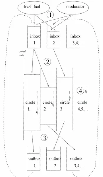
A reactor core is described in a PANTHER model by physical quantities that are homogeneous inside each core volume element (HEX-Z or X-Y-Z). In our shift model we also need the so called box volume elements and rings. A “ring” is a ring of core volume elements that have roughly the same distance to the reactor central axis. Each circulation action is defined per ring. This concerns the top height for the position where new pebbles will be added, the bottom height for the position from where pebbles will be removed, and the vertical shift distance per shift action. An ’inbox’ is a (variable size) volume element containing a mixture of pebbles needed to fill the gaps that arise at the ring tops as a result of a downward shift. This mixture may contain moderator balls and different types of fuel balls of different burn-up classes (including the lowest class, i.e. fresh fuel). An “outbox” is a (variable size) volume element that receives pebbles leaving at the ring bottoms as a result of a downward shift. This may be a mixture of pebbles like that in the
inbox, except that the fuel can not be fresh here; so there are no lowest burn-up class fuel pebbles. Just like the volume elements in the core, the box volume elements contain homogeneous physical quantities, but their sizes are not fixed. Shifting means changing the physical quantities for the volume elements. Each axial shift action moves material from inboxes to rings in the core, per ring over a certain distance downward, and out of these rings to outboxes. Only the basic quantities are always calculated for each volume element directly from shift distances and volume fractions. The other physical quantities are derived from these basic quantities only when needed. For example, the fuel reload decisions need to know the number of fuel pebbles per combination of fuel type and burn-up class only for the box volume elements, not for the core volume elements. The administration for fuel reload decisions is covered by burn-up classes. Therefore the unbound interval of possible burn-up values is divided into a finite number of intervals that cover the total range from 0 to ∞. The lowest class has both upper-bound and lower-upper-bound equal to zero and contains only fresh fuel. The highest class contains all fuel beyond a certain burn-up value limit. The internal composition and the 2 groups cross-sections of a Burn-up class is found with a linear interpolation in the interval of the steps obtained in WIMS calculation [4-5]. WIMS generates also the new homogenized compositions and the homogenized macroscopic cross-sections step per step for a single target (a pebble in a cube with a surround of Helium). With this calculation PANTHERMIX sets the composition of the volume element in function of the burn-up classes in the user input.
4.4.3 Pebble circulation actions
Fig. 4.1 shows the possibilities for pebble circulation actions. The arrows only serve as indicators.
Not all possible routes are shown, and not every arrow represents a route that must always be followed. The pebble circulation actions will now be described according to the encircled numbers in the figure.
1. Fill inboxes (first time empty, later possibly filled to a certain height) with:
o Different type mixtures of fresh fuel: Extra pebbles are added to the system
o Moderator: extra pebbles are added to the system
o Fuel from outboxes: no extra pebbles are added to the system; each inbox may be filled with any amount of any fuel type and burn-up class from any outbox, as long as those pebbles are available in that outbox
Figure 4.1: PANTHERMIX Pebbles recirculation simulator system
2. Connect for each ring that must shift its top to an inbox. The inbox will be called a parent of the ring here. Each ring may have only one inbox as parent. Each inbox may be parent of zero, one or more rings.
3. Connect for each ring that must shift its bottom to an outbox. Here the ring will be called a parent of the outbox. Each ring may be parent of only one outbox. Each outbox may have zero, one or more rings as parent.
4. Shift downwards the contents of each ring over a specified distance. This distance represents the speed of balls through the reactor. The speed in different rings may be different. The figure only shows the downward directed axial speed components, but there may also be inward directed radial speed components. The top and bottom locations do not change height, only the contents between them will change. Details are listed below.
For each shift the new contents of volume elements are mixtures of old volume element contents. An inbox only loses material and energy. If the shift distance does not exceed the axial mesh layer height then a top axial mesh layer becomes a mixture of its old contents and the old contents of an inbox. The other axial mesh layers become mixtures of their old contents and the old contents of the axial mesh layers directly above them. An outbox only receives material and energy, its new content becomes a mixture of its old content and the old contents of some ring bottom layers. If the shift distance does exceed the axial mesh layer height then the mixture ingredients are a bit more complex. All mixtures are calculated with volume weighted averaging. The volume averaging is the governing principle of this calculation; so the two volumes are not necessarily equal. I fact this phenomenon comes down to shifting part of the upper volume (and associated contents) into the lower volume and then "homogenizing" the lower volume. It is important to show that this volume has nothing to do with the way the macroscopic cross section for a volume are being calculated.
4.5 The MonteCarlo method and MCNP5©
MCNP is a general-purpose, continuous-energy, generalized-geometry, time-dependent, coupled neutron/photon/electron MonteCarlo transport code[4-4]. It can be used in several transport modes: neutron only, photon only, electron only, combined neutron/photon transport where the photons are produced by neutron interactions, neutron/photon/electron, photon/electron, or electron/photon reactions. The neutron energy regime is from 10-11 MeV to 20 MeV for all isotopes and up to 150 MeV for some isotopes; the photon energy regime is from 1 keV to 100 GeV, and the electron energy regime is from 1 KeV to 1 GeV. The capability to calculate keff eigenvalues for fissile systems is also a standard feature. The user creates an input file that is subsequently read by MCNP. This file contains information about the problem in areas such as: the geometry specification, the description of materials and selection of cross-section evaluations, the location and characteristics of the neutron, photon, or electron source, the type of answers or tallies desired, and any variance reduction techniques used to improve calculation efficiency. When running a MonteCarlo calculation, it is important to remember the following five “rules’’:
1. Define and sample the geometry and source well. 2. You cannot recover lost information.
3. Question the stability and reliability of results.
5. The number of histories run is not indicative of the quality of the answer.
The following paragraph compares Monte Carlo and deterministic methods and provide a simple description of the Monte Carlo method.
4.6 MonteCarlo method vs. Deterministic method
Monte Carlo methods are very different from deterministic transport methods. Deterministic methods, the most common of which is the discrete ordinates method, solve the transport equation for the average particle behaviour. By contrast, MonteCarlo obtains answers by simulating individual particles and recording some aspects (tallies) of their average behaviour. The average behaviour of particles in the physical system is then inferred (using the central limit theorem) from the average behaviour of the simulated particles. Not only are MonteCarlo and deterministic methods very different ways of solving a problem, even what constitutes a solution is different. Deterministic methods typically give fairly complete information (for example, flux) throughout the phase space of the problem. MonteCarlo supplies information only about specific tallies requested by the user. When MonteCarlo and discrete ordinates methods are compared, it is often said that MonteCarlo solves the integral transport equation, whereas the discrete ordinates method solves the integro-differential transport equation. Two things are misleading about this statement. First, the integral and integro-differential transport equations are two different forms of the same equation; if one is solved, the other is solved. Second, MonteCarlo “solves” a transport problem by simulating particle histories. A transport equation needs not to be written to solve a problem by MonteCarlo. Nonetheless, one can derive an equation that describes the probability density of particles in the phase space; this equation turns out to be the same as the integral transport equation. Without deriving the integral transport equation, it is instructive to investigate why the discrete ordinates method is associated with the integro-differential equation and Monte Carlo with the integral equation. The discrete ordinates method visualizes the phase space to be divided into many small boxes, and the particles move from one box to another. In the limit, as the boxes get progressively smaller, particles moving from box to box take a differential amount of time to move a differential distance in space. In the limit, this approaches the integro-differential transport equation, which has derivatives in space and time. By contrast, MonteCarlo transports particles between events (for example, collisions) that are separated in space and time. Neither differential space nor time are inherent parameters of Monte Carlo transport. The integral equation does not have terms involving time or
space derivatives. MonteCarlo is well suited to solving complicated three-dimensional, usually time-independent problems. Because the MonteCarlo method does not use phase space boxes, there are no averaging approximations required in space, energy, and time. This is especially important in allowing detailed representation of all aspects of physical data. 4.7 The MonteCarlo method
MonteCarlo can be used to reproduce a statistical process (such as the interaction of nuclear particles with materials) and is particularly useful for complex problems that cannot be modelled by computer codes that use deterministic methods [4-4]. The individual probabilistic events that comprise a process are simulated sequentially. The probability distributions governing these events are statistically sampled to describe the total phenomenon. In general, the simulation is performed on a digital computer because the number of trials necessary to adequately describe the phenomenon is usually quite large. The statistical sampling process is based on the selection of random numbers (analogous to throwing dice in a gambling casino), hence the name “Monte Carlo.” In particle transport, the MonteCarlo technique is pre-eminently realistic (a numerical experiment). It consists of actually following each of many particles from a source throughout its life to its death in some terminal category (absorption, escape, etc.). Probability distributions are randomly sampled using transport data to determine the outcome at each step of its life.
Figure 4.2 represents the random history of a neutron incident on a slab of material that can undergo fission. Numbers between 0 and 1 are selected randomly to determine what (if any) and where interaction takes place, based on the rules (physics) and probabilities (transport data) governing the processes and materials involved. In this particular example, a neutron collision occurs at event 1. The neutron is scattered in the direction shown, which is selected randomly from the physical scattering distribution. A photon is also produced and is temporarily stored, or banked, for later analysis. At event 2, fission occurs, resulting in the termination of the incoming neutron and the birth of two outgoing neutrons and one photon. One neutron and the photon are banked for later analysis. The first fission neutron is captured at event 3 and terminated. The banked neutron is now retrieved and, by random sampling, leaks out of the slab at event 4. The fission-produced photon has a collision at event 5 and leaks out at event 6. The remaining photon generated at event 1 is now followed with a capture at event 7. Note that MCNP retrieves banked particles such that the last particle stored in the bank is the first particle taken out. This neutron history is now complete. As more and more such histories are followed, the neutron and photon distributions become better known. The quantities of interest (whatever the user requests) are tallied, along with estimates of the statistical precision (uncertainty) of the results.
4.8 Conclusions
In this chapter we have briefly described the PANTHERMIX and the MCNP5© codes, that were used in combination, in order to calculate, using MCNP5©, some pebble conditions that are out of linear behaviour, not suitable of solution by PANTHERMIX (see Chapter 5). The use of MCNP has allowed to produce data in order to write a new Mixing Model able to correct the older one.
![Figure 4.2: Random history of a neutron incident in a fissionable material[4-4]](https://thumb-eu.123doks.com/thumbv2/123dokorg/7323014.89820/9.892.106.805.751.1133/figure-random-history-neutron-incident-fissionable-material.webp)