A topological approach for multivariate time series characterization: the epileptic brain

(1)

A topological approach for multivariate time series

characterization: the epileptic brain

Emanuela Merelli, Marco Piangerelli, Matteo Rucco, Daniele Toller

Computer Science Division University of Camerino

{emanuela.merelli, marco.piangerelli, matteo.rucco, daniele.toller}@unicam.it

ABSTRACT

In this paper we propose a methodology based on Topogical Data Analysis (TDA) for capturing when a complex system, represented by a multivariate time series, changes its inter-nal organization. The modification of the inner organization among the entities belonging to a complex system can induce a phase transition of the entire system. In order to identify these reorganizations, we designed a new methodology that is based on the representation of time series by simplicial complexes. The topologization of multivariate time series successfully pinpoints out when a complex system evolves. Simplicial complexes are characterized by persistent homo-logy techniques, such as the clique weight rank persistent homology and the topological invariants are used for com-puting a new entropy measure, the so-called weighted per-sistent entropy. With respect to the global invariants, e.g. the Betti numbers, the entropy takes into account also the topological noise and then it captures when a phase transi-tion happens in a system. In order to verify the reliability of the methodology, we have analyzed the EEG signals of Phy-sioNet database and we have found numerical evidences that the methodology is able to detect the transition between the pre-ictal and ictal states.

Categories and Subject Descriptors

D.2.8 [Software Engineering]: Metrics—complexity mea-sures, performance measures; G.3 [Probability and Statis-tics]: Miscellaneous; H.4 [Information Systems Appli-cations]: Miscellaneous

General Terms

Theory

Keywords

Topological Data Analysis, Multivariate Time Series, Com-plex Systems, Epilepsy, Entropy, Signal Analysis

.

1. INTRODUCTION

A complex system can be generally described as a dynami-cal system composed by a huge number of autonomous, but interrelated and interdependent, entities that can be linked both functionally and spatially. The dynamic linking forms a dense network of interactions. Complex systems cannot be decomposed by a single rule and their properties can not be reduced to one level of description. They are in general characterized by emerging features and behaviors that arise from the interaction of their parts and cannot be predicted from the properties of the parts. The science of complex-ity deals with the following questions: how interactions give rise to new unobserved behaviors and how to model complex systems. In the past, two approaches were used for studying complex systems: agent based model and simulation and dif-ferential equations (both ordinary and partial). Because the increasing of data volume associated to complex systems, actually, two alternatives approaches are used: multivariate time series [16] and complex networks [1]. In this paper we intend to provide a methodology for representing complex systems by multivariate time series and transforming the signals into complex networks that are analyzed by topolog-ical data analysis (TDA) and information theory [19, 15]. In order to minimize the effect of the noise in the signals and to produce equivalence classes among patterns in the EEG time series we segmented the multivariate time series. TDA is an innovative approach for dealing with big-data, it allows us to perform data-space reduction, and to identify the higher order relations existing among the entities of a complex system [7]. TDA has been largely used in several fields, spanning from biology to social networks [14, 4]. The paper is organized as follows: in Section 2 we introduce the biological case study, in Section 3 we describe the method-ology, in Section 4 we briefly remark the maths behind the methodology and in Sections 6 and 7 we discuss the out-comes.

2. CASE STUDY: EPILEPTIC BRAIN

Epilepsy is a chronic disorder of the brain that affects people all over the world. It is characterized by recurrent seizures, which are brief involuntary movements involving a part of the body (partial) or the whole body (generalized). Some episodes can be accompanied of loss of consciousness and control living functions1. Epileptic seizures are defined as sudden interruptions of brain functions due to an abnor-mal, excessive or synchronous activity of a neuronal

ensem-1

http://www.who.int/en/

(2)

ble. Most of the people affected by epilepsy can control it by assuming anti-epileptic drugs, about 30% [2] of the epilep-tic patients are drug-resistant: 60% of them can undergo resection surgery, for the others alternative therapies, such as devices capable to predict the onset of epileptic seizures thus controlling them, have to be taken into account. In de-veloping devices, it is fundamental cosidering that brain is a complex self-adaptive system. The brain dynamics under-goes through several phase transitions generating complex behaviors [17, 8]. This is the reason why the study of time-varying brain signals, such as EEG (or intracranical elec-troencephalography (iEEG)), functional magnetic resonance imaging (fMRI) and magnetoencephalography (MEG), is both the key-aspect for finding new insights and the highest barrier. In studying epilepsy, one of the main open ques-tion is the definiques-tion of the so-called pre-ictal state, i.e. the state before the onset of an epilepetic seizure, which is the ictal state, and the detection of the phase transition between the two states. In the last years, several studies based on non-linear analysis proved that the transtion between the pre-ictal and the ictal state is not an abrupt change [11, 9]. This outcame suggests that the detection of the pre-ictal state minutes or hours before the onset of an epileptic seizure can be possible. Assessing the pre-ictal state (and its features) and the transient pre-ictal to ictal can be crucial in understandng the underlying transition mechanisms and the ictogenesis which are necessary in developing prediction algorithms [10]. The study of epilepsy as a complex dy-namical system can be faced up by analyzing the EEG time series. As far as we know, there is not a universal machin-ery able to identify the onset of the phenomena, due to the subjectivity of the crisis and the noise affecting the signal; however in the past decades, several attempts were made: linear and non linear analysis, univariate and multivariate techniques, as well as methods from different scientific fields such as time-frequency domain, dynamical system domain, chaos theory and even graph theory [17, 13].

3. METHODOLOGY

Complex dynamical systems arise as mathematical de-scriptions of natural phenomena. Studying the time evo-lution of such systems provides broad insight into problems. A wide spectrum of behaviors is seen, from straightforward limit cycles to chaotic behavior stemming from sensitivity to initial conditions. However, nature is affected by noise that often obfuscates the true behaviors. In order to cap-ture the behavior, we intend to represent the system by sim-plicial complexes. The construction of simsim-plicial complexes from real data is only partially affected by the noise, while the topological invariants (i.e., the Betti numbers) are pre-served [6]. The protocol we propose consists in the following steps:

1. Segmenting the multivariate time series. The length of the windows is driven by the method proposed by [18] or similar approaches.

2. For each window, compute the Pearson correlation co-efficients (or partial correlation) matrix ρ(i, j). 3. Threshold the matrix by selecting the correlation

co-efficient statistically significant (p − value < 0.05) and greater than a threshold θ = 0 ρ(i, j) > θ.

4. Represent the thresholded matrix as a weighted edge list.

5. Use jHoles for computing clique weight rank persistent homology.

6. Compute and plot the weighted persistent entropy.

4. SIMPLICIAL COMPLEXES

A simplicial complex is a mathematical object used to generalize the idea of a triangulation of a surface. It is made of assembling units called simplices, glued together following some rules we shall see in a while.

For an integer n ∈ N, an n-dimensional simplex is the con-vex hull of n + 1 points in general position. For example, a 0-dimensional simplex is just a single point; a 1-dimensional simplex is a segment (containing both its ending points, that are the two 0-simplices that determine it); a 2-dimensional simplex is a triangle: it is determined by its three vertices (0-simplices) say A, B, C, and consists of the closed area deli-mited by its three edges AB, BC, AC, which themselves are 1-simplices. Similarly, a 3-dimensional simplex is a generic tetrahedron: it has four 0-simplices, six 1-simplices, and four 2-simplices (the triangles that constitute its surface). Note that given an n-dimensional simplex S (i.e. n + 1 points determining it), every subset of k + 1 ≤ n + 1 points is itself a k-dimensional simplex T ; in this situation, we say that the subcomplex T ⊆ S is a subface of S. Then a simplicial com-plex is a family K of comcom-plexes with the properties that: (1) every subcomplex of a member of K is still a member of K, and (2) the intersection of two complexes in K is again in K. These two requests essentially prevent complexes ‘to have no borders’ (condition (1)), and tell how to glue simplexes together to form a complex (condition (2)): they are allowed only to share an entire common subface. The dimension of a simplicial complex is the maximum among the dimensions of its complexes. For example, a 0-dimensional simplicial complex is just a collection of points, while a 1-dimensional simplicial complex is a collection of points with some seg-ments connecting some of them, i.e. it is nothing more than a graph. A filtered simplicial complex (or a filtration on a simplicial complex) is a finite, ordered, family of simplicial complexes, each of them contained in the previous one; one can intuitively think of it as the finite time steps required to build the last, final, simplicial complex. Given a weighted graph, there are several ways to make a filtered simplicial complex out of it; here we expose the clique weight rank pro-cedure, implemented by the jHoles software [3]. First, we look for the maximal cliques (i.e. complete subgraphs) in the graph. For each of them, we note its cardinality, say n, and we add to our simplicial complex the (n−1)-dimensional complex determined by its points, as well as all of its sub-faces (i.e. subcomplexes, i.e. subcliques). Then, we look for the (n − 1)-cliques that are not already been considered (i.e. that are not contained in any previous found n-clique), and we proceed as before. In the meantime, when we find a maximal clique, we attribute a weight to it, namely the minimum among the weights of the edges in the clique, and this value will be used to decide at which step of the filtered simplicial complex the clique will appear.

The upper part of Figure 1 shows an example of this pro-cedure. The weights of the edges of the starting graph are listed in the set W in increasing order.

(3)

Figure 1: Example of clique weight rank persistent homology. Top: clique complexes construction from a weighted undirected graph. The maximal cliques are listed by the Bron-Kerbosch algorithm. Bottom: Betti barcodes obtained during the computation of persistent homology [7].

4.1 Homology, persistent homology and

bar-codes

The homology of a simplicial complex, and the persistent homology of a filtered simplicial complex, are very effec-tive methods to study networks and to discover relations between nodes in them. The explicit definition of these ob-jects is beyond the scope of this paper, and here we only give an intuitive idea of them, that will suffice for making this paper self-consistent. Given a filtered simplicial complex of dimension d ∈ N, let F be the set of its filtration values. For every j ≤ d, the software jHoles computes the so-called ho-mology group Hj, whose elements are called j-dimensional

cycles. Each cycle is also equipped with an interval (also called line) of the form either [a, b] or [a, ∞) for a, b filtration values, that represents the filtration values of birth (time a) and death (time b, or ∞) of the cycle. Intervals of the form [a, b] correspond to topological noise; while [a, ∞) represents a persistent topological feature (a cycle that is born at time a and dies at time ∞). If m = max{F } + 1, from now on we will denote by [a, m] such an otherwise unbounded interval: from the point of view of the filtration F , saying that a cycle stands up to time m or up to time ∞ is the same. The union of the lines associated to j-dimensional cycles is called j-th Betti barcode. The “infinite” persistent barcodes represent the persistent Betti numbers βi, i ∈ N.

5.

J

-WEIGHTED PERSISTENT ENTROPIES

Let d be the dimension of the simplicial complex. For every j ∈ N, j ≤ d, we consider the j-th homology space Hj,

and let Njbe the number of lines (both noise and persistent

topological features) belonging to Hj. We set li= (bi− ai)

to be the length of the i-th topological feature belonging to Hj. Now we let Lj = Σ

Nj

i=1li be the total length of the

j-th barcode, and Pi = _Lli

j be the frequential probability

for li and Lj. Finally, we define the j-Weighted Persistent

Entropy W Hjthat is an extension of the Persistent Entropy

H defined in [5] as W Hj= −cjΣ

Nj

i=1P (li) · log(P (li)). (1)

where cj = 2j. Note that two are the main differences

be-tween H and W Hj: the latter is computed for each j-th

homological space, while H is computed over the entire set of lines. The second difference is in the cjcoefficient: it

em-phasize the contribution of higher Homological groups on the entropy. Note that if N = 1, then the entropy is 0, while it can be proved that if N > 1 then the entropy value is maximum if the barcode is formed by lines having the same length.

6. RESULTS

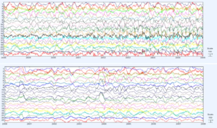
In this section we report on the application of the method-ology described in Section 3 to the EEG signals stored in the PhysioNet database and freely accesible by the web-site2. The EEG signals used in this study were collected at the Children’s Hospital Boston, and they consists of EEG recordings from pediatric subjects with intractable seizures. Subjects were monitored for up to several days following withdrawal of anti-seizure medication in order to charac-terize their seizures and assess their candidacy for surgical intervention. Because of the limitation on the number of pages, we report only on two signals, respectively sigI and sigII (see Figure 2). We applied the procedure described

Figure 2: Example of EEG signals: sigI is on the top, while sigII is on the bottom

in [18] to both signals and we found the optimal size of the segmentation is equal to 120secs, then we segmented the whole ECG track in 30 windows. For each window we computed the partial correlation coefficients and we used as threshold θ = 0. The upper triangular part of each matrices was parsed and saved as edge list, hence the edge list was used as input for jHoles. jHoles provides the Betti barcodes both in graphical and textual formats, and we used the lat-ter for computing the weighted persistent entropy over each homological dimension (H0, H1, H2, and H3). We plotted

the W Hj values for each matrix (see Figure 3).

7. CONCLUSIONS

2

(4)

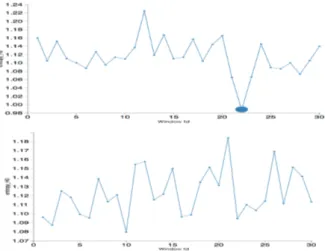
Figure 3: Weighted Persistent Entropy for the ho-mological group H0. Top: Weighted persistent

en-tropy for the sigI, the marked peak corresponds to an ictal state. Bottom: Weighted persistent entropy for the sigII. In the upper figure a phase transition is well evident.

The two signals have been previously classified by the Phy-sioNet users. Respectively, sigI corresponds to an individ-ual affected by epilepsy, while sigII belongs to an healthy patient. This classification also is identified by our metho-dology. The analysis of the persistent entropy reveals that in W H0 of sigI a phase transition occurs (see the upper

picture in Figure 3). The topological interpretation is that among the windows with id = 20, 21 and 22, the number of connected components tends to be one and the topological noise is minimized (all the features are persistent). Before and after this period, the number of connected component is higher and the barcodes are noisy. These three windows correspond exactly to the transition from the pre-ictal state to the ictal state. In both signals, Betti numbers for higher dimensions are present (β1, β2, β3) but in these signals the

corresponding barcodes do not change significantly. As fu-ture work we plan to use this methodology and to investigate this kind of natural complex phenomena by following the S[B] paradigm. S[B] allows to model simultaneously both the local and the global behaviors of complex systems [12].

8. ACKNOWLEDGMENTS

We acknowledge the financial support of the Future and Emerging Technologies (FET) programme within the Sev-enth Framework Programme (FP7) for Research of the European Commission, under the FP7 FETProactive Call 8 -DyMCS, Grant Agreement TOPDRIM, number FP7-ICT-318121.

9. REFERENCES

[1] R. Albert and A.-L. Barab´asi. Statistical mechanics of complex networks. Reviews of modern physics, 74(1):47, 2002.

[2] P. N. Banerjee, D. Filippi, and W. Allen Hauser. The descriptive epidemiology of epilepsy—A review. Epilepsy Research, 85(1):31–45, July 2009. [3] J. Binchi, E. Merelli, M. Rucco, G. Petri, and

F. Vaccarino. jholes: A tool for understanding

biological complex networks via clique weight rank persistent homology. Electronic Notes in Theoretical Computer Science, 306:5–18, 2014.

[4] C. Carstens and K. Horadam. Persistent homology of collaboration networks. Mathematical Problems in Engineering, 2013, 2013.

[5] F. Castiglione, E. Merelli, M. Pettini, and M. Rucco. Correlation between topological complexity and entropy in idiotypic network. 2014.

[6] A. Chernov and V. Kurlin. Reconstructing persistent graph structures from noisy images. Image-a.= Imagen-a., 3(5):19–22, 2013.

[7] H. Edelsbrunner and J. Harer. Persistent homology-a survey. Contemporary mathematics, 453:257–282, 2008.

[8] L. D. Iasemidis and J. C. Sackellares. REVIEW : Chaos Theory and Epilepsy. The Neuroscientist, 2(Ldi):118–126, 1996.

[9] M. Le Van Quyen, J. Martinerie, M. Baulac, and F. Varela. Anticipating epileptic seizures in real time by a non-linear analysis of similarity between EEG recordings. Technical Report 10, Laboratoire de Neurosciences Cognitives et Imagerie Cérébrale (CNRS UPR 640) and Unité D’epileptologie, Hôpital de la Salpêtrière, Paris, France., 1999.

[10] M. Le Van Quyen, J. Soss, V. Navarro, R. Robertson, M. Chavez, M. Baulac, and J. Martinerie. Preictal state identification by synchronization changes in long-term intracranial EEG recordings. Clinical Neurophysiology, 116:559–568, 2005.

[11] B. Litt, R. Esteller, J. Echauz, M. D’Alessandro, R. Shor, T. Henry, P. Pennell, C. Epstein, R. Bakay, M. Dichter, and G. Vachtsevanos. Epileptic seizures may begin hours in advance of clinical onset: A report of five patients. Neuron, 30(1):51–64, 2001.

[12] E. Merelli, N. Paoletti, and L. Tesei. A multi-level model for self-adaptive systems. arXiv preprint arXiv:1209.1628, 2012.

[13] L. Orosco. Review: A Survey of Performance and Techniques for Automatic Epilepsy Detection. Journal of Medical and Biological Engineering, 33(6):526, 2013. [14] G. Petri, P. Expert, F. Turkheimer, R. Carhart-Harris,

D. Nutt, P. Hellyer, and F. Vaccarino. Homological scaffolds of brain functional networks. Journal of The Royal Society Interface, 11(101):20140873, 2014. [15] R. Quax. Information processing in complex networks.

network, 71:151, 2013.

[16] J. C. Sprott and J. C. Sprott. Chaos and time-series analysis, volume 69. Oxford University Press Oxford, 2003.

[17] Q. K. Telesford, S. L. Simpson, J. H. Burdette, S. Hayasaka, and P. J. Laurienti. The Brain as a Complex System: Using Network Science as a Tool for Understanding the Brain. Brain Connectivity,

1(4):295–308, Oct. 2011.

[18] Y. Yang and H. Yang. Complex network-based time series analysis. Physica A: Statistical Mechanics and its Applications, 387(5-6):1381–1386, Feb. 2008. [19] A. Zomorodian and G. Carlsson. Computing

persistent homology. Discrete & Computational Geometry, 33(2):249–274, 2005.