POLITECNICO DI MILANO
Scuola di Ingegneria Industriale e dell’Informazione
Dipartimento di Chimica, Materiali e Ingegneria Chimica “Giulio Natta”
Corso di Laurea Magistrale in Ingegneria Chimica
A hybrid economic/econometric model of crude oil prices
for PSE/CAPE applications under historical fluctuations and
market uncertainties
Relatore: Prof. Davide MANCA
Tesi di Laurea Magistrale di:
Valentina DEPETRI
matr. 813268
“Don’t never prophesy: If you prophesies right, ain’t nobody going to remember and if you prophesies wrong, ain’t nobody going to let you forget”
1
Contents
Figures... 5 Tables ... 11 Acronyms ... 13 Abstract (English) ... 15 Abstract (Italian) ... 17Introduction and aim of the work ... 19
Motivation and structure of the work ... 20
Chapter 1 Historical background ... 25
1.1 Introduction to recent historical trends of crude oil quotations... 25
1.1.1 The 2008 crude oil price crash ... 28
1.1.2 WTI and Brent divergence and shale oil “revolution” ... 29
1.1.3 The last price crash in December 2014 ... 34
1.1.4 Very recent events: Greek crisis, withdrawal of Iranian embargo, and Chinese crisis of stock exchanges ... 35
1.2 The crude oil market ... 37
Chapter 2 Literature overview ... 51
2.1 An insight into market, price, and volatility of crude oil ... 51
2.2 Crude oil models classification... 55
Chapter 3 Econometric models ... 59
3.1 Introduction to time series analysis ... 59
3.1.1 Modeling financial time series by means of econometric models ... 60
3.1.1.1 ARMA model ... 61
2
3.1.1.5 GJR-GARCH model ... 64
3.1.1.6 APARCH model ... 64
3.1.2 General methodology and statistical tools... 65
3.1.2.1 Time plot ... 65
3.1.2.2 Measures of skewness and kurtosis ... 65
3.1.2.3 Jarque-Bera test ... 68
3.1.2.4 Correlation and autocorrelation function ... 69
3.2 Statistical analysis and results of price and volatility of crude oil ... 70
3.3 Random walk model ... 76
Chapter 4 Economic models ... 81
4.1 Introduction to the general features and issues of economic models ... 81
4.2 Ye’s model ... 82
4.2.1 A brief literature review ... 82
4.2.2 Determining fundamental factors: the role of inventory level and excess production capacity in economic models ... 83
4.2.3 Model description and simulation... 85
4.3 Chevallier’s model ... 88
4.3.1 Determining fundamental factors: physical, economic, and financial variables .... 88
4.3.2 Model description ... 90
4.3.2.1 Disaggregated CFTC data ... 91
4.3.3 Simulation of a new model inspired by Chevallier (2014) ... 91
Chapter 5 A new OPEC-based model for PSE applications ... 97
5.1 Historical review of OPEC behavior ... 97
3
5.1.2 OPEC behavior and price trend ... 105
5.2 Models description ... 106
5.2.1 Economic models inspired by the behavior of OPEC ... 106
5.2.2 New economic crude oil price model ... 108
5.2.3 Input variable models ... 117
5.2.3.1 OECD demand ... 121
5.2.3.2 OECD inventories ... 125
5.2.3.3 OPEC production ... 128
5.2.3.4 OPEC production capacity ... 131
5.2.3.5 USA production ... 133
5.2.3.6 OPEC quotas ... 137
5.2.4 Model identifiability ... 138
5.2.4.1 The concept of identifiability ... 139
5.2.4.2 Fisher Information Matrix ... 140
5.2.4.3 A differential algebra approach: DAISY algorithm ... 142
5.2.5 Sensitivity analysis ... 145
5.2.5.1 Parametric sensitivity ... 146
5.2.5.2 Input variables sensitivity ... 149
5.2.6 Model validation and selection of the forecast horizon ... 153
5.3 Model simulations: the creation of fully predictive scenarios ... 159
5.4 Model manipulation: bullish, bearish, and “neutral” scenarios ... 168
Chapter 6 Development and simulation of crude oil price hybrid model ... 173
6.1 Why a hybrid model ... 173
6.1.1 Econometric model description ... 175
4
Conclusions and future developments ... 183
Appendix A ... 187
A.1 Brent price ... 187
A.2 WTI price ... 189
A.3 OECD demand ... 191
A.4 OECD inventories ... 192
A.5 OPEC production ... 193
A.6 OPEC production capacity ... 194
A.7 USA production ... 195
A.8 Model parameters ... 196
Appendix B ... 199
B.1 Fisher information matrix ... 199
Appendix C ... 201
C.1 DAISY input file ... 201
C.2 DAISY output file ... 202
References ... 205
5
Figures
Figure 1 - Crude oil reserves and production of major refining companies (data taken from Agnoli,
2014). ... 27
Figure 2 - Capital expenditures of major refining companies (data taken from Elliott, 2015). ... 27
Figure 3 - Brent and WTI monthly quotations from Jan, 1996 to Apr, 2015 (data from EIA). ... 29
Figure 4 - Brent-WTI differential values between Brent and WTI monthly quotations (data from EIA)……… 30
Figure 5 - Internal combustion technology for shale oil extraction and scheme of a vertical shaft retort. ... 32
Figure 6 - In situ extraction of shale oil. ... 32
Figure 7 - US crude oil annual production and net imports from 1920 to 2010 (data from EIA). ... 33
Figure 8 - Comparison between the USA crude oil production and Saudi Arabia production from Feb, 2008 to Feb, 2015 (quarterly data from EIA). ... 33
Figure 9 - Brent and WTI crude oil monthly quotations from Jan, 2014 to Apr, 2015 (data from EIA). 34 Figure 10 - OPEC exports by destination in 2013 (data taken from BP, 2014). ... 38
Figure 11 - Global proved reserves in 1998 (data taken from BP, 2014). ... 39
Figure 12 - Global proved reserves in 2013 (data taken from BP, 2014). ... 39
Figure 13 - OPEC proved reserves in 1998 (data taken from BP, 2014). ... 40
Figure 14 - OPEC proved reserves in 2013 (data taken from BP, 2014). ... 40
Figure 15 - OECD proved reserves in 1998 (data taken from BP, 2014). ... 41
Figure 16 - OECD proved reserves in 2013 (data taken from BP, 2014). ... 41
Figure 17 - BRIC proved reserves in 1998 (data taken from BP, 2014). ... 41
Figure 18 - BRIC proved reserves in 2013 (data taken from BP, 2014). ... 42
Figure 19 - Global crude oil production in 1998 (data taken from BP, 2014). ... 42
Figure 20 - Global crude oil production in 2013 (data taken from BP, 2014). ... 43
Figure 21 - BRIC crude oil production in 1998 (data taken from BP, 2014). ... 43
Figure 22 - BRIC crude oil production in 2013 (data taken from BP, 2014). ... 43
Figure 23 - OECD crude oil production in 1998 (data taken from BP, 2014). ... 44
Figure 24 - OECD crude oil production in 2013 (data taken from BP, 2014). ... 44
Figure 25 - OPEC crude oil production in 1998 (data taken from BP, 2014). ... 45
Figure 26 - OPEC crude oil production in 2013 (data taken from BP, 2014). ... 45
Figure 27 - Global crude oil consumption in 1998 (data taken from BP, 2014). ... 46
Figure 28 - Global crude oil consumption in 2013 (data taken from BP, 2014). ... 46
Figure 29 - BRIC crude oil consumption in 1998 (data taken from BP, 2014). ... 46
Figure 30 - BRIC crude oil consumption in 2013 (data taken from BP, 2014). ... 47
Figure 31 - OECD crude oil consumption in 1998 (data taken from BP, 2014). ... 47
Figure 32 - OECD crude oil consumption in 2013 (data taken from BP, 2014). ... 48
Figure 33 - Global refinery capacity in 1998 (data taken from BP, 2014). ... 48
Figure 34 - Global refinery capacity in 2013 (data taken from BP, 2014). ... 49
Figure 35 - OECD refinery capacity in 1998 (data taken from BP, 2014). ... 49
6
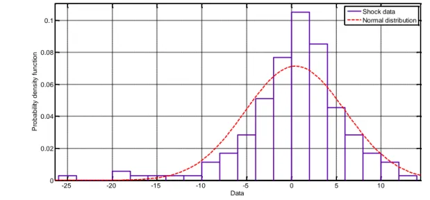
Figure 40 - Histogram for 10000 Weibull random numbers. ... 68 Figure 41 - Brent monthly shocks from 2000 to 2014. ... 70 Figure 42 - Brent monthly relative shocks from 2000 to 2014... 71 Figure 43 - Autocorrelogram of WTI shocks on monthly basis (data from Jan, 2009 to Aug, 2014). .... 73 Figure 44 - Autocorrelogram of WTI relative shocks on monthly basis (data from Jan, 2009 to Aug, 2014). ... 73 Figure 45 - Comparison between histogram of shock data and the normal distribution. ... 74 Figure 46 - Comparison between the cumulative frequency functions of shock data and normal distribution... 75 Figure 47 - Comparison between histogram of relative shock data and the normal distribution. ... 75 Figure 48 - Comparison between the cumulative frequency functions of relative shock data and normal distribution. ... 76 Figure 49 - Brent prices from 2009 to 2019: the period from November, 2014 to November, 2019 represents the forecast range (100 different simulations for 60 months). ... 78 Figure 50 - WTI prices from 2009 to 2019: the period from November, 2014 to November, 2019
represents the forecast range (100 different simulations for 60 months). ... 79 Figure 51 - Fan-chart of Brent prices from 2009 to 2019: the period from November, 2014 to November, 2019 represents the forecast range (100 different simulations) with probability from 0.1% (darker green) to 99.9% (lighter green). ... 79 Figure 52 - Fan-chart of WTI prices from 2009 to 2019: the period from November, 2014 to November, 2019 represents the forecast range (100 different simulations) with probability from 0.1% (darker green) to 99.9% (lighter green). ... 80 Figure 53 - WTI price simulations on monthly basis with one-step-ahead (red solid line) and
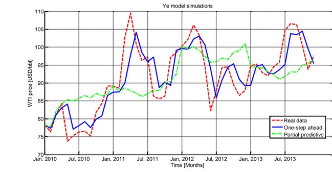
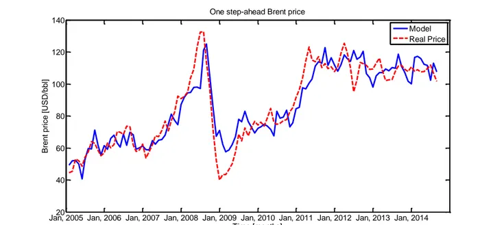
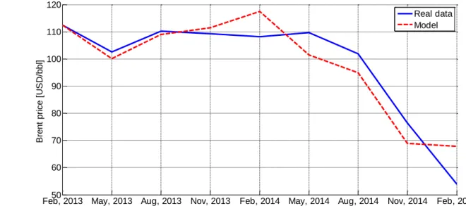
partial-predictive (green dotted line). ... 87 Figure 54 - One-step-ahead simulation of Brent monthly prices from January, 2005 to August, 2014 (real data from EIA). ... 94 Figure 55 - Partial-predictive forecast scenarios and real Brent monthly prices (red solid line) from January, 2005 to August, 2014 (real data from EIA). ... 94 Figure 56 - One-step-ahead simulation of WTI monthly prices from January, 2005 to August, 2014 (real data from EIA). ... 95 Figure 57 - Partial-predictive forecast scenarios and real WTI monthly prices (red solid line) from January, 2005 to August, 2014 (real data from EIA). ... 95 Figure 58 - Historical crude oil yearly price data from 1861 to 2014 with the current USD value and the money value of that year (data taken from BP, 2014). ... 99 Figure 59 - OPEC deviation from quota (data from EIA, 2014). ... 103 Figure 60 - 3D plots of (a) Brent price, Days, and Cheat; (b) Brent price, Cheat, and Caputil; (c) Brent price, Days, and Caputil; (d) Brent price, Cheat, and Delta; (e) Brent price, Delta, and Caputil; (f) Brent price, Days, and Delta. ... 110 Figure 61 - One-step-ahead simulation of Brent quarterly prices from Feb, 2013 to Feb, 2015 (real data from EIA). ... 111
7 Figure 62 - One-step-ahead simulation of WTI quarterly prices from Feb, 2013 to Feb, 2015 (real data
from EIA). ... 112
Figure 63 - values for each eight quarter-long simulation. ... 112
Figure 64 - values for each eight quarter-long simulation. ... 113
Figure 65 - values for each eight quarter-long simulation. ... 113
Figure 66 - values for each eight quarter-long simulation. ... 114
Figure 67 - values for each eight quarter-long simulation. ... 114
Figure 68 - values for each eight quarter-long simulation. ... 115
Figure 69 - OECD demand and OPEC production from the first quarter of 2008 to the first quarter of 2015 (data from EIA). ... 119
Figure 70 - Normalized OECD demand and normalized OPEC production from the first quarter of 2008 to the first quarter of 2015. ... 119
Figure 71 - OECD inventories from the first quarter of 2008 to the first quarter of 2015 (data from EIA). ... 120
Figure 72 - OPEC production, OPEC production capacity, and OPEC quota from the first quarter of 2008 to the first quarter of 2015 (data from EIA). ... 120
Figure 73 - Comparison of the Boolean variables adaptive coefficients for demand model... 122
Figure 74 - One-step-ahead simulation of quarterly OECD crude oil demand from Aug, 2012 to Aug, 2014 (real data from EIA). ... 123
Figure 75 - One-step-ahead simulation of quarterly OECD crude oil demand from Nov, 2012 to Nov, 2014 (real data from EIA). ... 124
Figure 76 - One-step-ahead simulation of quarterly OECD crude oil demand from Feb, 2013 to Feb, 2015 (real data from EIA). ... 124
Figure 77 - Schematic representation of the inventory concept. ... 125
Figure 78 - One-step-ahead simulation of quarterly OECD crude oil inventories from Aug, 2012 to Aug, 2014 (real data from EIA). ... 127
Figure 79 - One-step-ahead simulation of quarterly OECD crude oil inventories from Nov, 2012 to Nov, 2014 (real data from EIA). ... 127
Figure 80 - One-step-ahead simulation of quarterly OECD crude oil inventories from Feb, 2013 to Feb, 2015 (real data from EIA). ... 128
Figure 81 - One-step-ahead simulation of quarterly OPEC production from Aug, 2012 to Aug, 2014 (real data from EIA). ... 130
Figure 82 - One-step-ahead simulation of quarterly OPEC production from Nov, 2012 to Nov, 2014 (real data from EIA). ... 130
Figure 83 - One-step-ahead simulation of quarterly OPEC production from Feb, 2013 to Feb, 2015 (real data from EIA). ... 131
Figure 84 - One-step-ahead simulation of quarterly OPEC production capacity from Aug, 2012 to Aug, 2014 (real data from EIA). ... 132
Figure 85 - One-step-ahead simulation of quarterly OPEC production capacity from Nov, 2012 to Feb, 2014 (real data from EIA). ... 133
Figure 86 - One-step-ahead simulation of quarterly OPEC production capacity from Feb, 2013 to Feb, 2015 (real data from EIA). ... 133
Figure 87 - One-step-ahead simulation of quarterly USA production from Aug, 2012 to Aug, 2014 (real data from EIA). ... 136
8
data from EIA). ... 137 Figure 90 - Sensitivity analysis of the price model respect to the adaptive parameter . The adopted values of the input variables are in ascending order for cyan, red, and blue lines. ... 146 Figure 91 - Sensitivity analysis of the price model respect to the adaptive parameter . The adopted values of the input variables are in ascending order for cyan, red, and blue lines. ... 147 Figure 92 - Sensitivity analysis of the price model respect to the adaptive parameter . The adopted values of the input variables are in ascending order for cyan, red, and blue lines. ... 147 Figure 93 - Sensitivity analysis of the price model respect to the adaptive parameter . The adopted values of the input variables are in ascending order for cyan, red, and blue lines. ... 148 Figure 94 - Sensitivity analysis of the price model respect to the adaptive parameter . The adopted values of the input variables are in ascending order for cyan, red, and blue lines. ... 148 Figure 95 - Sensitivity analysis of the price model respect to the adaptive parameter . The adopted values of the input variables are in ascending order for cyan, red, and blue lines. ... 149 Figure 96 - Sensitivity analysis of the price model respect to OECD demand. The adopted values of the input variables are in ascending order for cyan, red, and blue lines. ... 150 Figure 97 - Sensitivity analysis of the price model respect to OPEC production. The adopted values of the input variables are in ascending order for cyan, red, and blue lines. ... 151 Figure 98 - Sensitivity analysis of the price model respect to OECD inventories. The adopted values of the input variables are in ascending order for cyan, red, and blue lines. ... 151 Figure 99 - Sensitivity analysis of the price model respect to OPEC production capacity. The adopted values of the input variables are in ascending order for cyan, red, and blue lines. ... 152 Figure 100 - Sensitivity analysis of the price model respect to USA production. The adopted values of the input variables are in ascending order for cyan, red, and blue lines. ... 152 Figure 101 - Sensitivity analysis of the price model respect to OPEC quota. The adopted values of the input variables are in ascending order for cyan, red, and blue lines. ... 153 Figure 102 - Fully-predictive scenarios of Brent quarterly prices from Feb, 2012 to Feb, 2015. The green dotted line represents the real quotations (real data from EIA). ... 154 Figure 103 - Fully-predictive scenarios of Brent quarterly prices from Feb, 2013 to Feb, 2015. The green dotted line represents the real quotations (real data from EIA). ... 154 Figure 104 - Fully-predictive scenarios of Brent quarterly prices from Feb, 2014 to Feb, 2015. The green dotted line represents the real quotations (real data from EIA). ... 155 Figure 105 - Fully-predictive scenarios of Brent quarterly prices that go past the 150 USD/bbl threshold in May, 2014 and Nov, 2014. The red dash-dot line represents the price level of 150 USD/bbl which is practically the maximum value of CO quotations and took place in July, 2008. ... 156 Figure 106 - Fully-predictive scenarios of OECD quarterly demand from Feb, 2013 to Feb, 2015. The green dotted line represents the real demand (real data from EIA). ... 157 Figure 107 - Fully-predictive scenarios of OECD quarterly inventories from Feb, 2013 to Feb, 2015. The green dotted line represents the real inventories (real data from EIA). ... 157 Figure 108- Fully-predictive scenarios of OPEC production capacity from Feb, 2013 to Feb, 2015. The green dotted line represents the real capacity (real data from EIA). ... 158
9 Figure 109 - Fully-predictive scenarios of OPEC production from Feb, 2013 to Feb, 2015. The green dotted line represents the real OPEC production (real data from EIA). ... 158 Figure 110 - Fully-predictive scenarios of USA production from Feb, 2013 to Feb, 2015. The green dotted line represents the real USA production (real data from EIA). ... 159 Figure 111 - Fully-predictive scenarios of Brent quarterly quotations from Feb, 2015 to Feb, 2017 (3000 simulations over 8 quarters). The yellow dotted line is the average forecast price……….. 161 Figure 112 - Fully-predictive scenarios of WTI quarterly quotations from Feb, 2015 to Feb, 2017 (3000 simulations over 8 quarters). The yellow dotted line is the average forecast price. ... 162 Figure 113 - Fully-predictive scenarios of OECD quarterly demand from Feb, 2015 to Feb, 2017 (3000 simulations over 8 quarters). The yellow dotted line is the average forecast demand. 162 Figure 114 - Fully-predictive scenarios of OECD quarterly inventories from Feb, 2015 to Feb, 2017 (3000 simulations over 8 quarters). The yellow dotted line is the average forecast inventories. ... 163 Figure 115 - Fully-predictive scenarios of OPEC quarterly production from Feb, 2015 to Feb, 2017 (3000 simulations over 8 quarters). The yellow dotted line is the average forecast production. ... 163 Figure 116 - Fully-predictive scenarios of OPEC quarterly production capacity from Feb, 2015 to Feb, 2017 (3000 simulations over 8 quarters). The yellow dotted line is the average forecast production capacity. ... 164 Figure 117 - Fully-predictive scenarios of USA quarterly production from Feb, 2015 to Feb, 2017 (3000 simulations over 8 quarters). The yellow dotted line is the average forecast production. ... 164 Figure 118 - Brent and WTI average forecast prices start from the vertical dashed green line (Feb, 2015). ... 165 Figure 119 - Fan-chart of WTI quarterly prices from Feb, 2010 to Feb, 2017: the period from Feb, 2015 to Feb, 2017 represents the forecast range (3000 different simulations) with probability from 0.1% (dark green) to 99.9% (light green). ... 166 Figure 120 - Fan-chart of WTI quarterly prices from Feb, 2010 to Feb, 2017: the period from Feb, 2015 to Feb, 2017 represents the forecast range (3000 different simulations) with probability from 0.1% (dark green) to 99.9% (light green). ... 166 Figure 121 - Brent quarterly prices from Feb, 2015 to Feb, 2017 that finish in the different price ranges described in Table 11. The price ranges are in ascending order for black, green, cyan, magenta, red, and blue lines. ... 167 Figure 122 - WTI quarterly prices from Feb, 2015 to Feb, 2017 that finish in the different price ranges described in Table 11. The price ranges are in ascending order for black, green, cyan, magenta, red, and blue lines... 168 Figure 123 - Fully-predictive scenarios of Brent quarterly quotations from Feb, 2015 to Feb, 2017 with an overall bullish trend (3000 simulations). The yellow dotted line represents the average forecast price. ... 169 Figure 124 - Fully-predictive scenarios of Brent quarterly quotations from Feb, 2015 to Feb, 2017 with an overall bearish trend (3000 simulations). The yellow dotted line represents the average forecast price. ... 170
10
Figure 126 - Brent and WTI average forecast prices start from the vertical dashed green line (Feb, 2015). The red, magenta, and cyan line correspond to 2% GGDP annual bullish variation, GGDP constant annual trend, and 2% GGDP annual bearish variation, respectively. .... 171 Figure 127 - Autocorrelogram of Brent moving average shocks on monthly basis (data from Jan, 2010 to Jan, 2015). ... 175 Figure 128 - One-step-ahead simulation of Brent monthly prices from Jan, 2010 to Jan, 2015 and comparison with moving average quotations. ... 176 Figure 129 - One-step-ahead simulation of Brent monthly prices from Jan, 2010 to Feb, 2017 without background noise and comparison with moving-averaged quotations. The period between Feb, 2015 and Feb, 2017 collects averaged forecast prices of 3000 simulations…... ... 178 Figure 130 - One-step-ahead simulation of Brent monthly prices from Jan, 2010 to Feb, 2017 without background noise and comparison with the hybrid model. The period between Feb, 2015 and Feb, 2017 represents the forecast horizon. ... 178 Figure 131 - Fully-predictive scenarios of Brent monthly quotations from Feb, 2015 to Feb, 2017 by the hybrid model (3000 simulations). The yellow dotted line is the average forecast price. ... 180 Figure 132 - Fan-chart of Brent monthly prices from Feb, 2010 to Feb, 2017 calculated with the hybrid model. The period from Feb, 2015 to Feb, 2017 is the forecast interval (3000 different simulations) with probability from 0.1% (darker green) to 99.9% (lighter green). ... 180
11
Tables
Table 1 - List of events from 2008 to 2013 that affected crude oil prices (data from EIA). ... 26
Table 2 - Summary of the mentioned models according to different classifications. ... 55
Table 3 - Skewness and kurtosis of the sample distributions. ... 67
Table 4 - Descriptive statistics results of crude oil prices [USD/bbl]. ... 71
Table 5 - Descriptive statistics results of crude oil shocks [USD/bbl]. ... 72
Table 6 - Descriptive statistics results of monthly gasoline prices [USC/gal]. ... 72
Table 7 - Adaptive parameters in Equation (34) for the model of WTI and Brent quotations and correlation coefficient. ... 87
Table 8 - Adaptive parameters in Equation (36) for the model of WTI and Brent quotations and correlation coefficient. ... 92
Table 9 - Quota percentages of OPEC countries (data taken from Sandrea, 2003). ... 103
Table 10 - Correlation coefficients between real and model prices of Brent and WTI. ... 115
Table 11 - Adaptive parameters in Equation (40) for the model of WTI and Brent quotations. ... 116
Table 12 - Input variables involved in Equations (40-44). ... 117
Table 13 - Correlation coefficients between real input and model values for Equations (45-46-50-51-54). ... 121
Table 14 - Adaptive parameters in Equation (45) for the demand model. ... 123
Table 15 - Adaptive parameters in Equation (46) for the inventory model. ... 127
Table 16 - Adaptive parameters in Equation (50) for the OPEC production model. ... 129
Table 17 - Adaptive parameters in Equation (51) for the production capacity model. ... 132
Table 18 - Adaptive parameters in Equation (54) for the USA production model. ... 135
Table 19 - Number of scenarios belonging to different price ranges and their relative percentages for both Brent and WTI forecast quotations. ... 167
13
Acronyms
APARCH Asymmetric Power Autoregressive Conditional Heteroskedasticity model
AR Autoregressive model
ARCH Autoregressive Conditional Heteroskedasticity model
ARMA Mixed Autoregressive Moving Average model
BRIC Brazil, Russia, India, China
CAPE Computer Aided Process Engineering
CFTC Commodity Futures Trading Commission
CO Crude Oil
DAISY Differential Algebra for Identifiability of Systems
DCD Dynamic Conceptual Design
EGARCH Exponential Generalized Autoregressive Conditional Heteroskedastic model
EIA Energy Information Administration
EROI Energy Return on Energy Investment
EUR Estimated Ultimate Recoverable quantity
FIM Fisher Information Matrix
GARCH Generalized Autoregressive Conditional Heteroskedastic model
GDP Gross Domestic Product
GJR-GARCH Glosten-Jagannathan-Rukle Generalized Autoregressive Conditional
Heteroskedastic model
14
OECD Organization for Economic Cooperation and Development
OPEC Organization of the Petroleum Exporting Countries
OPEX OPerating EXpeditures
PSE Process Systems Engineering
UAE United Arab Emirates
USC/bbl US Cent/Barrel
USD/bbl US Dollar/Barrel
15
Abstract (English)
The main driver for this thesis was to model and forecast the quotations of crude oil (CO), which is the reference component in most if not all chemical supply chains. In order to understand the forces that cause price fluctuations, the work analyzes some historical events that in last decade influenced CO market. After a presentation of the state-of-the-art, some existing models are simulated and evaluated in terms of time-granularity, forecast horizon, and type of explanation provided on quotation trend (i.e. econometric vs economic models). One of the most important remarks in the Sections dedicated to econometric and economic models is that the implementation of economic models over long-time horizons presents some problematic issues, such as the need for supply-and-demand variable forecast. Conversely, the econometric models do not care of the forces that cause price fluctuations. Hence, the thesis proposes a revised economic model (called “OPEC-based model”) to forecast quarterly prices of CO over short- and medium-term horizons so to take into account recent variations of both Brent and WTI quotations. The new economic model is credited by its own power to include the contributions from both CO producers and consumers, which are clustered into OPEC and OECD organizations. In addition, this model considers also supply-and-demand variables. The obtained results are useful for Dynamic Conceptual Design problems (e.g. design of chemical plants under market uncertainty and similarly production/allocation planning/scheduling). These problems call for the creation of possible future scenarios according to stochastic variations of markets, country economic development, political/economic decisions at international level. The OPEC-based model can be manipulated in order to create future scenarios with an overall bullish or bearish trend. Finally, the thesis shows and simulates a hybrid model that combines the OPEC-based quarterly model with a monthly econometric model. The thesis focuses on the dynamic evolution of raw material prices as a function of the real market demand, global supply, geographical localization, market uncertainties, and historical background.
17
Abstract (Italian)
L’obiettivo della presente tesi è stato la modellazione e la previsione dei prezzi del greggio, precursore di riferimento dell’industria chimica. Al fine di individuare le cause delle sue fluttuazioni, la tesi analizza alcuni eventi che hanno influenzato il mercato petrolifero nell’ultimo decennio. Dopo aver presentato lo stato dell’arte, alcuni modelli sono stati simulati e valutati in termini di granularità e orizzonte temporale e del tipo di spiegazione fornita per l’andamento delle quotazioni (modelli econometrici ed economici). Una delle osservazioni più importanti fatte nelle Sezioni dedicate ai modelli economici ed econometrici è che i primi presentano alcune problematiche su lunghi orizzonti temporali, come la necessità di prevedere le variabili che si riferiscono alla domanda e all’offerta. Al contrario, i modelli econometrici non si preoccupano delle cause delle oscillazioni dei prezzi. La tesi propone quindi una rivisitazione di un modello economico (noto come modello OPEC) per la previsione dei prezzi trimestrali del greggio su orizzonti temporali medio-brevi, al fine di tenere in considerazione i recenti andamenti di Brent e WTI. Il nuovo modello economico è accreditato dalla sua capacità di comprendere sia i produttori sia i consumatori, raggruppati in modo semplificato nelle organizzazioni OPEC e OECD, e le variabili relative a domanda e offerta. I risultati ottenuti sono utili per il Dynamic Conceptual Design (e.g., per valutazioni economiche soggette alle incertezze di mercato o scheduling/planning). Questi problemi hanno richiesto la creazione di possibili scenari futuri basati su variazioni stocastiche o su decisioni politiche/economiche internazionali. Il modello OPEC può essere manipolato al fine di creare scenari rialzisti o ribassisti. Infine, la tesi presenta e simula un modello ibrido, nato dalla combinazione del modello OPEC con un nuovo modello econometrico che lavora con quotazioni mensili e in media mobile. La tesi continua gli studi sull’evoluzione dinamica dei prezzi di materie prime quali funzioni della reale domanda di mercato, l’offerta globale, la posizione geografica, le incertezze di mercato e il panorama storico.
19
Introduction and aim of the work
Crude oil (CO) is one of the most basic and globally distributed raw materials that are usually taken to oil refineries and petrochemical plants to separate hydrocarbon fractions by distillation and produce derivatives by various chemical treatments. According to the most recent BP Statistical Review of World Energy (2015), in 2014 oil was the world’s dominant fuel. Fluctuations in the CO prices have both direct and indirect impact on the global economy. Indeed, CO prices are observed and studied very closely not only by investors worldwide, but also by process designers/managers because CO is a reference component for both the Oil&Gas and petrochemical supply chains, and plays a role in a number of industrial utilities (e.g., electric energy, hot water, steam). The quotations of CO are either directly (i.e. distillates) or indirectly (i.e. derived commodities) taken into account for the economic assessment and feasibility study of PSE problems such as the scheduling and planning of supply chains, and the design of chemical plants. As a function of the specific problem to be solved, the time interval chosen for the economic assessment can cover a short-, medium-, or long-term horizon (i.e. from hours/days to months/years). Manca (2013) showed how CO economics influences at a great extent also the quotations of commodities and utilities, which on their turn play a major role in the economic assessment of OPEX (operative expenditures) terms. Additionally, Mazzetto et al. (2013) used CO as the reference component for econometric models of bioprocesses and showed a functional dependency of both raw biomaterials and final bio-products from the CO market.
Due to a high degree of volatility, the real price of CO is difficult to model. As in case of other commodities, the CO price experiences significant price swings in times of shortage or oversupply. Both CO and distillate prices can be affected by exogenous events that have the potential to disrupt the flow of oil and products to market, including geopolitical and weather-related incidents (Hamilton, 2005; Zhang et al., 2008). These events may lead to either actual disruptions or create uncertainty about future supply or demand, which on their turn can lead to higher volatility of prices. The aforementioned variations are driven by short-term imbalances on supply-and-demand terms and by uncertainties originated by political, economic, and financial contributions. This is the main problem of short-term
20
horizon models, involved in scheduling problems, which cover time horizons spanning from days to few weeks. On the other hand, the medium- and long-term horizon problems are difficult to solve due to the need to forecast the different variables involved (e.g., levels of supply, demand, production, and capacity storage) for a rather long period of time (from few months to some years), as far as Conceptual Design and Process Systems Engineering (PSE) are concerned. The feasibility study of chemical plants depends partially on the purchase costs of raw materials and selling prices of products. In recent years, the term Dynamic Conceptual Design (DCD) has been proposed by Grana et al. (2009), Manca and Grana (2010), Manca et al. (2011), and Manca (2013), to account for variable prices/costs over different time horizons. It results rather convenient that the price/cost evaluation of commodities and utilities should not rely on customized models specifically carried out for each of them. On the contrary, it is worth and recommended to identify a reference component and measure the price/cost of commodities respect to such a component. Indeed, this MSc thesis continues the past studies about the dynamic evolution of prices/costs of raw materials, and focused on the price of the reference component of the refining supply chain under financial and economic uncertainties. Since CO is the precursor of a number of commodities and utilities, its cost is well-known, largely available in several databanks such as Energy Information Administration (EIA), International Energy Agency (IEA), ICIS, and periodically updated, there is the need to collect, revise, and create a new forecast model that takes into account the physical variables that affect petroleum market trend and possible future scenarios. The contribution of this thesis allowed finalizing the paper: Manca, D., Depetri, V., Boisard. C., A crude oil economic model for PSE applications, Computer Aided Chemical Engineering, 37, 491-496 (2015).
Motivation and structure of the work
Aim of this thesis is to study and develop a new crude oil (CO) model for PSE/CAPE applications, as its quotations play a central role in the definition of prices of distillated products, derivatives and utilities, such as electric energy. Most of the published manuscript lacks of a clear model classification and deals with a time horizon that is well below the time horizon involved in assessing the dynamics of OPEX terms (i.e. at least few years).
Introduction and aim of the work
21
Furthermore, an important point to note from past studies is their preoccupation with one-step-ahead models, which estimate the variable of interest for the time-step immediately following the latest one. The call for a new model comes from the need of combining the supply-and-demand forces that cause crude-oil-price trend with market stochastic fluctuations to create a common thread with real market demand, global supply, and market uncertainties. The paper presents a number of econometric and economic models proposed in the literature and compares their features with a new model specifically designed to cover the specifications of the chemical Supply Chain in terms of scheduling, planning, and economic assessment of chemical plants. Indeed, the proposed economic model results to be used to forecast the price of CO over short-, and medium-term horizons, which are the time intervals intrinsic to PSE problems such as scheduling and planning. The model that appears to fit better for PSE purposes is the revised OPEC-based model (Cooper, 2003; Kaufmann et al., 2004; Dees et al., 2007). Unlike previous works (i.e. papers and thesis), the proposed economic model that takes into account the reality by means of the supply-and-demand term provides pseudo-real quotation values to the econometric models, which can simulate price fluctuations. Indeed, OPEC-based model comprises demand, inventories, production, and other variables that take into account the supply-and-demand level of actual CO market. These variables constitute the so called model input variables. As the input variables provide a link between model and market reality, forecast results do not come from relative movements of prices respect to previous quotations (i.e. from econometric model), but from economic considerations, which investigates CO market forces more deeply. Then, a suitable econometric model may exploit these results (pseudo-real point) and create several price scenarios with the background noise that characterizes market prices. In addition, the thesis discusses also the geographical localization of CO quotations that since 2011 have shown the divergence of Brent from West Texas Intermediate (WTI) prices. This point calls for a customization of model parameters according to the geographical region of influence where the economic assessment is carried out, and to the historical background on which the recent market trend lies.
Chapter 1 provides an overview of recent historical events that affected the trend of CO
22
model to produce reliable price scenarios and a consistent economic assessment for PSE/CAPE applications.
In order to present the state of the art on crude-oil-quotation modeling, Chapter 2 proposes a short review of crude-oil-price forecast in the scientific literature, by highlighting and classifying the available models. Among possible classifications, this thesis differentiates between economic and econometric models, in order to eventually propose a hybrid model capable of taking into account the pros and cons of both of them. The description of the hybrid model is postponed to Chapter 6.
Several empirical studies show evidence that time series of CO prices, likewise other financial time series, are characterized by a fat tail distribution and volatility clustering, where these features can create problems when dealing with quotations dynamics. The volatility is often regarded as a feature of economic time series and this characteristic forced the scientific literature to switch from a deterministic description of the problem to its stochastic modeling and solution (Manca and Rasello, 2014). Based on that analysis of historical prices, Chapter 3 describes econometric models, implements an autoregressive model, and offers a statistical analysis of those data that will be used also for the economic analysis and creation of future scenarios.
Chapter 4 deals with the main issues related to a physical characterization of crude-oil-price
variations, by means of the descriptions and simulations of two economic models (Ye et al., 2009, and Chevallier, 2014). The call for a reliable and consistent forecast, and the need for simplicity and a reduced number of forecasting parameters in Conceptual Design and more in general in PSE applications, brought to study and revise in Chapter 5 the so-called OPEC model (Cooper, 2003; Kaufmann et al., 2004; Hamilton, 2005; Dees et al., 2007). The involved variables are not easy to model and forecast because they depend on the economic activities carried out in the involved countries (either producers or consumers). In addition, the abovementioned papers are not clear on how to forecast the inventories, production capacity, and on the role of US shale oil spread. These issues call for the need of developing new models of input variables and create future scenarios of CO price, and of the variables that take into account supply-and-demand issues.
Introduction and aim of the work
23
Chapter 6 proposes a new hybrid model that merges the econometric model with the
economic one, in order to simulate the trend proposed by supply-and-demand law, but in combination with the stochastic fluctuations of CO quotations. The last two chapters are accompanied by figures that propose the validation and simulation of the economic and hybrid models over suitable time horizons.
25
Chapter 1 Historical background
his Chapter proposes the analysis of most relevant events that influenced crude oil (CO) prices in recent past, such as the 2008 financial crisis, US shale oil spread, and current European and Chinese upsets, to understand the driving forces that cause price fluctuations. In addition, we discuss the geographical localization of CO quotations that since 2011 showed the divergence of Brent and WTI benchmarks. Chapter 1 discusses also the evolution of CO markets, with an overview of demand-and-supply levels of both producer and consumer countries, which for the sake of simplicity are clustered into OPEC, OECD, and BRIC countries. Based on this historical background, Chapter 5 proposes a new economic model that is credited by its own power to include those CO producers and consumers, together with supply-and-demand variables.
1.1 Introduction to recent historical trends of crude oil
quotations
The interaction between oil price, oil supply, and oil demand is eccentric and responds to different exogenous events that may occur in the market at a specific historical period (e.g., Hamilton (2005) illustrates as exogenous such events as military conflicts, economic recession, and monetary policies). This point is particularly crucial, as prices do not respond explicitly to real events, but rather to their perception. Prices rise because there might be a shortage of oil, not because there is actually one. Prices fall only when that perception changes. This issue is extensively discussed by Hamilton (2005), Chevallier (2014), Davis and Fleming (2014), Dowling et al. (2014), with the list of pivotal events becoming more and more extended.
Table 1 reports a qualitative list of events (e.g., global tensions, local conflicts, and rumors) that played a crucial role in determining the recent fluctuations of oil markets. A CO price model should at least account for and possibly forecast the contributions introduced by
26
those conflicts, tenses, and events that may occur all over the world. For instance, in the first months of 2011, the conflicts in Libya and the tsunami in Japan, combined with the following Fukushima nuclear disaster, played a significant role in increasing the CO prices. Similar comments can also be made for the political situation of Iraq and Iran, which impacted significantly the quotations of CO in recent years.
Table 1 - List of events from 2008 to 2013 that affected crude oil prices (data from EIA).
Time Event Δprice [%] Δtime
[quarter]
Absolute values [USD/bbl]
July-December 2008 Financial crisis -69.3 3
From 133.37 to 41.12 Since 2011
Shale gas / decrease of CO imports in the USA, and too many stocks in Cushing
shift
WTI/Brent 13 - 15/02/2011 and
11/03/2011
War in Libya and tsunami in
Japan / Fukushima 16 1
From 88.58 to 102.76 November 2011-March
2012
Political tensions with Iran/
strikes of oil workers in Nigeria 9.3 2
From 97.13 to 106.16 May-July 2012 End of the tensions / slow
growth in China -14.6 2
From 94.65 to 87.9 June-August 2013 Threat of an American attack to
Syria 11.3 1
From 95.77 to 106.57
Shale gas, shale oil, international crises, embargos, available infrastructures, industrial and transport accidents, natural calamities, and weather variability are some examples of exogenous variables that may play a major role in the fluctuations of quotations even over short-time periods with a further influence produced by complex geopolitical backgrounds (Manca and Rasello, 2014).
It was estimated that a drop of 10 USD/bbl transfers roughly half point of global Gross Domestic Product (GDP) from producer countries to consumer ones (Agnoli, 2014). According to Goldman Sachs (2014), the recent highly variable trend of CO prices produced not only a global impact, but also made oil companies afraid of breaking their own neutrality threshold between incomes and outcomes. Indeed, oil producing countries and companies count on a certain price level to cover operative expenses and financial commitments. Even if European oil majors cut their spending in 2015 in response to the plummeting oil price
Chapter 1 Historical background
27
(with the average cut in capital expenditures estimated at around 10% by six of the region’s biggest firms), most of these operators expect their oil and gas production to rise in 2015 (Figure 1). BG Group (i.e. a British multinational oil and gas company) had the biggest reduction among the six at 30%, Total and Eni said they would spend 30% less on exploration in 2015, Shell reported they would cut spending by USD 15 billion over the next three years, but bucked the trend by keeping exploration expenses steady in 2015 (Figure 2).
Figure 1 - Crude oil reserves and production of major refining companies (data taken from Agnoli, 2014).
Figure 2 - Capital expenditures of major refining companies (data taken from Elliott, 2015).
0 1 2 3 4 5 6 0 20 40 60 80 100 120 140
Rosneft ExxonMobil Shell Bp Chevron Petrobras PetroChina Lukoil Eni
Pr o d u ction [M b b l] Pr o d u ction [M b b l] Reserves Production 0 5 10 15 20 25 30 35 40
Shell BP Total Statoil Eni BG Group
CAP EX [b ill io n US D ] 2014 2015
28
Nowadays, besides this economic instability, new scenarios are emerging thanks to the production of shale oil in the USA, that has recently approached the production capacity of one of the biggest petroleum producers, i.e. Saudi Arabia, has already overtaken Russian gas production, and issued the first CO exporting licenses that are required for the export of CO to all destinations. For instance, the trend in US oil production is the key variable in the oil market this year and, according to a Deloitte survey (2014), several oil and natural gas industry executives believe that the United States will achieve energy independence in the next five to ten years (Bassett, 2014). In 2014 the USA exported a record of 3.8 Mbbl/d of petroleum products, up 347,000 bbl/d from the previous year, according to EIA (2015). Oil and Gas Journal (2015) reported that the production increase was driven by record-high refinery runs, which averaged 16.1 Mbbl/d in 2014, higher global demand for petroleum products, and export of motor gasoline, propane, and butane especially towards Central and South America, followed by exports to Canada and Mexico. Exports of distillate, meanwhile, declined for the first time since 2004. Most of that decrease can be ascribed to declines in exports to Western Europe and Africa, where distillate exports fell by 61,000 bbl/d and 8,700 bbl/d, respectively, in 2014 (EIA, 2015). In addition, during the second half of 2014, increased European refinery runs, exports from recently upgraded Russian refineries, and enhanced refinery capacity in the Middle East increased supply to European distillate markets, thus reducing the need for distillate from the USA.
1.1.1 The 2008 crude oil price crash
The first noteworthy event of recent CO quotation history is the financial crisis of 2008, when CO prices fell down all of a sudden due to the presence of excessive speculation (Chevallier, 2014). Indeed, it is possible to observe that the CO quotation curve (Figure 3) in second semester of 2008 saw a tremendous financial and economic calamity that was triggered by the US subprime mortgage crisis. After having trespassed the 145 USD/bbl value in July 2008, West Texas Intermediate (WTI) CO price crashed to 36 USD/bbl in December of that same year before and eventually bounced back to 76 USD/bbl in November 2009. For these reasons, the studies carried out in Chapter 3, Chapter 4, and Chapter 5 of this work start from January 2010 to avoid the impact that the financial crisis of 2008 had on petroleum markets. This anomalous trend of the last twenty years deals with the problem
Chapter 1 Historical background
29
that CO prices are usually traded on futures market and that financial fundamentals (e.g., the role of exchange and interest rates, or the commodity indexes) contribute to the petroleum market (Chevallier, 2014). This point will be clarified in Chapter 4 with the analysis and discussion on the main contributions of Chevallier’s model.
Figure 3 - Brent and WTI monthly quotations from Jan, 1996 to Apr, 2015 (data from EIA).
1.1.2 WTI and Brent divergence and shale oil “revolution”
According to Kao and Wan (2012), a CO benchmark is defined as “the market from which the
price changes first appear, and toward which the prices of other crude oils equilibrate”. The
most important global CO benchmarks are WTI and Brent. Liu et al. (2014) provided some details on those benchmarks. The quotations of WTI and Brent specialize in the US and Europe markets respectively. Indeed, to describe consistent scenarios according to different markets, it is reasonable to choose WTI quotations for North America refineries and Brent quotations for European refineries (Manca and Rasello, 2014).
Brent is the original name for the oil extracted from specific fields and collected through a pipeline that arrives to the Sullom Voe terminal in the Shetland Islands of Scotland. However, declining supplies from the original Brent fields led to blending with oil from the Ninian fields which took to widening the benchmark definition to include oil from Forties, Oseberg and Ekofiskls fields (hence the acronym BFOE).
Jan, 1996 Jan, 1998 Jan, 2000 Jan, 2002 Jan, 2004 Jan, 2006 Jan, 2008 Jan, 2010 Jan, 2012 Jan, 2014 Jan, 20160
20 40 60 80 100 120 140 M o n th ly p ri ce [ U S D /b b l] Months 2000 - 2014 Brent and WTI Crude Oil quotation
Brent Price WTI Price
30
WTI is a light and sweet CO that is collected from wells in Texas, New Mexico, Kansas and Oklahoma states to the storage facilities in Cushing, Oklahoma. The larger trading volumes of the New York Mercantile Exchange (NYMEX, i.e. the main commodity futures exchange for energy products), the CO contracts, and the fact that WTI contracts can efficiently incorporate London’s information (with Brent data and thanks to 5-6 time zones between London and New York) into their dynamics, allowed WTI benchmark to become more influential than Brent regarding the quotations of other oils (Kao and Wan, 2012).
As shown in Figure 3 and Figure 4 from 2011 on, WTI and Brent quotations lost their mutual consistency (Kao and Wan, 2012; Sen, 2012; Dowling et al., 2014; Liu et al., 2014). As suggested by Liu et al. (2014), current pipeline constraints on the USA side (in particular at Cushing, Oklahoma) and shale oil spread have resulted in the divergence between Brent and WTI quotations. Indeed, Cushing has been the pricing point for WTI contracts since 1983 and now is spread over 9 square miles and has CO storage capacity around 65 kbbl (Sen, 2012). Even if the WTI – Brent price differential should be around 8-12 USD/bbl, which is the price that makes rail movement to US Gulf Coast economic, by observing Figure 4, one can conclude that recent differential values between Brent and WTI monthly quotations have been substantially larger. Hence, there are fewer opportunities to redirect oil flows out of Cushing.
Figure 4 - Brent-WTI differential values between Brent and WTI monthly quotations (data from EIA).
Jan, 1996 Jan, 1998 Jan, 2000 Jan, 2002 Jan, 2004 Jan, 2006 Jan, 2008 Jan, 2010 Jan, 2012 Jan, 2014-10
-5 0 5 10 15 20 25 30 M o n th ly p ri ce d if fe re n ce [U S D /b b l] Months 2000 - 2014
Chapter 1 Historical background
31
According to BP Statistical Review of World Energy (2014), Brent averaged 108.66 USD/bbl in 2013 with a decline of 3.01 USD/bbl from the 2012 level. WTI continued to trade at a discount to Brent of 10.67 USD/bbl, driven by growing US production. Since 2011, the WTI discount has averaged 14.81 USD/bbl respect to Brent, compared with an average premium of 1.39 USD/bbl for the previous decade. The WTI – Brent differential narrowed to 5.66 USD/bbl in 2014 despite continued robust US production growth (BP Statistical Review of World Energy, 2015). The reason for that coming apart of their trends consists in a number of distinct but correlated reasons.
Since 2005, production of CO from conventional extraction means has not grown concurrently with demand growth, so the oil market switched to a new and different state, which can be coined as “phase transition”. Indeed, current manufacturing is “inelastic”, which means that it is unable to follow the demand fluctuations, and this pushes prices to oscillate significantly because the resources of other fossil fuels (e.g. tar sands, oil sands, shale oil, unconventional natural gas) do not seem to be able to fill the gap in the supply chain. The capacity to maintain and grow global supplies is attracting an increasing concern. In particular, the USA CO production curve shows a trend reversal: the curves of CO production and of net imports hit a new cross point in 2013 (Figure 7) and the USA CO production is close to Saudi Arabia one (Figure 8). As it happened twenty years ago, currently an increase in CO production can be observed because the capacity to maintain and grow a global supply attracts increasing investments in the discovery of unconventional oil reservoirs. Indeed, shale oil is an unconventional oil produced from rocks that hold deposits of organic compounds (i.e. kerogen), but that has not undergone enough geologic pressure, heat, and time to become conventional oil. Shale oil can be processed in two ways,
i.e. ex situ (internal combustion and hot recycled solid technologies) and in situ technologies
(wall conduction, ExxonMobil Electrofrac, and volumetric heating). The main difference consists in the presence of retorts used in the first ones, while in situ processes heat shale oil underground by injecting hot fluids into the rock formation. In the first method, shale oil is mined and brought to surface to be retorted to temperatures above 800 K (i.e. decomposition temperature of kerogen) in a vertical shaft retort by air or in a rotating kiln (Figure 5). Gases are removed from the top or recycled, while condensed shale oil is collected.
32
Figure 5 - Internal combustion technology for shale oil extraction and scheme of a vertical shaft retort.
Instead, in situ conversion process involves placing heating elements or heating pipes throughout the shale for up to three years until it reaches 600-650 K and releases the oil (Figure 6). According to Shell technology, the hot elements heat the shale in a cylindrical area of about 30 m in diameter. The liquefied oil seeps through cracks in the shale and pools in an area where it can be pumped to the surface. Meanwhile, the pressurized aqueous ammonia creates a barrier that protects surrounding ground water from contamination.
Figure 6 - In situ extraction of shale oil.
SHALE OIL
VAPOR PRODUCT OUT
HEATING WELL
RAW SHALE DELIVERY
GAS AND OIL VAPOUR COLLECTION STEAM INJECTION VALVE SYSTEM HOPPER WATER-SEAL TROUGH CAST-IRON RETORT COAL FIRED-FURNACE HEATING ELEMENT PRESSURIZED AQUEOUS AMMONIA BEDROCK POOLED OIL SHALE OIL
Chapter 1 Historical background
33
Figure 7 - US crude oil annual production and net imports from 1920 to 2010 (data from EIA).
Figure 8 - Comparison between the USA crude oil production and Saudi Arabia production from Feb, 2008 to Feb, 2015 (quarterly data from EIA).
Shale oil is diffused especially in the USA, Australia, and Brazil. The extraction of shale oil in the USA, which counts for 2 trillion barrels of these unconventional reserves, started at the beginning of the last century, but since 2005 resulted in a substantial growth of total CO production, which increased from 5.1 Mbbl/d in 2008 to 9.6 Mbbl/d in 2015 (EIA, 2015). For instance, shale oil output reached a record of 5.47 Mbbl/d in March 2015 thanks to
1920 1930 1940 1950 1960 1970 1980 1990 2000 2010 -2000 0 2000 4000 6000 8000 10000 12000 Time [years] T h o u sa n d Ba rre ls p e r D a y
USA Crude Oil Production and Net Imports
Crude oil production Net imports of crude oil
Feb, 20084 Feb, 2009 Feb, 2010 Feb, 2011 Feb, 2012 Feb, 2013 Feb, 2014 Feb, 2015 5 6 7 8 9 10 11 Time [quarters] Pro d u ct io n [ Mb b l/ d ]
Comparison between USA and Saudi Arabia production
USA Saudi Arabia
34
technology improvements although the number of rigs exploring for oil was the lowest since 2013. The expansion in both shale oil production in US North Dakota’s Bakken fields and tar sands in Canada resulted in the reduction of WTI outward capacity from Cushing’s storage facilities to the refineries on the US Gulf Coast. According to Liu et al. (2014), the sudden abundance of shale oil produced a substantial discount of WTI respect to Brent quotations.
1.1.3 The last price crash in December 2014
As for the recent trend of CO prices (Figure 9), second semester of 2014 saw a sharp drop from 106.7 USD/bbl to 62.34 USD/bbl in benchmark Brent crude prices, and from 103.59 USD/bbl to 59.29 USD/bbl for WTI. The fourth quarter of 2014 saw a reduction of 25% from 101.82 to 76.4 USD/bbl for Brent and from 97.8 to 73.2 USD/bbl for WTI, while in the first quarter of 2015 the price went down of 30% from 76.4 to 54 USD/bbl for Brent and from 73.2 to 48.5 USD/bbl for WTI.
Figure 9 - Brent and WTI crude oil monthly quotations from Jan, 2014 to Apr, 2015 (data from EIA).
The roots of the last quarter crash lie on different factors, that can be distinguished in supply-and-demand factors, macroeconomic and financial factors, and political considerations: the massive Chinese reduction of import growth (from 16% in 2010 to 5% in 2014, even if China could become the world’s largest importer by 2017 to outpace its domestic production according to ICIS, 2014), the stagnation of oil demand in western world
Jan, 2014 Mar, 2014 May, 2014 Jul, 2014 Sep, 2014 Nov, 2014 Jan, 2015 Mar, 2015 40 50 60 70 80 90 100 110 120 Mo n th ly p ri ce [ U SD /b b l]
Months Jan, 2014 - Apr, 2015 Brent and WTI Crude Oil quotation
Brent Price WTI Price
Chapter 1 Historical background
35
and Japan, the oversupply due to the growth of Canadian oil sands and the USA fracking boom, which was already discussed, an imbalance in price ratios between oil and natural gas, the role of speculative investors, and a higher dollar respect to other currencies were responsible of the 50% drop in the price of crude from July, 2014 to December, 2014.
Brent technical floors of 70 USD/bbl and 54 USD/bbl for the price, dating back to 2010 and 2006 respectively (Davis and Fleming, 2014), were shown to be inconsistent with the recent market trend. This points out that no real support level exists in the current oil marketplace. In front of these emerging scenarios, Middle East producers decided not to cut their quotas at the end of 2014 to maintain their production competitive with the global CO spot market. The highest authorities of Saudi Arabia declared acceptable that prices remained low for long periods if that would reduce investments in shale oil and rebalance global markets. The recent high volatility of CO prices made oil companies and some traditional producers (i.e. Iran, Venezuela, and Russia) afraid about breaking their own neutrality threshold between incomes and outcomes (i.e. their breakeven point). Indeed, the collapse of CO quotations can hurt the national budget of these producer and exporter countries, which traditionally pay public administration subsidies by means of their CO business revenues.
1.1.4 Very recent events: Greek crisis, withdrawal of Iranian embargo,
and Chinese crisis of stock exchanges
The first event that is noteworthy is the Greek depression, which started in late 2009 because of the turmoil of global recession, structural weaknesses in the country economy (e.g., government spending, tax evasion, lack of budget compliance), and a sudden crisis in confidence among lenders due to a misreporting of the government debt levels. By 2012, Greek debt-to-GDP ratio rose to 175%, nearly three times the EU’s limit of 60%. In last months, after three bailout programs from (i) European Commission, (ii) European Central Bank, and (iii) International Monetary Fund, Greece incurred in a governmental solvency problem and a national bankruptcy crisis that dragged down global equity and commodity markets. Greece is not a major oil producer or consumer, so it does not have a direct impact on CO markets, but this situation had two immediate effects on oil apart from
36
supply-and-demand fundamentals. The first effect came in the form of currency fluctuations. The rising prospect that Greece would leave the Eurozone damaged the Euro currency to benefit the USD. Secondly, the calamity scared investors who feared a broader contagion with a consequent decrease of oil prices.
At the present time, the event that potentially could turn out to be a much bigger threat to the global economy than the Greek debt crisis is the stock market rout in China, with all the political, social, and economic risks it entails. Unlike most other stock markets, where investors are mostly institutional, more than 80% of investors in China are small retail investors. Although China’s economy lost steam in past years (e.g., according to Yao, 2015 its GDP growth rate halved from 14% in 2007 to 7.4% in 2014), the last six months have been seeing a record number of businesses listed on the Shanghai exchanges. This countercurrent event was fueled by a switch away from property investment following a clampdown by the government on excessive lending by banks, and liberalization laws that made easier for funds to invest, and for firms to offer shares to the public for the first time. At the center of the dramatic stock market slide are individual investors borrowing from a broker to buy securities, and the explosion in the so called margin lending that is a stock system by means of which the broker can make a demand for more cash or other collateral if the price of the securities has fallen. Consequently, shares plunged 30% in three weeks since mid-June, hundreds of firms suspended dealings, and fears that the slump will spill over into other markets have grown until the present time. Not surprisingly Brent quotations collapsed below the 60 USD/bbl for the first time since mid-April 2015 and closed at their lowest level in nearly three months on July 1st, 2015 (i.e. at 51.56 USD/bbl). This fact is particularly interesting to better understand the historical background, as China is the second largest oil consumer in the world. Indeed, commodities were sucked into this market turmoil and Chinese stock market plunged the world economy and fuel demand.
Another noteworthy event is the Iranian nuclear deal, which could bring the market to CO and petroleum products oversupply. On July 14th, 2015 Iran and the six world powers (i.e. United States, United Kingdom, France, China, Russia, and Germany) struck a landmark agreement to curb Tehran’s nuclear activities in exchange for lifting the crippling economic and financial sanctions imposed on the country in 2012. After this decision, Iran may look to
Chapter 1 Historical background
37
sell large volumes of polymers to Europe, while China, which became Iran’s major market when the sanctions were imposed, will likely see a 30% decrease of supply from that country, according to Fadhil (2015). According to a Dubai-based petrochemical trader, CO prices are set for more volatility with Iran back, since its re-entry in European market raises oversupply concerns. For instance, on the deal day the opening price of Brent was 56.86 USD/bbl, down by 0.99 USD/bbl from the previous close, while WTI was trading at 51.24 USD/bbl, down by 0.96 USD/bbl. Earlier, the European benchmark fell to 56.61 USD/bbl and WTI went down to 50.41 USD/bbl, with a 1.79 USD/bbl contraction (Fadhil and Dennis, 2015). These data highlight that CO prices are affected by Iran production capacity and the sudden increase of its outputs must be taken into account when forecasting possible scenarios of CO production and quotations.
1.2 The crude oil market
In order to clarify the data and the terms that are used in the following Sections, this Chapter discusses the distinction between crude oil and petroleum. The crude oil is a mixture of unrefined hydrocarbons deposits that exists as a liquid in natural underground reservoirs, remains a liquid when brought to the surface, and can produce usable products, such as gasoline, diesel, kerosene, asphaltenes, and various forms of petrochemicals (e.g., ethylene, propylene, aromatics). Petroleum products are produced from the processing of CO and other liquids at petroleum refineries, from the extraction of liquid hydrocarbons at natural gas processing plants, and from the production of finished petroleum products at blending facilities. Furthermore, petroleum is a broad category that includes both CO and petroleum products.
CO markets are characterized by the existence of a cartel together with the presence of independent producers. The main participants can be clustered into OPEC (Organization of Petroleum Exporting Countries), OECD (Organization for Economic Cooperation and Development), and BRIC countries (i.e. Brazil, Russia, India, and China).
OPEC is an intergovernmental organization that was created at the Baghdad Conference on September 10-14th, 1960, by Iraq, Kuwait, Iran, Saudi Arabia, and Venezuela. Later nine more
38
governments joined OPEC: Libya, United Arab Emirates, Qatar, Indonesia, Algeria, Nigeria, Ecuador, Angola, and Gabon. OPEC decisions about quota and capacity utilization have a significant and immediate impact on oil price and some economic models were developed to comply with this hypothesis (Dees et al., 2007; Cooper, 2003; Kaufmann et al., 2004; Hamilton, 2005). Figure 10 shows the main importers of OPEC CO. Oil consumption comes especially from western world and Asia, where Chinese and Japanese flat economic growths have seen a stagnation of global CO demand.
Figure 10 - OPEC exports by destination in 2013 (data taken from BP, 2014).
On the consumers’ side, the present work distinguishes between OECD and BRIC countries. The first body is an international economic organization of 34 countries that was founded in 1961 to stimulate economic progress and world trade. Since OECD gathers the world most developed countries, it appears to be the most obvious consumer of CO and other petroleum products. Furthermore, the United States are obtaining a rising power on the producer side: the increasing concern about oil sands in both the USA and Canada has given a new power to the US economy that could become independent of OPEC decisions about quotas and production. Equally, the economic background is changed and is more complex than the one of 5-10 years ago, as OPEC and OECD do not include the so called BRIC countries, which are considered to be at a similar stage of newly advanced economic development, and emerging countries such as Indonesia, which abandoned OPEC from 2008
13.9% 5.2% 68.5% 4.4% 4.4% 3.7% Europe North America Asia and Pacific Latin America Africa Middle East