UNIVERSITY OF MESSINA DEPARTMENT OF ECONOMICS Ph.D. in ECONOMICS METHODS XXIX CYCLE Göksu Aslan
STUDIES ON INCOME INEQUALITY AND ITS EFFECTS ON ECONOMIC GROWTH
Author and the title of the thesis
Göksu Aslan
Studies on Income Inequality and Its Effects on Economic Growth
Thesis supervisor: Assoc. Prof. Dario Maimone Ansaldo Patti Abstract
This thesis consists of three papers on the effects of income inequality on economic growth and the determinants of the income inequality. First three papers which are related to each other through the direct and indirect effects of income inequality on economic growth are based on dynamic panel data models. First paper covers detailed theoretical review on income inequality, second paper cover empirical studies on direct and indirect effects of income inequality on economic growth and fourth paper handles the impact of gender inequality in financial inclusion on income inequality. Short summaries on each paper are given below:
Paper 1
In this paper, direct and indirect effects of the income inequality on economic growth is reviewed. First, the effects of income inequality and redistribution on economic growth are discussed to the extent of democracy. In the first section, its effects and in addition to the effects of redistribution and related studies are discussed to the extent of democracy. In the second section, the main inequality measures are summarized. In the third section, indirect effects of income inequality is briefly discussed. The fourth section reviews the model and dynamic panel estimators, especially system GMM and panel causality. The last section concludes.
Paper 2
Income inequality may affect economic growth also indirectly through various transmission channels. This negative impact may arise from political economy, socio-political instability, and credit market imperfection channels. In other words, inequality may have indirect effects on economic growth by affecting these transmission channels. In this paper, the focus is testing negative impact of income inequality, using either Gini index or the income share of top 10 percent of the population for the robustness, through political economy, credit market
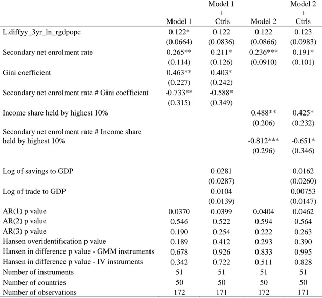
imperfections and political instability channels on economic growth. I use taxes on income, profits, and capital gains as a proxy for redistributive pressure, secondary school enrolment rates as a proxy of credit market imperfections and rule of law index as a proxy of political stability. In order to test the possible effects through these channel, income inequality, transmission channels and related interaction terms are added into the growth model. Following the SYS-GMM estimations on a panel dataset including 3-year averaged observations for 51 countries over a period from 1996 to 2015, the results show that there is negative interaction between income inequality and mentioned channels, even the direct impact income inequality is found as positive. Marginal effects of the related transmission channels are interpreted for different levels of income inequality.
Paper 3
Abstract
We investigate the impact of gender inequality in financial inclusion on income inequality, therefore making a three-fold contribution to the recent literature. First, using a micro-dataset covering 146,000 individuals in over 140 countries, we construct novel, synthetic indices of the intensity of financial inclusion at the individual level and country level. Second, we derive the distribution of individual financial access “scores” across countries to document a “Kuznets”-curve in financial inclusion. Third, cross-country regressions confirm that our measure of inequality in financial access in general, and financial access gaps between men and women in particular, is significantly related to income inequality, above and beyond other factors previously highlighted in the literature. Finally, our findings suggest that policies related to improving access to infrastructure, higher financial development and stronger institutions could significantly reduce involuntary exclusion.
Keywords: Democracy, economic growth, financial inclusion, financial development,
gender inequality, income inequality, panel data models, redistribution, sub-Saharan Africa
Contents
A SURVEY ON DIRECT AND INDIRECT EFFECTS OF INCOME INEQUALITY ON ECONOMIC GROWTH _________________________________________________7 INTRODUCTION__________________________________________________________8 LITERATURE REVIEW ___________________________________________________8 1. INCOME INEQUALITY, REDISTRIBUTION AND ECONOMIC GROWTH ___8
1.1. Income Inequality and Economic Growth ___________________________________8 1.2. Income Inequality and redistribution to the extent of the regime types ____________9 1.2.1. Democracy and Inequality ... 9 1.2.2. Democracy and Redistribution ... 10
2. INEQUALITY MEASURES ____________________________________________12 2.1. Graphical representation _______________________________________________12 2.1.1. Pen’s Parade ... 12 2.1.2. Lorenz Curve ... 13 2.2. Inequality measures ___________________________________________________14 2.2.1. Gini coefficient ... 14 2.2.2. Income shares... 14
3. INDIRECT IMPACT OF INCOME INEQUALITY ON ECONOMIC
GROWTH _______________________________________________________________14 4. METHODOLOGY ____________________________________________________15
4.1. Dynamic Panel Estimators ______________________________________________15 4.2. System GMM Estimator _______________________________________________17 4.3. Panel causality _______________________________________________________18
5. DISCUSSION _________________________________________________________18 REFERENCES ___________________________________________________________20
Appendix _________________________________________________________________26
NEGATIVE IMPACT OF INEQUALITY ON ECONOMIC GROWTH: TESTING TRANSMISSION CHANNELS _____________________________________________29 INTRODUCTION_________________________________________________________30 1. LITERATURE REVIEW _______________________________________________31
1.1. Political economy_____________________________________________________35 1.2. Credit market imperfections ____________________________________________35 1.3. Political instability ____________________________________________________37
2. METHODOLOGY ____________________________________________________39
2.1. The model __________________________________________________________39 2.2. Data _______________________________________________________________43 2.3. Estimations __________________________________________________________45
3. RESULTS ____________________________________________________________47
3.1. Political economy channel ______________________________________________47 3.2. Credit market imperfections channel ______________________________________51 3.3. Political and governance system channel __________________________________55
4. CONCLUSION _______________________________________________________58 REFERENCES ___________________________________________________________62
Appendix _________________________________________________________________68
INEQUALITY IN FINANCIAL INCLUSION, GENDER GAPS, AND INCOME
INEQUALITY ____________________________________________________________87 ABSTRACT ______________________________________________________________87 I. INTRODUCTION _______________________________________________________89 II. LITERATURE REVIEW ________________________________________________92
Finance and Inequality ______________________________________________________92 Gender gaps and inequality ___________________________________________________94 Gender gaps in financial inclusion _____________________________________________95 Putting the Pieces Together __________________________________________________96
III. DATA________________________________________________________________97
The Findex database ________________________________________________________97 Constructing Novel Indices of Financial Inclusion ________________________________98
IV. GENDER GAPS IN FINANCIAL INCLUSION AND INCOME INEQUALITY: EMPIRICAL STRATEGY ________________________________________________107
A. Specification___________________________________________________________107 B. Empirical Results _______________________________________________________108
Introduction and Summary
In the inequality and economic growth literature, both negative and positive effects of inequality are mentioned. Inequality which can undermine progress in health, education, causes investment reducing political and economic instability and undercuting the social consensus required to adjust in the face of shocks. Inequality is also said beneficial for growth, by fostering aggregate savings (Kuznets 1955, Kaldor 1956), by promoting high return projects (Rosenzweig and Binswanger 1993), by stimulating research and development (Foellmi and Zweimüller 2006). While observing the impact of income inequality, it should be considered possible side effects. Because, inequality may be harmful for the economic growth through socio-political instability, in other words, political system and social unrest, political economy and credit market imperfection channels. In other words, inequality may have indirect effects on economic growth by affecting these transmission channels.
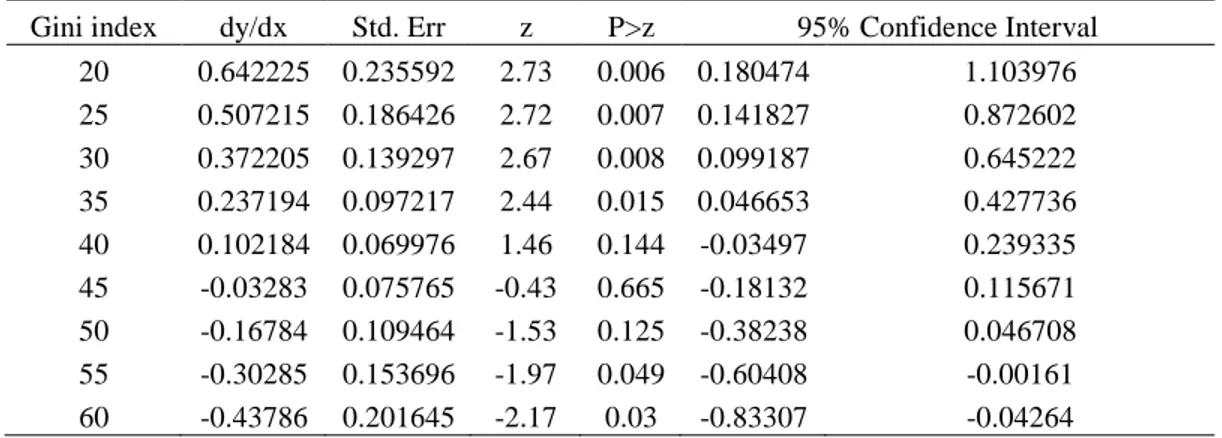
Related to the second paper, even though a negative direct effect was expected on economic growth, negative effects of income inequality only are justified through interactions with redistributive pressure, credit market imperfections and political instability channels, using selected variables as proxies for these channels. The results show that there is negative interaction between income inequality and mentioned channels, even the direct impact income inequality is found positive. Marginal effects of the related transmission channels are interpreted for different levels of income inequality. At the higher levels of income inequality, the impact of variables related to redistribution, political stability and human capital on economic growth vanishes and becomes sharper as inequality increases. In countries where income is distributed relatively equally, economic growth benefits from the positive impact of variables related to redistribution, political stability and human capital.
Third paper handles an independent problem arising from the unequal distribution of the financial access across population and across gender. inequality in financial access in general, and gender gaps in financial access, is significantly related to income inequality, controlling with other factors highlighted in the literature. We suggest policies which are related to improving access to infrastructure, higher financial development and stronger institutions could significantly reduce involuntary financial exclusion.
Chapter 1
A survey on direct and indirect effects of income inequality on economic
growth
Göksu Aslan
Abstract
In this paper, direct and indirect effects of the income inequality on economic growth is reviewed. First, the effects of income inequality and redistribution on economic growth are discussed to the extent of democracy. In the first section, its effects and in addition to the effects of redistribution and related studies are discussed to the extent of democracy. In the second section, main inequality measures are summarized. In the third section, indirect effects of income inequality through political economy, credit market imperfections and political instability channels are discussed in the light of existing studies. The fourth section reviews the model and dynamic panel estimators, especially system GMM. The last section concludes.
Keywords: Inequality, Economic Growth, Panel data models
Introduction
In this paper, the impact of income inequality on economic growth is reviewed. In the first section, its effects and in addition to the effects of redistribution and related studies are discussed to the extent of democracy. In the second section, main inequality measures are summarized. In the third section, indirect effects of income inequality through political economy, credit market imperfections and political instability channels are discussed in the light of existing studies. The fourth section reviews the model and dynamic panel estimators, especially system GMM. The last section concludes.
Literature Review
1. Income inequality, redistribution and economic growth
1.1. Income Inequality and Economic Growth
In the inequality and economic growth literature, both negative and positive effects of inequality are mentioned. Inequality which can undermine progress in health, education, causes investment reducing political and economic instability and undercuting the social consensus required to adjust in the face of shocks. Inequality is also said beneficial for growth, by fostering aggregate savings (Kuznets 1955, Kaldor 1956), by promoting high return projects (Rosenzweig and Binswanger 1993), by stimulating research and development (Foellmi and Zweimüller 2006).
Some inequality is integral to the effective functioning of a market economy and the incentives needed for investment and growth. As for the Okun’s (1975) big-trade-off hypothesis, a treatment for inequality as redistributive policies may be also worse for growth than disease itself by creating disincentives and inefficiencies. For societies, it is not possible to have both perfect equality and perfect efficiency. This hypothesis is not supported with empirical examples as the existence of societies such as Denmark, Luxembourg Sweden.
Inequality is harmful for growth by promoting expensive fiscal policies (Perotti 1993; Alessina and Rodrik 1994; Persson and Tabellini 1994); by inducing an inefficient state bureaucracy (Acemoglu et al. 2011), by hampering human capital formation (Bénabou 1996); or by undermining the legal system (Glaeser et al. 2003). The paper by Barro (2000) which shows a negative significant inequality impact in developing economies, applying simultaneous equation models and brings complex relationship between inequality and the fertility rate as the negative impact of inequality on economic growth is only significant when the fertility rate is omitted. Voitchovsky (2005), applying a SYS-GMM estimator shows a negative impact of the Gini coefficient. In connection with the fact that inequality and especially redistribution may have different effects on economic growth, in the following section these effects are discussed in the light of leading studies.
1.2. Income Inequality and redistribution to the extent of the regime types 1.2.1. Democracy and Inequality
The literature on the relationship between democracy and inequality has controversial findings. Sirowy and Inkeles (1990) find that the existing evidence suggest the level of political democracy as measured at one point of time tends not to be widely associated with lower levels of income inequality. They suggest that there may be evidence in favour of the relevance of the history of democracy for inequality. Muller (1988) finds a negative correlation between inequality and the numbers of years a country has been democratic. Simpson (1990), Burkhart (1997) and Gradstein and Justman (1999b) find a nonlinear reduced form relationship between democracy and inequality where at both low and high levels of democracy, inequality is lower, and higher at intermediate levels of democracy.
However, the impact of the history of democracy identified in the models that do not include fixed effects, it will capture the impact of these omitted fixed effects. This is a special case of the difficulty of identifying duration dependence and unobserved heterogeneity. (Acemoglu et.al, 2009)
Recent studies by Li et.al (1998), Rodrik (1999), and Scheve and Stasavage (2010) use better data and exploited the time as well as cross-sectional dimensions. Li et. Al (1998) find that an index of civil liberties is negatively correlated with inequality, such that greater civil liberties
are associated with lower inequality, using a pooled OLS. Rodrik (1999) finds a positive correlation between Freedom House of Polity III measure of democracy and both average real wages in manufacturing and the share of wages in national incomes, showing both in a cross-section and in a panel of countries using country fixed effects. Also, he finds an evidence that political competition and participation at large are important parts of the mechanisms via which democracy worked. Scheve and Stasavage (2009) use a long-run panel data from 1916 to 2000 for 13 OECD countries with country specific effects. They find a significant positive correlation between the universal suffrage dummy and the share of income accruing to people between the 90th and 99th percentiles of the income distribution divided by the share accruing to the people above the 99th percentile. Lee (2005) uses an unbalanced panel data with random effects, covering 64 countries for the period from 1970 to 1994. He finds a significant positive correlation between the size of government a measured by tax revenues as a percentage of GDP and democracy, suggesting that for large enough levels of government, democracy reduces inequality.
1.2.2. Democracy and Redistribution
Meltzer and Richard (1981) find that an expansion of democracy should lead to greater tax revenues and redistribution.
Gil et.al (2004) find no correlation between tax revenues and government spending measures and democracy, using a cross-sectional specification.
Aidt et.al (2006) and Aidt and Jensen (2009b) observe the impact of democratization measured by the proportion of adults who could vote in a cross national panel. Aidt et.al (2006) observe a cross sectional panel of 12 West European countries over the period 1830-1938. Aidt and Jensen (2009b) find positive effects of suffrage on government expenditure as percentage of GDP and also tax revenues as a percentage of GDP, using a cross national panel of 10 West European countries over the period 1860-1938.
Democracy is expected to change not only the amount of tax revenues, but also what taxes were used for. One might expect democracies to move towards more progressive taxation (Acemoglu et.al, 2015).
Aidt and Jensen (2009b) find that suffrage expansion lead to lower direct taxes and higher indirect taxes. Aidt and Jensen (2009a) find a nonlinear relationship between the introduction of an income tax and suffrage where an expansion of the franchise starting from very restrictive levels reduces the probability that an income tax will be introduced, but also that this probability increases at higher levels of the franchise. Scheve and Stasavage (2010, 2012) find no correlation between democracy and either tax progressivity or the rate of capital taxation, using a long-rung approach of the OECD countries. Lindert (1994) finds an impact of democracy on various types of social spending in a panel data over the period 1880-1930, stating that “There was so little social spending of any kind before the twentieth century mainly because political voice so restricted.”
Huber and Stephens (2012) find the story of democracy which is measured by the cumulative years a country has been democratic since 1945 is positively correlated with education spending, health spending, and social security and welfare spending, observing a panel dataset for Latin America between 1970-2007.
Kaufman and Segura-Ubiergo (2001) find that democracy which is measured by dichotomous measured introduced by Przeworski et.al (2000) is positively correlated with government expenditure on health and education. Brown and Hunter (1999) also show that democracies have greater social spending than autocracies, using democracy measured by Przeworski et.al (2000).
Persson and Tabellini (2003) find some evidence that democracy measured by the Gastil index and the Polity score, has positive effects on government expenditure and government revenues, and social security spending as percentage of GDP.
An additional focus of the democracy-redistribution literature is based on whether if female enfranchisement has an additional or differential impact on government taxation or spending. Results from Lindert (1994) showing that financial enfranchisement has an independent impact on social spending are consistent with Aidt and Dallal (2008) for a later period. Lott and Kenny (1999) find that the expansion of women’s voting rights in the United States between 1870 and 1940 is associated with increases in per capita government revenues and expenditures. Miller
(2008) shows that female suffrage increases health spending and let to significant falls in infant mortality.
Aidt and Jensen (2013) provides an identification strategy for the endogeneity of the democracy. They argue that revolutionary threat measured by revolutionary events in other countries is a viable instrument for democracy in a panel of West European countries, building on the theoretical ideas of Acemoglu and Robinson (2000, 2006) and Aidt and Jensen (2011). They find that democracy measured by the extent of suffrage has a robust positive effect on government spending.
Acemoglu et.al (2015) explain that the expectation in the literature has been that democracy should increase redistribution and reduce inequality, and why this expectation may not be borne out in the data because democracy may be captured or constrained, because democracy may cater to the wishes of the middle class, or because democracy may be simultaneously open up new economic opportunities to the previously excluded, contributing to economy inequality. They find that democratization increases government taxation and revenue as fractions of GDP, confirming the (basic) (prediction) (of the) standard Meltzer-Richard model. They do not find a robust evidence that democracy reduces inequality.
2. Inequality Measures
Measuring inequality is to find a scalar or distributional representation of the interpersonal differences in income within a given population. There are several ways to represent inequality in graphical form such as Pen’s Parade, frequency distribution, Lorenz Curve and logarithmic transformation. In the following sections, Pen’s Parade, Lorenz Curve, Gini coefficient and income shares are explained. The calculation of Gini coefficient revised and additionally covariance based calculation is mentioned in Appendix.
2.1. Graphical representation
2.1.1. Pen’s Parade
Pen's Parade or The Income Parade is a concept described in a 1971 book published by Dutch economist Jan Pen describing income distribution. The parade is defined as a succession of every person in the economy, with their height proportional to their income, and ordered from
lowest to greatest. People with average income would be of average height, and so the spectator. The Pen's description of what the spectator would see is a parade of dwarves, and then some unbelievable giants at the very end. (Crook, 2006)
The parade is used by economists as a graphical representation of income inequality because it’s a form of Quantile function and it is considered useful when comparing two different areas or periods. (Haughton and Khandker, 2009)
2.1.2. Lorenz Curve
The Lorenz Curve is a tool used to represent income distributions as proposed by Lorenz (1905). It relates the cumulative proportion of income to the cumulative proportion of individuals.
The Lorenz Curve is obtained as follows:
The x-axis records the cumulative proportion of population ranked by income level. It ranges between 0 and 1.
The y-axis records the cumulative proportion of income for a given proportion of population, i.e. the income share calculated by taking the cumulated income of a given share of the population, divided by the total income Y.
Figure 1. Lorenz Curve
2.2. Inequality measures
2.2.1. Gini coefficient
The most widely used single measure of inequality is the Gini coefficient which was developed by Italian statistician Corrado Gini (1884-1965). It is based on the Lorenz curve, a cumulative frequency curve that compares the distribution of a specific variable with the uniform distribution that represents equality. To construct the Gini coefficient, graph the cumulative percentage of households (from poor to rich) on the horizontal axis and the cumulative percentage of income on the vertical axis. The diagonal line represents perfect equality. The Gini coefficient is defined as A/(A + B), where A and B are the areas shown in the Figure 1. If A= 0, the Gini coefficient becomes 0, which means perfect equality, whereas if B = 0, the Gini coefficient becomes 1, which means complete inequality. Gini coefficient of zero represents a distribution where the Lorenz curve is just the ‘Line of Equality’ and incomes are perfectly equally distributed – a value of 1 means maximal inequality. (Haughton & Khandker, 2009)
Let 𝑥𝑖 is a point on the x-axis, and 𝑦𝑖 is a point on the y-axis. Then
𝐺𝑖𝑛𝑖 = 1 − ∑𝑁𝑖=1(𝑥𝑖− 𝑥𝑖−1)(𝑦𝑖 + 𝑦𝑖−1) (1)
When there are N equal intervals on the x-axis, equation simplifies to
𝐺𝑖𝑛𝑖 = 1 −1
𝑁∑ (𝑦𝑖+ 𝑦𝑖−1)
𝑁
𝑖=1 (2)
2.2.2. Income shares
Percentage share of income or consumption is the share that accrues to subgroups of population indicated by deciles, quintiles or interested percentage of population. Income share held by top 1, 10, 20 percent of the population, or similarly also income share held by bottom 10, 20, 40 percent of the population are widely used measures.
3. Indirect impact of income inequality on economic growth
While observing the effects of income inequality, the indirect effects of income inequality through various transmission channels should be analysed as well as its direct effects. Because,
inequality may be harmful for the economic growth through socio-political instability, in other words, political system and social unrest, political economy and credit market imperfection channels. In other words, inequality may have indirect effects on economic growth by affecting these transmission channels. The main focus of the third chapter is to test negative impact of income inequality, through these channels. The impact of these channels and their interactions with income inequality are explained deeper in the third chapter.
4. Methodology
4.1. Dynamic Panel Estimators
Dynamic relationships are characterized by the presence of a lagged dependent variable among the regressors as below:
𝑦𝑖𝑡 = 𝛿𝑦𝑖,𝑡−1+ 𝑥𝑖𝑡′𝛽 + 𝑢𝑖𝑡 𝑖 = 1, … , 𝑁; 𝑡 = 1, … , 𝑇 (3)
where δ is a scalar, 𝑥𝑖𝑡′ is 1 × K and β is K × 1, the 𝑢
𝑖𝑡 is assumed follow a one-way error
component model
𝑢𝑖𝑡 = 𝜇𝑖+ 𝑣𝑖𝑡 (4)
where 𝜇𝑖~𝐼𝐼𝐷(0, 𝜎𝜇2) and 𝜇
𝑖~𝐼𝐼𝐷(0, 𝜎𝜇2) independent of each other and among themselves.
The dynamic panel data regression described in (3) and (4) is characterized by two sources of persistence over time. Autocorrelation due to the presence of a lagged dependent variable among the regressors and individual effects characterizing the heterogeneity among the individuals.
Since 𝑦𝑖𝑡 is a function of 𝜇𝑖, 𝑦𝑖,𝑡−1 is also a function of 𝜇𝑖. Therefore, 𝑦𝑖,𝑡−1 is correlated with the error term. This causes the OLS estimator biased and inconsistent even if 𝑣𝑖𝑡 are not serially correlated. For the fixed effects (FE) estimator, the Within transformation wipes out the 𝜇𝑖, but
(𝑦𝑖,𝑡−1− 𝑦̅𝑖.−1) where 𝑦̅𝑖.−1= ∑ 𝑦𝑇2 𝑖,𝑡−1/(𝑇 − 1) will still be correlated with 𝑣𝑖𝑡 − 𝑣̅𝑖.) even
if the 𝑣𝑖𝑡 are not serially correlated. This is because 𝑦𝑖,𝑡−1 is correlated with 𝑣̅𝑖. by construction. The latter average contains 𝑣𝑖,𝑡−1 which is obviously correlated with 𝑦𝑖,𝑡−1. In fact, the Within estimator will be biased of 𝑂(1/𝑇) and its consistency will depend upon 𝑇 being large. More
recently, Kiviet (1995) derives an approximation for the bias of the Within estimator in a dynamic panel data model with serially uncorrelated disturbances and strongly exogenous regressors. Kiviet (1995) proposed a corrected Within estimator that subtracts a consistent estimator of this bias from the original Within estimator. Therefore, for the typical labour panel where N is large and T is fixed, the Within estimator is biased and inconsistent. It is worth emphasizing that only if 𝑇 → ∞ will the Within estimator of δ and β be consistent for the dynamic error component model. For macro panels, studying for example long-run growth, e.g. Islam (1995) the data covers a large number of countries N over a moderate size T. In this case, T is not very small relative to N. Hence, some researchers may still favour the within estimator arguing that its bias may not be large. Judson and Owen (1999) performed some Monte Carlo experiments for N = 20 or 100 and T = 5, 10, 20 and 30 and found that the bias in the Within estimator can be sizeable, even when T = 30. This bias increases with δ and decreases with T. But even for T = 30, this bias could be as much as 20% of the true value of the coefficient of interest. The random effects GLS estimator is also biased in a dynamic panel data model. In order to apply GLS, quasi-demeaning is performed and (𝑦𝑖,𝑡−1− 𝜃𝑦̅𝑖.−1) will be correlated with (𝑢𝑖,𝑡−1− 𝜃𝑢̅𝑖.−1). An alternative transformation that wipes out the individual effects is the first difference (FD) transformation. In this case, correlation between the predetermined explanatory variables and the remainder error is easier to handle. In fact, Anderson and Hsiao (1981) suggested first differencing the model to get rid of the 𝜇𝑖 and then using ∆𝑦𝑖,𝑡−2 = (𝑦𝑖,𝑡−2− 𝑦𝑖,𝑡−3) or 𝑦𝑖,𝑡−2 as an instrument for ∆𝑦𝑖,𝑡−1 = (𝑦𝑖,𝑡−1− 𝑦𝑖,𝑡−2). These instruments will not be correlated with ∆𝑣𝑖𝑡 = (𝑣𝑖,𝑡− 𝑣𝑖,𝑡−1), as long as the 𝑣𝑖𝑡 themselves are not serially correlated. This instrumental variable (IV) estimation method leads to consistent but not necessarily efficient estimates of the parameters in the model because it does not make use of all the available moment conditions and it does not take into account the differenced structure on the residual disturbances (∆𝑣𝑖𝑡). Arellano (1989) finds that for simple dynamic error components models, the estimator that uses differences ∆𝑦𝑖,𝑡−2 rather than levels
𝑦𝑖,𝑡−2for instruments has a singularity point and very large variances over a significant range
of parameter values. In contrast, the estimator that uses instruments in levels, i.e. 𝑦𝑖,𝑡−2, has no singularities and much smaller variances and is therefore recommended. Arellano and Bond (1991) proposed a generalized method of moments (GMM) procedure that is more efficient than the Anderson and Hsiao (1982) estimator, while Ahn and Schmidt (1995) derived
additional nonlinear moment restrictions not exploited by the Arellano and Bond (1991) GMM estimator. This literature is generalized and extended by Arellano and Bover (1995) and Blundell & Bond (1998) to mention a few. In addition, an alternative method of estimation of the dynamic panel data model which is proposed by Keane and Runkle (1992) is based on the forward filtering idea in time-series analysis. (Baltagi, 2005)
4.2. System GMM Estimator
Since the right-hand-side variables are typically endogenous and measured with error, and there are omitted variables, estimating growth regressions becomes problematic. In the presence of omitted variables, least squares parameter estimates are biased (Bond et.al, 2001). Applying OLS creates the problem that 𝑌𝑖,𝑡−1 is correlated with the fixed effects in the error term, which causes dynamic panel bias (Nickell, 1981).
The difference and system GMM estimators are designed for dynamic panel analysis where current realizations of the dependent variable influenced by past ones in the cases where large N, small T. There may be arbitrarily distributed fixed individual effects. This argues against cross-section regressions, which must essentially assume fixed effects away, and in favour of a panel setup, where variation over time can be used to identify parameters. The DIFF-GMM and SYS-GMM estimator assume that some regressors may be endogenous; the idiosyncratic disturbances (those apart from the fixed effects) may have individual specific patterns of heteroskedasticity and serial correlation; the idiosyncratic disturbances are uncorrelated across individuals. Some regressors can be predetermined but not strictly exogenous. Finally, because the estimators are designed for general use, they do not assume that good instruments are available outside the immediate dataset. In effect, it is assumed that the only available instruments are “internal” - based on lags of the instrumented variables. However, the estimators do allow inclusion of external instruments (Roodman, 2009).
Comparing to DIFF-GMM estimator, the SYS-GMM estimator has many advantages as in variables which are random-walk or close to be random-walk (Baum, 2006). By using DIFF-GMM, differencing variables within groups will remove any variable that is constant. SYS-GMM produces more efficient and precise estimates compared to DIFF-SYS-GMM, by improving precision and reducing the finite sample bias (Baltagi, 2008). While working unbalanced panel as in our panel dataset, DIFF-GMM approach is weak in filling gaps (Roodman, 2006, p.20).
The SYS-GMM estimator is unbiased and most efficient if there are endogenous predetermined regressors.
By construction, the residuals of the differenced equation should possess serial correlation, but if the assumption of serial independence in the original errors is warranted, the differenced residuals should not exhibit significant AR(2) behaviour. If a significant AR(2) statistic is encountered, the second lags of endogenous variables will not be appropriate instruments for their current values ( Baum, 2013).
4.3. Panel causality
Panel VAR models have been widely used in multiple applications across fields, with the introduction of VAR in panel data settings (Holtz-Eakin, Newey and Rosen, 1988).
Panel VAR Granger causality procedure is developed by Abrigo and Love (2015) following panel VAR procedure developed by Love and Zicchino (2006).Abrigo and Love (2015) giving an overview of panel VAR model selection, estimation and inference in a generalized method of moments (GMM) framework, provide a package of Stata programs, with additional functionality, including sub-routines to implement Granger (1969) causality tests. 1
5. Discussion
Income inequality, in its different forms, such as Gini index or income shares of deciles of population, may harmful for economic growth. Policies reducing inequality, such as higher tax policies, may be also destructive for the economic growth. These effects could differ to the extent of democracy. In democracies, governments tend to redistribute significantly more. Additionally, income inequality may have indirect effects through reducing non-obligatory school enrolment rates related to the fact that poor people cannot invest in education, since they do not have access to credit. Finally, income inequality may have indirect effects through creating instable political and social environment.
While observing the impact of income inequality, it should be considered possible side effects. Because, inequality may be harmful for the economic growth through socio-political
instability, in other words, political system and social unrest, political economy and credit market imperfection channels. In other words, inequality may have indirect effects on economic growth by affecting these transmission channels.
As regard as empirical studies, analysing the impact of inequality contains the endogeneity problem of the right-hand side variables. It should be paid attention in using right and exactly identifying instrumental variables. One problem arising from the panel data with large N is to have small T for some of the cross sections in the dataset. The difference and system GMM estimators are designed for dynamic panel analysis where current realizations of the dependent variable influenced by past ones in the cases where large N, small T. Other problem is to have endogeneity while observing the effects of inequality on economic growth, because of the unavailability of time-variant exogenous regressors, following the difference and system GMM estimators would be appropriate approach if the instruments are correctly used.
As regard as several income inequality measures, Gini index is most widely used among them. Income shares of the deciles or quantiles of the population are also highly informative on how income distributed within population.
Another important issue is that how income inequality change before and after taxes and transfers. If inequality after taxes and transfer, in other words net inequality, is quite lower than inequality before taxes and transfer; this means that redistributive policies are implemented in the favour of the poor. Inequality effects on economic growth may be handled as before and after taxes, or with the implementation of the effects of redistributive policies. As mentioned above, these redistributive policies may differ to the extent of democracy levels of countries. As is the case that income inequality may have direct impact on economic growth, it may affect the marginal impact of several important variables related to redistributive policies, human capital, or political stability. These effects may arise undermining progress in health, education, causes investment reducing political and economic instability and undercutting the social consensus required to adjust in the face of shocks. These negative effects should be considered in the context of unequal opportunities arising from unequal distributed income among the population.
References
Abrigo, Michael and Inessa Love (2016). “Estimation of Panel Vector Autoregression in Stata: a Package of Programs”. The Stata Journal, 16(3): 1-27.
Acemoglu, D., & Robinson, J. (2000). Why did the west extend the franchise? Q. J. Econ. 115, 1167–1199.
Acemoglu, D., & Robinson, J. (2006). Economic Origins of Dictatorship and Democracy. New York, NY: Cambridge University Press.
Acemoglu, D., Johnson, S., Robinson, J., & Yared, P. (2009). Reevaluating the modernization hypothesis. J. Monet. Econ. 56, 1043-1058.
Acemoglu, D., Naidu, S., Restrepo, P., & Robinson, J. (2015). Democracy, redistribution and inequality. In A. B. Atkinson, Handbook of Income Distribution, vol 2B. Chapter 21 (pp. 1885-1996). Amsterdam: Elsevier.
Acemoglu, D., Ticchi, D., & Vindigni, A. (2011). Emergence and persistence of inefficient states. J. Eur. Econ. Assoc., 9 (2), 177–208.
Ahn, S., & Schmidt, P. (1995). Efficient estimation of models for dynamic panel data. Journal of Econometrics, 68, 5–27.
Aidt, T., & Dallal, B. (2008). Female voting power: the contribution of women’s suffrage to the growth of social spending in Western Europe (1869–1960). Public Choice 134 (3–4), 391–417.
Aidt, T., & Jensen, P. (2009a). The taxman tools Up: an event history study of the
introduction of the personal income Tax in western Europe, 1815–1941. J. Public Econ. 93, 160–175.
Aidt, T., & Jensen, P. (2009b). Tax structure, size of government, and the extension of the voting franchise in western Europe, 1860–1938. Int. Tax Public Fin. 16 (3), 362–394. Aidt, T., & Jensen, P. (2011). Workers of the World Unite! Franchise Extensions and the
Threat of Revolution in Europe. Cambridge Working Papers in Economics 1102, Faculty of Economics, University of Cambridge, pp. 1820-1938.
Aidt, T., & Jensen, P. (2013). Democratization and the size of government: evidence from the long 19th. http://ideas.repec.org/p/ces/ceswps/_4132.html.
Aidt, T., & Jensen, P. (2013). Democratization and the size of government: evidence from the long 19th century. Public Choice 157 (3-4), 511-542.
Aidt, T., & Jensen, P. (n.d.). Workers of the World Unite! Franchise Extensions and the Threat of Revolution in Europe, 1820–1938. Cambridge Working Papers in Economics 1102, Faculty of Economics. 2011: University of Cambridge. Aidt, T., Dutta, J., & Loukoianova, E. (2006). Democracy comes to Europe: franchise
expansion and fiscal 1830–1938. Eur. Econ. Rev. 50 (2), 249–283.
Alesina, A., & Perotti, R. (1994). Income Distribution, Political Instability and Investment. 1994-95 Discussion Paper Series No. 751.
Alesina, A., & Rodrik, D. (1994). Distributive Politics and Economic Growth. Quarterly Journal of Economics, 109, 465-490.
Alesina, A., & Tabellini, G. (1989). External Debt, Capital Flight and Political Risk. Journal of International Economics, 27, 199-220.
Alesina, A., Ozler, S., Roubini, N., & Swagel, P. (1996). Political Instability and Economic Growth. Journal of Economic Growth, 1(2), 189-211.
Anderson, T., & Hsiao, C. (1981). Estimation of dynamic models with error components. Journal of the American Statistical Association, 76, 598–606.
Arellano, M. (1989). A note on the Anderson–Hsiao estimator for panel data. Economics Letters, 31, 337–341.
Arellano, M., & Bond, S. (1991). Some tests of specification for panel data: Monte Carlo evidence and an application to employment equations. Review of Economic Studies, 58, 277–297.
Arellano, M., & Bover, O. (1995). Another look at the instrumental variables estimation of errorcomponent models. Journal of Econometrics, 68, 29–51.
Baltagi, B. (2005). Econometric Analysis of Panel Data (Third ed.). John Wiley & Sons, Ltd. Barro, R. (1989). A Cross-Country Study of Growth, Saving and Government. NBER
Working Paper No. 2855.
Barro, R. (1991). Economic Growth in a Cross Section of Countries. The Quarterly Journal of Economics, Vol. 106, No.2, 407-443.
Barro, R. (2000). Inequality and Growth in a Panel of Countries. Journal of Economic Growth, 5, 5-32.
Baum, C. (2006). An Introduction to Modern Econometrics using Stata. Stata Press books, StataCorp LP, number imeus September.
Baum, C. (2013). Implementing new econometric tools in Stata. Mexican Stata Users' Group Meetings. Stata Users Group.
Baum, C., & Schaffer, M. (2003). Instrumental variables and GMM: Estimation and testing. The Stata Journal. 3(1), 1-31.
Baum, C., Schaffer, M., & Stillman, S. (2007). Enhanced routines for instrumental
variables/generalized method of moments estimation and testing. The Stata Journal, 7(4), 465-506.
Bénabou, R. (1996). Inequality and Growth. CEPR Discussion Papers 1450, C.E.P.R. Discussion Papers.
Bénabou, R. (n.d.). Equity and Efficiency in Human Capital Investment: The Local Connection. Review of Economic Studies, 63(2), 237-264.
Berg, A. G., & Ostry, J. D. (2011). Inequality and Unsustainable Growth: Two Sides of the Same Coin? . IMF (Ed.), IMF Staff Discussion Note.
Berg, A., & Sachs, J. (1988). The Debt Crisis: Structural Explanations of Country Performance . Journal of Development Economics, Vol. 29, No. 3, 271–306.
Blundell, R., & Bond, S. (1998). Initial conditions and moment restrictions in dynamic panel data models. Journal of Econometrics, 87, 115-143.
Bond, S. (2002). Dynamic panel data models: a guide to micro data methods and practice. Portuguese Economic Journal, 141–162. doi:0.1007/s10258-002-0009-9
Bond, S., Anke, H., & Temple, J. (2001). GMM Estimation of Empirical Growth Models. CEPR Discussion Papers, 3048.
Brown, D., & Hunter, W. (1999). Democracy and social spending in Latin America, 1980–92 . Am. Polit Sci. Rev. 93 (4), 779–790.
Burkhart, R. (1997). Comparative democracy and income distribution: shape and direction of the causal arrow. J. Polit. 59 (1), pp. 148-164.
Crook, C. (2006, September). The Height of Inequality. The Atlantic. Retrieved 28 May 2015.
Foellmi, R., & Zweilmueller, J. (2006). Structural Change and the Kaldor Facts of Economic Growth . 2006 Meeting Papers 342, Society for Economic Dynamics.
Galor, O., & Zeira, J. (1993). Income Distribution and Macroeconomics. Review of Economic Studies, 60, 35-52.
Gil, R., Mulligan, C., & Sala-i-Martin, X. (2004). Do democracies have different public policies than nondemocracies? J. Econ. Perspect. 18, 51–74.
Glaeser, E. (2003). Introduction to "The Governance of Not-for-Profit Organizations". NBER Chapters, pp. 1-44.
Gradstein, M., & Justman, M. (1999b). The democratization of political elites and the decline in inequality in modern economic growth. In E. Breizes, & P. (. Temin, Elites,
Minorities and Economic Growth. Amsterdam: Elsevier.
Grossman, H. (1991). A General Equilibrium Model of Insurrections. American Economic Review, 81(4), 912-921.
Haughton, J., & Khandker, S. (2009). Handbook on Poverty and Inequality. World Bank Publications, The World Bank, number 11985.
Huber, E., & Stephens, J. (2012). Democracy and the Left: Social Policy and Inequality in Latin America. University of Chicago Press, Chicago, IL.
Islam, N. (1995). Growth Empirics: A Panel Data Approach. The Quarterly Journal of Economics, 110(4), 1127-70.
Judson, R., & Owen, A. (1999). Estimating dynamic panel data models: A guide for macroeconomists. Economics Letters, 65, 9-15.
Kaldor, N. (1956). Alternative Theories of Distribution. Review of Economic Studies, 23, 83-100.
Kaufman, R., & Segura-Ubiergo, A. (2001). Globalization, domestic politics, and social spending in Latin America: a time-series cross-section analysis, 1973–97. World Polit. 53 (4), 553–587.
Keane, M., & Runkle, D. (1992). On the estimation of panel-data models with serial correlation when instruments are not strictly exogenous. Journal of Business and Economic Statistics, 10, 1-9.
Kiviet, J. (1995). On bias, inconsistency and efficiency of various estimators in dynamic panel data models. Journal of Econometrics, 68, 53–78.
Kormendi, R., & Meguire, P. (1985). Macroeconomic Determinants of Growth: Cross-Country evidence. Journal of Monetary Economics, 141-163.
Kuznets, S. (1955). Economic Growth and Income Inequality. American Economic Review 65, 1-28.
Lee, C.-S. (2005). Income inequality, democracy, and public sector size. Am. Sociol. Rev. 70 (1), 158–181.
Li, H., Squire, L., & Zou, H.-f. (1998). Explaining international and intertemporal variations in income inequality. Econ. J. 108 (1), 26-43.
Lindert, P. (1994). The rise of social spending, 1880–1930. Explor. Econ. Hist. 31 (1), 1-37. Londregan, J., & Poole, K. (1990, January). Poverty, The Coup Trap and The Seizure of
Executive Power. World Politics.
Lorenz, M. (1905). Methods of Measuring the Concentration of Wealth. Journal of the American Statistical Association (new series), 70, 209-217.
Lott Jr., J., & Kenny, L. (1999). How dramatically did women’s suffrage change the size and scope of government? J. Polit. Econ. 107 (6), 1163–1198.
Loury, G. (1981). Intergenerational Transfers and the Distribution of Earnings. Econometrica , Vol. 49, No. 4, 843-867.
Love, I. and L. Zicchino (2006). Financial development and dynamic investment behavior: Evidence from panel VAR. The Quarterly Review of Economics and Finance, 46(2), 190-210.
Meltzer, A., & Richard, S. (1981). A rational theory of the size of government. J. Polit. Econ. 89, 914-927.
Miller, G. (2008). Women’s suffrage, political responsiveness, and child survival in American history. Q. J. Econ. 123 (3), 1287–1327.
Muller, E. (1988). Democracy, economic development, and income inequality. Am. Sociol. Rev. 53 (1), 50-68.
Nickell, S. (1981, November). Biases in Dynamic Models with Fixed Effects. Econometrica. Econometrica, Vol. 49, No. 6 (, 49(6), 1417-1426.
Okun, A. (1975). Equality and Efficiency: the Big Trade-Off. Brookings Institution Press. Ortiz-Ospina, E., & Roser, M. (2016). Income Inequality. Retrieved from
OurWorldInData.org: ourworldindata.org/income-inequality
Perotti, R. (1993, September). Political Equilibrium, Income Distribution, and Growth. Review of Economic Studies, 60(4), 755-776.
Persson, T., & Tabellini, G. (2003). The Economic Effects of Constitutions. MIT Press, Cambridge.
Przeworski, A., Alvarez, M., Cheibub, J., & Limongi, F. (2000). Democracy and
Development: Political Institutions and Material Well-being in the World, 1950– 1990. New York, NY: Cambridge University Press.
Rodrik, D. (1999). Democracies pay higher wages. . Q. J. Econ. 114, 707–738.
Roodman, D. (2006). How to Do xtabond2: An Introduction to "Difference" and "System" GMM in Stata. Working Papers 103, Center for Global Development.
Roodman, D. (2009). How to do xtabond2: An introduction to difference and system GMM. The Stata Journal,, 9(1), 86-136.
Rosenzweig, M., & Binswanger, H. (1993). Wealth, Weather Risk and the Composition and Profitability of Agricultural Investments. Economic Journal 103(416), 56-78.
Scheve, K., & Stasavage, D. (2009). Institutions, Partisanship, and Inequality in the Long Run. World Polit. 61, 215–253.
Scheve, K., & Stasavage, D. (2010). The conscription of wealth: mass warfare and the demand for progressive taxation. Inter. Organ. 64, 529–561.
Scheve, K., & Stasavage, D. (2012). Democracy, war, and wealth: lessons from two centuries of inheritance taxation. Am. Polit. Sci. Rev. 106 (1), 82–102.
Simpson, M. (1990). Political rights and income inequality: a cross-national test. Am. Sociol. Rev. 55 (5), 682-693.
Sirowy, L., & Inkeles, A. (1990). The effects of democracy on economic growth and inequality: a review. Stud. Comput. Inter. Develop. 25, pp. 126-57.
Stiglitz, J. (2012). The Price of Inequality: How Today's Divided Society Endangers Our Future. W. W. Norton & Company.
Voitchovsky, S. (2005). Does the Profile of Income Inequality Matter for Economic Growth? Journal of Economic Growth, 10(3), 273-296.
Appendix
Box 1. Covariance based calculation of Gini coefficient
Covariance-based Gini coefficient as mentioned by Yitzhaki (1998):
𝐺𝐼𝑁𝐼(𝑋) = −2𝐶𝑜𝑣 ( 𝑋
𝜇(𝑋), (1 − 𝐹(𝑋)))
Where X is a random variable of interest with mean 𝜇(𝑋) and 𝐹(𝑋) is its cumulative distribution function. The Concentration coefficient measures the association between two random variables and can be expressed as
𝐶𝑂𝑁𝐶(𝑋, 𝑌) = −2𝐶𝑜𝑣 ( 𝑋
𝜇(𝑋), (1 − 𝐺(𝑌)))
Where 𝐺(𝑌) is the cumulative distribution function of Y. 𝐶𝑂𝑁𝐶(𝑋, 𝑌) reflects how much X concentrated on observations with high ranks in Y.
A single-parameter generalization of the Gini coefficient has been proposed by Donaldson & Weymark (1980, 1983) and Yitzhaki (1983). The generalized Gini coefficient (S-Gini, or extended Gini coefficient) can also be expressed as a covariance:
𝐺𝐼𝑁𝐼(𝑋; 𝑣) = −𝑣𝐶𝑜𝑣 ( 𝑋
𝜇(𝑋), (1 − 𝐹(𝑋))
𝑣−1)
Where 𝑣 is a parameter tuning the degree of ‘aversion to inequality’. The standard Gini correspongs to 𝑣=2 The fractional ranks are calculated as following
Consider a sample of N observations on a variable Y with associated sample weights: {(𝑦𝑖, 𝑤𝑖)}𝑖=1𝑁 . Lek K be
the number of distinct values observerd on Y, denoted 𝑦1∗< 𝑦2∗< ⋯ < 𝑦𝑘∗, and denote by 𝜋𝑘∗ the corresponding
weighted sample proportions:
𝜋𝑘∗ =
∑𝑁𝑖=1𝑤𝑖1(𝑦𝑖= 𝑦𝑘∗)
∑𝑁𝑖=1𝑤𝑖
(1(condition) is equal to 1 if condition is true and 0 otherwise). The fractional rank attached to each 𝑦𝑘∗ is given
by
𝐹𝑘∗= ∑ 𝜋𝑗∗+ 0.5𝜋𝑘∗
𝑘−1
𝑗=0
where 𝜋0∗= 0 (Lerman & Yitzhaki, 1989, Chotikapanich & Griffiths, 2001). Each observation in the sample is
then associated with the fractional rank
𝐹𝑘∗= ∑ 𝐹𝑘∗1(𝑦𝑖= 𝑦𝑘∗)
𝐾
𝑘=1
This procedure ensures that tied observations are associated with identical fractional ranks and that the sample
mean of the fractional ranks is equal to 0.5. {(𝐹𝑖, 𝑦𝑖, 𝑤𝑖)}𝑖=1𝑁 can then be plugged in a standard sample
covariance formula. This makes the resulting Gini coefficient estimate independent on the sample/population size.
Box2. Panel VAR specification
Abrigo and Love (2015) consider a 𝑘-variate homogeneous panel VAR of order 𝑝 with panel-specific fixed effects represented by the following system of linear equations:
𝒀𝒊𝒕= 𝒀𝒊𝒕−𝟏𝑨𝟏+ 𝒀𝒊𝒕−𝟐𝑨𝟐+ ⋯ + 𝒀𝒊𝒕−𝒑+𝟏𝑨𝒑−𝟏+ 𝒀𝒊𝒕−𝒑𝑨𝒑+ 𝑿𝒊𝒕𝑩 + 𝒖𝒊+ 𝒆𝒊𝒕
𝑖 ∈ {1,2, … , 𝑁}, 𝑡 ∈ {1,2, … , 𝑇𝑖}
(1)
where 𝒀𝒊𝒕 is a (1𝑥𝑘) vector of dependent variables; 𝑿𝒊𝒕 is a (1𝑥𝑙) vector of exogenous covariates; 𝒖𝒊 and 𝒆𝒊𝒕
are (1𝑥𝑘) vectors of dependent variable-specific panel fixed-effects and idiosyncratic errors, respectively. The
(𝑘𝑥𝑘) matrices 𝑨𝟏, 𝑨𝟐, … , 𝑨𝒑−𝟏, 𝑨𝒑 and the (𝑙𝑥𝑘) matrix 𝑩 are parameters to be estimated. We assume that
the innovations have the following characteristics: 𝑬[𝒆𝒊𝒕] = 𝟎, 𝑬[𝒆𝒊𝒕′𝒆𝒊𝒕] = 𝚺 and 𝑬[𝒆𝒊𝒕′𝒆𝒊𝒔] = 𝟎 for all 𝑡 > 𝑠.
The parameters above may be estimated jointly with the fixed effects or, alternatively, independently of the fixed effects after some transformation, using equation-by-equation ordinary least squares (OLS). With the presence of lagged dependent variables in the right-hand side of the system of equations, however, estimates
would be biased even with large 𝑁 (Nickell, 1981). Although the bias approaches zero as 𝑇 gets larger,
simulations by Judson and Owen (1999) find significant bias even when 𝑇 = 30.
GMM Framework
Various estimators based on GMM have been proposed to calculate consistent estimates of the above equation, especially in fixed 𝑇 and large 𝑁 settings. With our assumption that errors are serially uncorrelated, the first-difference transformation may be consistently estimated equation-by-equation by instrumenting lagged
differences with differences and levels of 𝒀𝒊𝒕 from earlier periods as proposed by Anderson and Hsiao (1982).
This estimator, however, poses some problems. The first-difference transformation magnifies the gap in
unbalanced panels. For instance, if some 𝒀𝒊𝒕−𝟏 are not available, then the first-differences at time 𝑡 and 𝑡 − 1
are likewise missing. Also, the necessary time periods each panel is observed gets larger with the lag order of
the panel VAR. As an example, for a second-order panel VAR, instruments in levels require that 𝑇𝑖≥ 5
Box2. Panel VAR specification contd’
Arellano and Bover (1995) proposed forward orthogonal deviation as an alternative transformation, which does not share the weaknesses of the first-difference transformation. Instead of using deviations from past realizations, it subtracts the average of all available future observations, thereby minimizing data loss. Since past realizations are not included in this transformation, they remain valid instruments. Potentially, only the
most recent observation is not used in estimation. In a second-order panel VAR, for instance, only 𝑇𝑖≥ 4
realizations are necessary to have instruments in levels. Improving efficiency by including a longer set of lags as instruments will reduce observations especially with unbalanced panels or with missing observations, in general. As a remedy, Holtz-Eakin, Newey and Rosen (1988) proposed creating instruments using observed realizations, with missing observations substituted with zero, based on the standard assumption that the instrument list is uncorrelated with the errors.
While equation-by-equation GMM estimation yields consistent estimates of panel VAR, estimating the model as a system of equations may result in efficiency gains (Holtz-Eakin, Newey and Rosen, 1988). Suppose the
common set of 𝐿 ≥ 𝑘𝑝 + 𝑙 instruments is given by the row vector 𝒁𝒊𝒕, where 𝑿𝒊𝒕∈ 𝒁𝒊𝒕, and equations are
indexed by a number in superscript. Consider the following transformed panel VAR model based on equation (1) but represented in a more compact form:
𝒀𝒊𝒕∗ = 𝒀̅̅̅̅𝑨 + 𝒆𝒊𝒕∗ 𝒊𝒕∗ 𝒀𝒊𝒕∗ = [𝒚𝒊𝒕𝟏∗ 𝒚𝟐∗𝒊𝒕 … 𝒚𝒊𝒕𝒌−𝟏∗ 𝒚𝒊𝒕𝒌∗ ] 𝒀𝒊𝒕∗ ̅̅̅̅ = [𝒀𝒊𝒕−𝟏∗ 𝒀𝒊𝒕−𝟐∗ … 𝒀𝒊𝒕−𝒑+𝟏∗ 𝒀𝒊𝒕−𝒑∗ 𝑿𝒊𝒕∗] 𝒆𝒊𝒕∗ = [𝒆𝒊𝒕𝟏∗ 𝒆𝟐∗𝒊𝒕 … 𝒆𝒊𝒕𝒌−𝟏∗ 𝒆𝒊𝒕𝒌∗ ] 𝑨′ = [𝑨𝟏′ 𝑨𝟐′ … 𝑨𝒑−𝟏′ 𝑨𝒑′ 𝑩′] (2)
where the asterisk denotes some transformation of the original variable. If the original variable is denoted as
𝑚𝑖𝑡, then the first difference transformation imply that 𝑚𝑖𝑡∗ = 𝑚𝑖𝑡− 𝑚𝑖𝑡−1, while for the forward orthogonal
deviation 𝑚𝑖𝑡∗ = (𝑚𝑖𝑡− 𝑚̅̅̅̅̅)√𝑇𝑖𝑡 𝑖𝑡/(𝑇𝑖𝑡+ 1) , where 𝑇𝑖𝑡 is the number of available future observations for
panel 𝑖 at time 𝑡, and 𝑚̅̅̅̅̅ is its average. 𝑖𝑡
The GMM estimator is given by
𝑨 = (𝒀̅̅̅′𝒁 𝑾 ∗ ̂ 𝒁′𝒀̅̅̅)∗ −𝟏(𝒀̅̅̅′𝒁 𝑾 ∗ ̂ 𝒁′𝒀∗) (3)
where 𝑾 ̂ is a (𝐿 𝑥 𝐿) weighting matrix assumed to be non-singular, symmetric and positive semi-definite.
Assuming that 𝑬[𝒁′𝒆] = 𝟎 and rank 𝑬[𝒀̅̅̅∗′𝒁] = 𝑘𝑝 + 𝑙, the GMM estimator is consistent. The weighting
matrix 𝑾 ̂ may be selected to maximize efficiency (Hansen, 1982).
Joint estimation of the system of equations makes cross-equation hypothesis testing straightforward. Wald tests about the parameters may be implemented based on the GMM estimate of 𝑨 and its covariance matrix. Granger causality tests, with the hypothesis that all coefficients on the lag of variable 𝑚 are jointly zero in the equation for variable 𝑛, may likewise be carried out using this test.
Chapter 2
Negative Impact of Inequality on Economic Growth: Testing Transmission
Channels
Göksu Aslan
Abstract
Income inequality may affect economic growth indirectly through various transmission channels, in addition to its direct effects. Negative effects may arise from political economy, socio-political instability, and credit market imperfection channels. In other words, inequality may have indirect effects on economic growth by affecting these transmission channels. In this paper, the focus is testing negative impact of income inequality, using both Gini index or the income share of top 10 percent of the population for robustness, through political economy, credit market imperfections and political instability channels on economic growth. I use taxes on income, profits, and capital gains as a proxy for redistributive pressure, secondary school enrolment rates as a proxy of credit market imperfections and rule of law index as a proxy of political stability. In order to test the possible effects through these channel, income inequality, transmission channels and related interaction terms are added into the growth model. Following the system GMM estimations on a panel dataset including 3-year averaged observations for 51 countries over a period from 1996 to 2015, the results show that there is negative interaction between income inequality and mentioned channels, even the direct impact income inequality is found as positive. Marginal effects of the related transmission channels are interpreted for different levels of income inequality.
Keywords: Economic growth, inequality, panel data
Introduction
The indirect effects of income inequality on economic growth may occur through various transmission channels. Inequality which can undermine progress in health, education, causes investment reducing political and economic instability and undercutting the social consensus required to adjust in the face of shocks. Negative impact may arise from socio-political instability, in other words political system and social unrest, political economy and credit market imperfection channels. Therefore, inequality may have indirect effects on economic growth by affecting these transmission channels. In this paper, main focus is testing the existence of the negative interaction between income inequality and mentioned channels, after controlling for its direct impact. Following the estimation results, marginal effects of related channels are shown and interpreted. Diagram 1 shows the summary of the complex relationship explaining the aim of the this paper.
Diagram 1. Inequality and its indirect impact through transmission channels
Testing for significant interaction terms is the focus of the analyses. Main questions to be answered here are “What are the effects of these channels on economic growth?” and “What is the effect of income inequality on economic growth?”. Answers rely on “They depend on how income is distributed” and “It mainly depends on policies implied by government”
Inequality Economic Growth Political and social instability Redistributive pressure Credit market imperfections
respectively. Consequently, policy introducing income taxes, improving education opportunities and socio-political environment will depend how income is distributed among the population.
First section covers literature review on income inequality effects especially through mentioned transmission channels. This section is subsectioned into the extent of three transmission channels. Second section explains the model and the data used in the analyses. Third section gives the results for each channel through subsections. Last section concludes.
1. Literature Review
The existing literature considers two forms of inequality. These are inequality of opportunities and inequality of outcomes as mentioned in The World Bank Development Report 2006. These may also be called structural inequality and market inequality according to Easterly (2007). The idea of this denomination is that structural inequality relates to socio-institutional factors and that market inequality relates to market forces. Structural inequality refers to bad institutions, low human capital investment and underdevelopment. Market inequality refers to uneven success in free markets. While the former is expected to have a negative effect on subsequent economic growth, market inequality is expected to have a positive effect. Both classical and modern views suggest growth enhancing effect through the incentives for capital accumulation and for innovation such as incentives to work hard and take risks and to agglomeration economies.
Kaldor (1955) emphasizes the impact of income distribution on capital accumulation and therefore on economic growth, concentrating on the opposite direction which is the impact of economic growth or stage of development on income distribution. Inequality can generate socio-political instability which undermines incentives to save and invest.
Alesina and Perotti (1996) analyse inequality measured as the share of the income in the third and fourth quintiles on economic growth through the fiscal policy approach. Their results related to the transmission channels argue that economic growth increases as distortionary taxation decreases (the economic mechanism), redistributive government expenditure and therefore distortionary taxation decrease as equality increases (the political mechanism) and growth increases as equality increases.
Castells-Quintana and Royuela (2014) review the theory and the evidence on the different transmission channels through which inequality affects growth. They argue that inequality may have both a positive and negative impact in which negative impact accounts for roughly 80 per cent of the total impact. Their results suggest that each transmission channel may depend on the circumstances of each country, such that the negative impact of inequality is significant in developing countries. They brief the mechanisms through which inequality may affect negatively long-term economic growth, such as socio-political instability, political economy approach, credit-market imperfections, market size approach and endogenous fertility approach. Castells-Quintana and Royuela (2014) mentions also the transmission channels related to the positive impact. They set a neoclassical growth model approach based Sala-i-Martin`s analysis where economic growth is the dependent variable, cumulative average GDP growth rate, and the income inequality are independent variables and the other control variables including the initial income level. They use system of recursive equation using cross sectional data.
The existing applied research mostly uses introducing a single measure of income inequality in an economic growth model.
Davis and Hopkins (2011) argue that the quality of economic institutions is the key omitted variable which explains the negative impact of inequality on long-term growth.
Ferreira (1999) briefs three channels; political economy channels, capital market imperfections and social conflict channels.
There are few studies which separately measure each transmission channel. These studies mostly investigate this controversial relationship using variables which are already known as relevant to economic growth, such as investment. Existing studies do not consider the different channels in a single model.
Mo (2000) summarizes the transmission channels into three parts such that inequality can generate political instability undermining incentives to save and invest; the socio-political instability caused by income inequality would generate pressure to government to increase income redistribution which reduces economic incentives, thereby slowing down capital accumulation and economic growth and the accumulation of human capital. The latest