Smart Antennas Control in Complex Scenarios Through a Memory Enhanced PSO-Based Optimization Approach

UNIVERSITY

OF TRENTO

DIPARTIMENTO DI INGEGNERIA E SCIENZA DELL’INFORMAZIONE

38123 Povo – Trento (Italy), Via Sommarive 14

http://www.disi.unitn.it

SMART ANTENNAS CONTROL IN COMPLEX SCENARIOS

THROUGH ,A MEMORY ENHANCED PSO-BASED

OPTIMIZATION APPROACH

R. Azaro, M. Benedetti, F. De Natale, and A. Massa

January 2011

SMART ANTENNAS CONTROL IN COMPLEX SCENARIOS THROUGH A MEMORY

ENHANCED PSO-BASED OPTIMIZATION APPROACH

R. Azaro(1), M. Benedetti(1), F. De Natale(1), and A. Massa(1)

(1)

Department of Information and Communication Technology, University of Trento, Via Sommarive 14, 38050 Trento, Italy

Email: {renzo.azaro, manuel.benedetti}@dit.unitn.it, {francesco.denatale, andrea.massa}@ing.unitn.it

ABSTRACT

In the framework of control methods for adaptive phased-arrays, this paper describes an innovative technique based on a memory enhanced optimization for dealing with complex scenarios and system models. Compared to other existing approaches working with far-field interferences, such a method focus on realistic situations where jamming sources are located both in the near-field or in the far-field of the antenna. Moreover, the effects of the mutual coupling are taken into account. A set of selected numerical results are presented in order to confirm the effectiveness of the proposed technique.

1. INTRODUCTION

The continuous evolution of communication systems requires even more effective antenna devices able to enhance the quality of the received signal by suppressing the noise and interferences at the receiver. In the framework of antennas array, the enhancement of the quality of the received signal can be achieved by means of the spatial diversity [1]. By adaptively controlling the weights of the array, the system performance can be maximized.

The mathematical description of the control law has been originally formulated by Applebaum [2] by assuming an ideal communication channel and neglecting the interactions between the isotropic elements, as well. Moreover, such a theory cannot be applied to the real situations, since it requires the “a priori” knowledge of the directions of the interferences.

However, by means of the reformulation of the problem in terms of an optimization procedure, different plausible solutions can be obtained. Initially, some algorithms based on deterministic procedures were considered [3]. Then, stochastic techniques have been employed in order to properly address the problem at hand facing its nonlinearity. As a matter of fact, through genetic algorithms (GAs) the phase-only control has been investigated [4][5]. Recently, the use of the particle swarm optimizer (PSO) demonstrated its effectiveness, allowing a further reduction of the computational burden required for the real-time processing [6].

In such a framework, this paper is aimed at analyzing a PSO-based technique [7][8] for the adaptive control of phased-arrays able to handle more realistic scenarios where the jamming sources are located either in the near-field or in the far-field of the antenna. Moreover, the array is considered as a group of real radiators and therefore the effects of the mutual coupling on the array system are taken into account. Towards this end, a suitable network model [9] is used in order to define a mutual coupling matrix.

The paper is structured as follows. Section 2 presents the mathematical formulation of the PSO-based approach, while in Section 3 a set of selected numerical result is proposed for validation purposes. Finally (Sect. 4), some conclusions and final remarks are reported.

2. MATHEMATICAL FORMULATION

Let us consider an array of N elements receiving a set of narrowband signals. The output at the terminals of the n-th receiver can be expressed as follows

( )

() ) ( ) ( exp ) ( ) ( r n r r n t t j s =α ϕ (1)

where and are the amplitude and the phase of the received signal, respectively. Under far-field conditions [10], is given by the following expression

) ( r α ( r) n ϕ ) ( r n ϕ

(

n

)

r n r n r r n u x v y q z ) ( ) ( ) ( ) ( ₌2 _{+ +} λ π ϕ (2)

where () () (), , and ; cos sin r r r u = θ φ ( ) () () sin sin r r r

v = θ φ _q(r) ₌cosθ(r)

λ

_{is the free-space wavelength,}

(

)

n n n y z

x, ,

defines the position of the n-th element, and the direction of arrival (DoA) of the received signal is denoted by the angular coordinates

(

() ()

)

, r

r φ

θ .

By using a vectorial notation, the N components of the received signal can be written as () () ()

) ( ) ( r r r h t t s =α , where

(

)

(

)

[

r T N r r j j h 1() () ) ( exp , , exp ϕ _K ϕ

=

]

, T being the transpose operator.

Moreover, when co-channel interferences occur, s(r)(t) can be decomposed into a contribution due to the

Figure 1, Behavior of the SINR versus time-step index for different scenarios when using the memory

[5]

desired signal, a set of J jamming signals

{

sji(t);j 1, ,J

}

) (

K

= , and a term related to the uncorrelated background noise η with (n) average power. Therefore, Eq. (1) turns out as

p ) ( ) ( ) ( ) ( 1 ) ( ) ( ) ( t t s t s t s J j i j d r _{= + +η}

∑

= (3)

where the superscript (d) indicates the desired signal, ( ) ( ) ( )

) ( ) ( d d d h t t s =α , and () () () ) ( ) ( ji i j i j t th s =α , being

(

)

(

)

[

d

]

T N d d j j h 1() ( ) ) ( exp , , exp ϕ K ϕ = and

[

(

)

(

_i

)

]

T j N i j i j j j h () , ) ( , 1 ) ( exp , , exp ϕ K ϕ = . ϕn( d) and ( ) ( , i j n ϕ _n=1,K,N) can be computed according to Eq. (2) by replacing the superscript (r) with (d) and (i), respectively.

For the sake of clarity, Eq. (3) is representative of a widely used scenario where a desired source and a set of interfering sources are located in the far-field of the receiver. However, a more realistic model can be employed by assuming a set of J jamming signals located in whatever area of the array. Therefore, the DoA of the j-th jamming source is defined by the new set of coordinates

[

0 J, max J∈

]

(

() () ()

)

, , i j i j i j

d θ φ , where is the distance of the interferers from the receiver. According to this model, the phase term of the j-th jammer is modified according to the guidelines suggested in [11], namely ) (i j d

(

) (

) (

)

_⎥⎦⎤ ⎢⎣ ⎡ _{− − + − + −} = () () () 2 () () 2 () () 2 ) ( , 2 n i j i j n i j i j n i j i j i j i j n _λ d d u x d v y d q z π ϕ (4) N n=1,_K, j=1,_K,J

In order to take into account the electromagnetic interactions between the elements of the array (i.e., usually they are not isotropic sources), the theoretical approach proposed in [9] has been considered, as well. Such a model is based on the computation of a transformation matrix Ψ (also called “mutual coupling matrix”), consequently the signal at the receiver turns out to be

(

,

)

[

( )

]

) ( ~() ( ) () 1 ( ) t s D t s r =

θ

r

φ

r Ψ− r (5)

where is the directivity function and the symbol ∼ identifies the signal perturbed by the mutual coupling (MC) effects.

( )

⋅

D

As far as the signal-to-interference-plus-noise (SINR) ratio is concerned, it is equal to the ratio between the power of the desired signal Ρ_D and the power of the undesired signals Ρ_U. Since

( )

⎭⎬ ⎫ ⎩⎨ ⎧ = Ρ ( ) 2 2 1_{E w}T~_s d _t D and ΡU =ΡI +ΡN, with

( )

∑

= ⎭⎬ ⎫ ⎩⎨ ⎧ = Ρ J j i j T I E w s t 1 2 ) ( 2 1 ~ and

( )

⎭⎬ ⎫ ⎩⎨ ⎧ = Ρ 2 2 1_{E w}T~ t

N η , the SINR turns out to be equal to:

2 ) ( 2 ) ( ) ( ~ ~ w w h w p SINR u d T d Θ = + (6) where: −

[

( )

(

)

]

T N

jβ is the weights vector of the adaptive array;

N

w j

w

w= ₁exp β₁,_K, exp

− the complex conjugate operator is represented by the superscript +

; − ~(u)

Θ is the covariance matrix of the undesired contribution given by

) ( ) ( ) ( ~ ~ ~ η Θ + Θ = Θu i (7) where

( )

[

(

) ( ) ( )

{

}

]

( )

1 1 ) ( * ) ( ) ( ) ( 2 * 1 ) ( , ~ − = − _Ψ Ψ = Θ

∑

J j T i j i j i j i j i s s E D θ φ (8)

( ) ( )

1* () 1 0 ) ( ~ _{= Ψ}− _{Θ Ψ}− Θη η D (9) and (η) (η) p I N = Θ , N

I being the identity matrix of size N.

In order to maximize the SINR at the receiver, the smart antennas control problem is recast as an optimization one, where a suitable fitness function [4] has to be maximized. In particular, since Θ(u) and ) are not measurable quantities at the receiver, the following expression has to be considered [5]

(d p

( )

₂ ) ( 2 ) ( ~ ~ w w h w w r d T Θ = ℑ + (10)

where Θ~(r) =Θ~(d)+Θ~(u) is the covariance matrix of the received signal.

The maximization of (10) is performed by means of an innovative strategy based on a PSO [7][8]. Such a technique is characterized by the definition of a swarm of S particles, whose trajectories in the research space are controlled by means of a set of updating equations. In this work, a binary customized version of the PSO has been used [6] in order to handle complex scenarios and allow reliable real-time performances. In particular, a memory mechanism and the consequent updating strategy have been developed for fully exploiting the “history” of the optimization process and speed up the convergence to the optimal solution.

During a slot of time tl a desired signal and a fixed number J of jammers impinge on the array. In order to maximize the

SINR in tl, the optimal weight combinations w_opt has to be found. Therefore, the iterative process starts by defining of a

population of S trial solution:

[ ]

{

l n N b B

}

l k n s b k s = Φ,, ∈0,1; =1,K, ; =1,K, Φ s=1,_K,S (11)

where kl is the iteration index at the time slot tl and B is the number of bit of discretization of the phase

β

_s,n of w_s. As

far as the amplitudes w_s,n are concerned, their values are a-priori chosen according to an uniform distribution. Each element kl

s

Φ is also related to a velocity term kl

s

ν that updates its current position in the solution space.

{

l n N b B

}

l k n s b k s =

ν

,, ; =1,K, ; =1,K,

ν

(12) where kl n s b ,,

ν is the probability that kl takes the value 1.

n s b ,,

Φ kl+1

s

ν is determined by means of the modified PSO updating equation, defined as follows:

Figure 2, Behavior of Φ_av versus the distance of the interferers when varying the parameter B in PSOM

Figure 3, Behavior of Φ_av versus the distance of the interferers for different techniques

{ }

(

)

{

(

)

bn k n s b k n s b k n s b k n s b k n s b w k n s b k n s b A r c r c r c i l l l l l l l , 3 3 , , , , 2 2 , , , , 1 1 , , 1 , , 1 , , + Φ − + + Φ − + Λ = Λ = + +

ς

ξ

ν

χ

}

ν

(13) where:

− iw is the inertial weight;

− Λ

_{( )}

⋅ is used to filter the argument and achieve a probability;

−

{

[

( )

l

]

}

l l l h s k h k s =argmax =1,K, ℑΦ

ξ

is the personal best of the s-th trial solution; − l

{

[

( )

kl

]

}

s s p k s

ξ

− A_b,_n is the term called “ambient-knowledge” and it depends on the trial solutions

ς

_m (m=1,K,M) stored in a buffer of size M

(

)

[

]

M H A M m M m n m b n b

∑

= − − = 1 1 , , , exp ς (14)

where H is a parameter to be chosen heuristically;

− c_q and

r

_q (q=1,_K,3) are weighting parameters and random uniform variables, respectively.

The exchange of individuals between the swarm and the memory is performed by means of the “Resurrection Operator” and the “Storage Operator” [12] throughout the sequence of time-steps tl, with l=1,K,L_max.

At each time-step tl, the PSO algorithm with memory (PSOM) is arrested when a maximum number of iterations

( ) corresponding to a maximum of reaction time of the system is reached or when a optimality criterion is satisfied ( max K k_l =

( )

opt k s l <

τ

Φ

ℑ ,

τ

_optbeing an user defined parameter).

3. NUMERICAL RESULTS

In the followings, several numerical test cases are discussed in order to show the potentialities and limitations of the proposed approach.

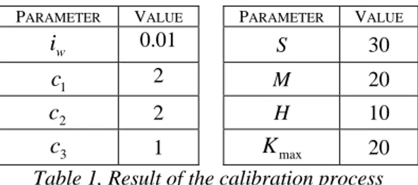
In order to calibrate the set of characteristic parameters of the optimization technique, a linear array of N=20 equally-spaced (d=λ/2) z-oriented dipoles lying on the x-axis has been considered. The amplitudes wn (n=1,…,N) of the array

weights have been chosen according to the Dolph-Chebyshev distribution. Through a large number of simulations, the values reported in Table 1 have been determined.

PARAMETER VALUE PARAMETER VALUE

w i 0.01 _{S 30} 1 c 2 M 20 2 c 2 H 10 3 c 1 Kmax 20

Table 1, Result of the calibration process

In particular, the size M of the buffer has been tuned by considering three different scenarios of interfering sources. The former is a stochastic model, since the arrival time of the jammers is modeled by means of Poisson process with a maximum life-time of 2 iterations [13]. Moreover, the directions of arrivals are randomly distributed in φ∈

[ ]

0,π with

2

π

θ= . At each time-step a random number J of jamming signals impinges the array with a fixed power of above the desired signal, while a background noise with has been considered. The distance of the interferences has been uniformly distributed between 5λ and 100λ.

] [ 30 ) ( dB Pi = P(n)=−30[dB] ) (i j d

The second scenario is the so-called “Scenario 1” used by Weile et al., [5]. Finally, the so-called “deterministic scenario” is characterized by a cluster of interferences whose direction is supposed to be constant for a large number of iterations.

Fig. 1 shows the behavior of the SINR with (M=20) and without memory (M=0) versus the time-steps tl (Lmax =900). As

expected, the most significant enhancement holds for the deterministic configuration, even though the learning capabilities of the approach impacts in a non-negligible way on the other scenarios, as well.

As far as the location of the jamming sources are concerned, the capability to place proper null in the synthesized beam pattern depends on the number of bits B of the digital phase shifters, especially in correspondence with small values of the distance (i). Fig. 2 shows the quality index

j d Φav defined as 100 × = Φ − FF FF Full SINR SINR SINR av (15)

where the subscripts (Full) and (FF) indicate that the SINR has been computed using the array weights optimized through (10) taking into account the relationships (2) and (4), respectively. Moreover, in (15) the SINR has been computed neglecting the MC effects (Ψ=

N

I ). When B>8, the binary-solution-space turns out to be too large for allowing fast convergence and reliable results.

Figure 4, SINRFull versus the time-steps for different techniques

Figure 5, SINRFF versus the time-steps for different techniques

Figure 6, mutual coupling effects on the SINR versus the time-step for a planar array

For comparison purposes, the result of Fig. 2 with B=8 by the PSOM has been compared with those of the Applebaum optimal method [2], the optimal method with discrete phases (DPA), the learned real-time GA [12], and the PSO [6]. Fig. 3 clearly indicates that the proposed approach outperforms the LRTGA and the PSO, approaching the behavior of the DPA whatever the jamming location.

Figure 7, mutual coupling effects on the beam pattern for a planar array

When considering a realization of the Poisson scenario ( , ) under the assumption that is a random variable, the behavior of the SINRFull is reported in Fig. 5. Since LRTGA is about 4 times computationally

heavier than the PSO method, has been set to in order to achieve the same reaction time per slot of time tl. The achieved results demonstrate that the PSO-based approach outperforms other optimization methods of

digital ] [ 30 ) ( dB Pi = P(n)=−30[dB] (i) j d ) ( max LRTGA K K_max(PSO)/4

Figure 8, Beam pattern optimized through PSOM

control. For the same scenario, the behavior of the SINRFF is shown in Fig. 5. In this case, the optimal method achieves

almost the same performance of Fig. 4, while the other control methods cannot optimize the beam pattern and properly locate the beam pattern nulls.

The last test case is aimed at evaluating the capabilities of the PSOM in facing the MC effects. A hexagonal planar array of N=61 dipoles with uniform amplitudes for the weights has been considered [14]. Let us consider the SINR computed through (6) with the array weights optimized neglecting the MC effects (i.e., SINR, is obtained by fixing the non-diagonal elements of the matrix Ψ equal to zero) or not (i.e., SINRMC). Fig. 6 shows the behaviors of the two

signal-to-noise-ratios versus the time-step index tl. Neglecting the MC effects causes a visible degradation of the

performances at the receiver, due to the shift of the locations of the nulls in the beam pattern with respect to the actual directions of arrival the interferences (Fig. 7, when l=766).

For the sake of completeness, Fig. 8 shows the beam pattern in correspondence with a scenario characterized by two jamming signals [

(

, , ()

)

(

87,128,15

)

1 ) ( 1 ) ( 1 = i i i d θ φ and

(

, , ()

)

(

147,62,15

)

2 ) ( 2 ) ( 2 = i i i

d θ φ ]. The interferences are correctly cancelled by

means of a couple of nulls, -59[dB] in depth, placed in proper directions.

4. CONCLUSIONS

This paper illustrates an innovative technique based on an enhanced optimization strategy for the adaptive control of phased array in complex scenarios.

The numerical validation, carried out through different array geometries and in various noisy configurations, confirms that the approach presents: (a) an enhanced computational efficiency allowing an improvement of the convergence rate without increasing the computational burden of the adaptive control; (b) a robustness to both near-field and far-field interferences; (c) the capability to face with and counteract the mutual coupling effects arising in realistic array architecture.

5. REFERENCES

1. M. Chryssomallis, “Smart Antennas,” IEEE Antennas Propagat. Mag., vol. 42, no. 3, pp. 129-136, Jun. 2000. 2. S. P. Applebaum, “Adaptive Arrays,” IEEE Trans. Antennas Propagat., vol. 24, pp. 585-598, Sep. 1976.

3. B. Widrow, P. E. Mantey, L. J. Griffiths, and B. B. Goode, “Adaptive antenna systems,” Proc. IEEE, vol. 55, no. 12, pp. 2143-2159, Dec. 1967.

4. R. L. Haupt, “Phase-only adaptive nulling with a genetic algorithm,” IEEE Trans. on Antennas Propagat., vol. 45, pp. 1009-1015, Jun. 1997.

5. D. S. Weile and E. Michielssen, “The control of adaptive antenna arrays with genetic algorithms using dominance and diploidy,” IEEE Trans. on Antennas Propagat., vol. 49, pp. 1424-1433, Oct. 2001.

6. M. Donelli, R. Azaro, F. De Natale, and A. Massa, “An Innovative Computational Approach Based on a Particle Swarm Strategy for Adaptive Phased-Arrays Control,” IEEE Trans. Antennas Propagat., vol. 54, no. 3, pp. 888-898, Mar. 2006.

7. J. Robinson and Y. Rahmat-Samii, “Particle swarm optimization in electromagnetics,” IEEE Trans. Antennas Propagat., vol. 52, no. 2, pp. 397-407, Feb. 2004.

8. R. Eberhart and J. Kennedy, “A new optimizer using particle swarm theory,” Proc. Sixth Int. Symp. Micro-Machine and Human Science (Nagoya, Japan), pp. 39-43, 1995.

9. I. J. Gupta and A. A. Ksiensky, “Effect of mutual coupling on the performances of adaptive arrays,” IEEE Trans. Antennas Propagat., vol. 31, no. 9, pp. 785-791, Sep. 1983.

10. C. A. Balanis, Antenna Theory. New York: Wiley, 1996.

11. A.J. Fenn, “Evaluation of adaptive phased array antenna far-field nulling performance in the near-field region,” IEEE Trans. Antennas Propagat., vol. 38, no. 2, pp. 173-185, Feb. 1990.

12. S. Caorsi, M. Donelli, A. Lommi, and A. Massa, “A real-time approach to array control based on a learned genetic algorithm,” Microwaves Opt. Technol. Lett., vol. 36, no. 4, pp. 235-238, Feb. 2003.

13. A. Carlson, Communication System. New York: McGraw-Hill, 1987.

14. S. Caorsi, M. Donelli, A. Lommi, and A. Massa, “A real-time approach to array control based on a genetic algorithm”, Microwaves Opt. Technol. Lett., vol. 36, no. 4, pp. 235-238, Feb. 2003.