DIPARTIMENTO DI INGEGNERIA INDUSTRIALE E SCIENZE MATEMATICHE Corso di Dottorato di Ricerca in Ingegneria Industriale – Curriculum Ingegneria Energetica
Ph.D. Thesis
Tools and Methods to study the integration of flexibility assets
in the future Smart Grid
Advisor:
Prof. Gabriele Comodi
Curriculum Supervisor:
Prof. Ferruccio Mandorli
Ph.D. Dissertation of:
This dissertation presents tools and methodologies to support the research commu-nities, as well as industrial entities and policy makers, understanding the role that flexibility assets and aggregators will play in the future Smart Grid.
A Virtual power plant framework for aggregators of flexibility resources is intro-duced, based on two operation levels: the "Local assets level", where the aggregator interacts with the end users collecting data to estimate and control their flexibility, and the "Flexibility Aggregator level", where it interacts with the energy market to buy/sell energy and provide different services. For each level, the aggregators objectives are presented , together with a list of the main open questions/challenges from both the research and industry communities.
A generalized modeling methodology is defined to describe and control the dif-ferent flexibility assets as an equivalent energy storage. Using this formulation it is possible to aggregate the contribution of thousands of heterogeneous assets by eval-uating the single time-variant parameters and summing their relative contribution. A simulation methodology to test the impact of integrating a thermal energy storage with an existing HVAC system is presented, using the School of Art, Design and Media building, located within the NTU campus in Singapore, as case study. Results show how the extra flexibility granted by the energy storage can sensibly im-prove a building performances, reducing reducing operational costs while improving the cooling system efficiency.
The concept of equivalent storage model is introduced and applied to simulate a heterogeneous population of 1000 thermostatically controlled loads. The study demonstrates how moving from a dynamic setpoint strategy towards a dynamic deadband one, consumers could trade energy saving potential to increase their load flexibility. Relaxing the thermostats control deadband, aggregators can replace more storage capacity integrating the same number of residential costumers. Using the same simulation platform, a study on the impact of different climate areas on the aggregated flexibility is presented. Results show how temperate climates get
A novel modeling approach is defined to describe an aggregation of Electric Vehicles System Equipments (EVSEs) as an equivalent energy storage. The model is based on five parameters that can be estimated using historical charging data. These parameters depend on arrival and departure time, the energy consumed driving and the charging frequency. They should be evaluated for each single EVSE and summed up to aggregate their contribution.
Following our studies on flexibility assets modeling, the results from some exper-imental tests performed in an industrial microgrid are presented. A sensible heat thermal energy storage and the existing HVAC system are integrated to reduce the peak load during critical hours. Results show that, when the strategy is revoked and the original temperature setpoint is restored, a new peak is generated in terms of power demand. Also, data show that sampling the electricity consumption with a 15 minutes time granularity is adequate to identify the activation of a load shedding strategy.
The last part of the dissertation focuses on how to optimally manage the aggre-gated capacity gathered from an heterogeneous portfolio of flexibility assets. A methodology is presented to address the optimal portfolio management problem for flexibility aggregators. The methodology integrates the equivalent storage mod-els for flexibility assets in a convex optimization. The goal of the formulation is to optimally manage the available flexibility resources, leveraging the energy price variability to reduce operational costs, while producing valuable services for the national grid. The methodology is tested in two alternative scenarios. Results show that integrating controllable thermostatically controlled loads and electric vehicles in an urban district, we can reduce aggregators need for extra storage capacity by up to 30%, while providing the same level of service. Results highlight how inte-grating EVSEs can have a positive, negative or neutral effect depending on mobility schedules and the required service.
Finally, a multi-agent based control architecture is introduced with the scope of managing the flexibility assets of an industrial microgrid. The control architecture is tested using real data from an Italian industrial facility, simulating the inter-ests of an aggregator which seek to optimally control the different flexibility assets of the microgrid to reduce operational costs and limit consumption peaks during critical hours. Different comparison metrics are introduced to highlight how the effectiveness of the control architecture is affected by the energy price variability.
I do believe that our lives represent the weighted sum of all things that happen to us and, most importantly, of all the people we meet.
Looking back i realize today how lucky i have been. There are moments in life when you need to be in the right place, with the right person, having the right discussion. That very discussion will eventually trigger that something in you, that will change your life forever. I would like to say thanks here to some of these right persons that i have met, persons that without knowing it, contributed in their own way to this thesis.
I would like to thank my academic advisor, Gabriele Comodi, who shared with me his vision of the research world, without ever imposing it. He entrusted me completely, giving me the opportunity to learn my way, exploring my own ideas and intuitions. He pushed me to travel, allowing me to growth as a person and as a researcher.
I would like to thank Cristina Cristalli, Antonio Giovannelli and Gino Romiti which for an extended period of time acted as parents figures, advisors and great sources of inspiration for the passion and the energy they demonstrate every day at work. Thanks to Sila Kiliccote and Emre Can Kara, my technical and spiritual advisors for the period i spent at SLAC, in Silicon Valley. I don’t think they fully realize what they did to me, when they granted me the opportunity to join their research group and work with them. They made me realize one of my life dreams, having the chance to work at Stanford, one of those legendary places that we sometimes hear about in movies and books. Not only that. Through their passion and their advices, they made me realize how much i love doing research and how much i would like to be good at my job. For all of this and much more, i will be eternally grateful to them.
I would like to thank Alessandro Romagnoli, an extremely passionate and skilled researcher, who accepted me in his group in Singapore, giving me the unique op-portunity to confront myself with a completely different culture.
there listening to my rants and worries. The guy is seriously responsible for this thesis, being the one who made me think seriously, for the first time, about going for the Ph.D. position.
Finally, I would like to thank my family. My parents, Stefania and Luigino, my sister, Laura, and my acquired brother Luca. They represent an incredible source of inspiration and love. They always supported me no matter what, regardless of my strange ideas, my being different, and my willingness to explore things in life away, sometimes far away, from home.
Abstract iv
List of Figures xv
List of Tables xvi
1 Introduction 1
1.1 Goals and main contributions . . . 4
1.2 Dissertation Overview . . . 5
2 The Virtual Flexibility Plant for Aggregators 7 2.1 Preface to Chapter 2 . . . 7
2.2 Introduction . . . 7
2.3 Framework description . . . 9
2.3.1 Local assets level . . . 10
2.3.2 Aggregator level . . . 12
2.4 The equivalent storage formulation . . . 13
2.5 Conclusion . . . 15
3 Energy storage systems as flexibility resources 16 3.1 Preface to Chapter 3 . . . 16
3.2 Introduction . . . 16
3.3 Materials and Methods . . . 18
3.3.1 Energy audit . . . 18
3.3.2 Energy storage Modeling and design methodology . . . 24
3.4 Results and considerations . . . 29
3.4.1 Integrating a storage to avoid partial load operations . . . 29
3.4.2 Integrating a storage to replace the backup chillers . . . 30
4 Thermostatically controlled loads as flexibility resources 36
4.1 Preface to Chapter 4 . . . 36
4.2 Introduction . . . 36
4.3 Methodology . . . 39
4.3.1 Individual TCL model and flexibility . . . 39
4.3.2 TCLs characteristics . . . 41
4.3.3 Simulation setup . . . 42
4.3.4 Thermostat control strategies . . . 43
4.4 Results . . . 44
4.5 Conclusions and next steps . . . 46
5 Electric vehicles as flexibility resources 49 5.1 Preface to chapter 5 . . . 49
5.2 Introduction . . . 50
5.3 Controlled vs uncontrolled charge . . . 52
5.4 EV equivalent energy storage model . . . 54
5.4.1 Using the equivalent energy storage model . . . 56
5.5 The impact of mobility patterns on the aggregate flexibility . . . 57
5.6 Conclusions . . . 58
6 Flexibility resources in an industrial microgrid 60 6.1 Preface to chapter 6 . . . 60
6.2 Introduction . . . 60
6.3 Methodology . . . 61
6.3.1 The industrial microgrid . . . 62
6.3.2 The HVAC system . . . 62
6.3.3 The thermal storage . . . 63
6.3.4 Demand side management strategies . . . 63
6.4 Results . . . 63
6.5 Conclusions . . . 67
7 An Optimal Portfolio Management Framework for Flexibility As-sets Aggregators 68 7.1 Preface to chapter 7 . . . 68
7.3.2 Flexibility estimation . . . 73
7.3.3 Convex formulation for flexibility assets optimal dispatch prob-lem . . . 76
7.3.4 Dataset description . . . 81
7.4 Results . . . 84
7.4.1 The aggregator bidding problem . . . 84
7.4.2 The district’s ramp rate control problem . . . 85
7.5 Conclusions . . . 91
8 A multi-agent based control architecture for flexibility assets in industrial microgrids 93 8.1 Preface to chapter 8 . . . 93
8.2 Introduction . . . 94
8.3 Methodology . . . 97
8.3.1 The Multi-agent based control architecture . . . 97
8.3.2 Test case: the industrial microgrid . . . 102
8.3.3 Simulation setup . . . 103
8.3.4 Comparison metrics . . . 106
8.4 Results and discussion . . . 108
8.4.1 Possible improvements and future steps . . . 110
8.5 Conclusions . . . 111
9 Conlusions 113 9.1 Key findings and impact . . . 113
9.2 Future research topics . . . 116
2.1 The Virtual Flexibility Plant architecture for aggregators . . . 10
2.2 The equivalent energy storage model. . . 14
3.1 Model of the building’s cooling system . . . 19
3.2 Cooling load profiles in March 2015 . . . 21
3.3 Cooling load profiles in April 2015 . . . 22
3.4 Cooling load profiles in May 2015 . . . 22
3.5 Cooling load profiles in June 2015 . . . 22
3.6 Coefficient of Performance of the cooling system . . . 23
3.7 Cooling load profile for a normal operative day . . . 23
3.8 Energy storage model . . . 25
3.9 Typical CTES system’s configuration . . . 26
3.10 The new cooling system integrating the CTES . . . 29
3.11 New cooling load obtained ntegrating a storage to avoid partial load operations . . . 30
3.12 New cooling load obtained using a storage to replace the backup chillers 31 3.13 New cooling load obtained Integrating a storage to arbitrage the en-ergy price . . . 33
4.1 The boxplots represent the parameters distribution for the simulated population of households. . . 42
4.2 Median temperature profiles for Sacramento, Los Angeles and Las Vegas . . . 43
4.3 Power and indoor air temperature profiles generated using different thermostat control strategies. . . 44
4.4 The effect of different control strategies over 1000 simulated house-holds in terms of cooling load. . . 46
5.1 Net-load profile from Pecan Street Dataset . . . 53
5.2 Net-load profile from Pecan Street Dataset considering PV generation 53 5.3 Net-load profile from Pecan Street Dataset considering PV generation and EV charge . . . 53
5.4 Storage parameter evolution for two EVSEs over 24 h period. . . 57
5.5 Mobility patterns and storage parameters . . . 58
6.1 Building net-load with 15 minutes granularity . . . 64
6.2 Effect of the thermal energy storage on the electricity demand . . . . 64
6.3 Heat pumps’ consumption profile during five working days . . . 65
6.4 Heat pumps’ consumption profile windowed around the testing time 66 7.1 The Flexible Assets Portfolio Management Framework in its three main components. . . 73
7.2 The equivalent energy storage model. . . 74
7.3 The simulated district original Net-load . . . 82
7.4 Price vector from the ERCOT Real-time energy market . . . 83
7.5 (a) and (b) shows the original and final net-load, together with the tracking profile. (c) and (d) the relative optimal flexibility assets dispatch profile. . . 86
7.6 Internal energy trend for the EES (a), TCL equivalent energy storage (b) and EV equivalent energy storage (c) . . . 87
7.7 Sensitivity Analysis over EES cost . . . 88
7.8 (a) shows the original and final net-load. (b) shows the relative op-timal flexibility assets dispatch profile. . . 89
7.9 The two histograms highlight the effect of the flexible loads in limiting the ramp rates . . . 89
7.10 Sensitivity analysis plots showing how the optimal storage size varies with controllable TCLs (a) and EVs (b) penetration level . . . 91
8.1 Multi-agent based control architecture. . . 99
8.2 Loccioni’s microgrid consumption (a) and generation profiles (b,c), May 2016. . . 103
non-critical (in yellow) share of loads. . . 105 8.4 Energy price input vectors representing the PUN (a) and the BM (b)
in May 2016. . . 107 8.5 Focus on the control mechanisms response to a dynamic price vector 108 8.6 Baseline power, shifted power and energy price profiles for scenario
3.1 Chillers specs . . . 20
3.2 Chilled water pumps specs . . . 20
3.3 Cooling towers specs . . . 20
3.4 Cooling towers specs . . . 20
3.5 Cooling energy demand of the building . . . 26
3.6 Main results obtained using a storage to avoid partial load operations 30 3.7 Main results obtained ntegrating a storage to replace the backup chillers 32 3.8 Main results obtained integrating a storage to arbitrage the energy price . . . 33
6.1 Data from November tests . . . 66
8.1 Batteries specifications. . . 104
8.2 Scenarios definition. . . 106
Introduction
The way we generate, control and distribute energy has always been one of the pivotal problems for the human race. Men in caves used fire to generate heat and satisfy their primary demands: heating their caves and cooking their food. Along the centuries we evolved, together with our lifestyle and the nature of our neces-sities: we need light to work and study at night; cooling energy to maintain food for longer periods; mechanical power to move complex machineries. The industrial revolutions first, and the discovery of electricity later, represented a paradigm shift that change the way we thought about energy generation and consumption. These pivotal moments set the cornerstones of the XX century society. All over the world, countries started investing in fossil fuel power plants, in transmission and distribu-tion networks to sustain the growth of energy demand coming from industries and the new cities.
The XX century power grids requirements are quite simple: deliver cheap, reli-able electrical power to everyone. XX century power grids are mostly based on big thermal power plants, powered by fossil fuels, and unidirectional transmis-sion/distribution networks, designed to reliably transmit power from generation sites towards final users [87]. This paradigm, that worked fine for over a century, is now challenged by a new set of requirements. The future power grids need to deliver clean, cheap and reliable electrical power to everyone [56]. To make human presence in this planet sustainable, we need our power generation and distribution systems to be sustainable. This means shifting from fossil fuels towards alternative, clean source of energy.
In the last two decades we have seen renewable generation technologies, such as PV solar and wind turbines, getting introduced into every nation’s energy mix, in both centralized, large power plants in the order of decades of mega-Watts, and
distributed way, rooftops solar in the order of decades of kilo-Watts. This trend is now stronger than ever, thanks to the ambitious goals that many countries of the world are posing to reduce GHG emissions and record low auction prices, which are making renewable generation every day more competitive. A recent report from the International Energy Agency shows how solar PV installed capacity grew by 50%, about 74 GW, in 2016 alone [55].
The 2016 Paris agreement goes towards this direction, committing industrialized nations to reduce GHG emissions 80% below 1990 levels by 2050. A recent study from E3 indicates a possible pathway to achieve these goals, highlighting how we need to decarbonize the energy generation mix and push for the electrification of our services, from the residential to the mobility sector [86]. Our services’ demand is already becoming more and more dependent from the electrical grid, due to novel technologies which are gradually being introduced. Highly efficient Heat pumps use electricity to generate both cooling and heating energy, substituting natural gas that was used for heating purposes. Plug-in electric vehicles aim to contribute to the electrification of both private and commercial mobility sector, reducing our dependency from fossil fuels while affecting the air quality in our cities. These transformations, which are widely recognized as positive first steps towards our path to decarbonization and a more sustainable future, also represent serious challenges for the energy distribution network. They are forcing us to rethink the way we design and operate power grids, which as today are not ready to cope with many of these new technologies.
Power grids are designed to work under balanced supply and demand at all times. This hard constraint is increasingly challenged by uncertain and intermittent renew-able generation sources. Historically, grid balance was maintained by operating the controllable thermal generators, dispatching the so called peaker plants which can be ramped up and down at will. These power plants, which remain idle for the majority of the time, are used to balance the demand, sustain power reliability, compensate for grid’s frequency and voltage oscillations. This is what we call a "demand following" paradigm: we operate the available peaker plants to cope with the energy demand variance at all time. If the peak demand grows, we build new peaker plants to cope with it.
This paradigm is being challenged by the growth of the peak demand to respect with the average demand. The combined effect of residential loads electrification and the adoption of distributed PV generation, generate a stiff ramp in the national net-load demand during late afternoons, when people goes home from work and
PV production start decreasing. We can see this happening around the world. In California this issue is referred as the Duck Curve problem: CAISO (Californian In-dependent System Operator) estimated that California’s late afternoon ramp needs will increase up to 13 GW by 2020 [18]. Therefore, the system requires a flexible resource mix that can react quickly and balance the fast changes in electricity net demand, avoiding reliability issues. However, an MIT study, based on 2005-2009 data, demonstrates how peaker plants are not anymore a sustainable solution. The study shows how in the states of New England and Washington, the national de-mand of energy exceeded 70% of its peak for only about 1000 hours per year, so that more then 30% of the installed capacity was in use less then 12% of the time [73]. Leaving aside the environmental standpoint, this trend makes peaker plants less and less appealing also from the economic perspective.
The Smart Grid paradigm offers an alternative solution to this problem by shift-ing part of the control burden from the generation to the demand side. The Smart Grid combines advancement in information technology, power systems, energy sys-tems engineering and data analysis to increase the power grid reliability. It works by leveraging data to better manage grids’ resources, remotely controlling a port-folio of distributed technologies so that they can actively respond to changing grid conditions [58].
The Smart Grid implies a Copernican revolution from the perspective of the old paradigm: we operate on the energy demand to cope with the variability of our energy mix. Technically, we move part of the control burden from the centralized generation systems to end users, incentivizing a diverse use of energy to reduce the need for extra peaker plants. In this new paradigm, consumers play a more active role, which is now possible thanks to the diffusion of low cost advanced metering infrastructure and distributed technologies, such as remotely controllable inverter, rooftop PV solar and electric energy storage systems.
Demand response programs were designed to engage end users and promote this new paradigm. They aim to increase the distribution network flexibility using a bot-tom up approach, aggregating distributed energy resources (DER) to maintain the grid balance during critical hours. In exchange for using their resources, end users get rewarded with economic benefits or services [82]. In this dissertation, we use the term "Flexibility assets" to indicate DERs which can be coordinated and controlled to reshape the energy demand at distribution level, providing extra flexibility and services to the national grid (e.g. electric energy storage systems (EES), distributed generation plants, as well as interruptible residential and industrial loads).
These flexibility assets are characterized by their relative small capacities with re-spect to the centralized generation, and they are connected to low and medium voltage electricity distribution grids. Thus, while they have huge untapped poten-tial, they need to be aggregated to functionally replace peaker plants in delivering valuable electricity services. The Aggregation process is defined as the effort of grouping distinct agents in a power system (i.e. consumers, producers, storage as-sets) to act as a single entity when interacting with an energy market [15]. This effort is coordinate by a new player in the energy market, the aggregator. Aggre-gators are companies who act intermediary between end users and DER owners that are willing to offer their capacity in exchange for benefits, and the power grid participants which are willing to pay for the extra capacity [51].
Throughout this dissertation we will talk about flexibility assets, developing models, methodologies and tools that can help us imagine their role in the future energy distribution system. We will look at the problems from the prospective of an aggregator, addressing some of the open questions that must be answered before the Smart Grid vision becomes a reality.
1.1
Goals and main contributions
The main goal of this dissertation is to introduce tools and methods to support the research community, as well as industrial entities and policy makers, understanding the role that flexibility assets and aggregators will play in the future Smart Grid.
This research field, while being in constant expansion and evolution, is already extremely wide and complex. For this reason we decided to narrow the scope of this work, defining our own vision for flexibility aggregators and focusing on three specific types of flexibility assets: energy storage systems, thermostatically controlled loads (TCLs) and electric vehicles (EVs).
The aggregator we envisioned is interested in the direct load control approach to demand response, as opposed to the indirect one. The Direct load control paradigm sees the aggregator as a central entity developing and enforcing automated con-trol strategies to dispatch the distributed assets which are part of its portfolio of resources; on the other hand, the indirect control approach wants to trigger behav-ioral changes in the end users by setting an exogenous stimulus, e.g. a new energy price tariff that penalizes specific hours of the day. We believe the former approach to be more interesting due to its characteristics, which make it suitable for a wide
range of grid services and demand side management applications, from slow ones (e.g. price arbitrage in the day ahead market) to really fast one (e.g. grid primary regulation) [59].
Our main contributions to the state of the art are the following:
• We introduce a Virtual Power Plant architecture for Aggregators interested in performing direct load control of flexibility assets.
• By simulating an heterogeneous population of 1000 TCLs, we demonstrate how a control strategy based on deadbands relaxation can significantly in-crease the aggregated demand flexibility at the expense of energy efficiency. • We define a modeling approach to describe and control an aggregate of EVs
charging stations as an equivalent energy storage.
• By performing tests in an industrial microgrid, we demonstrate that it is possible to identify the activation of a peak reduction strategy using electricity consumption data collected with a 15 minutes time granularity
• We define a methodology to solve the optimal portfolio management problem for flexibility aggregators, using the equivalent energy storage models devel-oped for the different flexibility assets within a convex formulation
• We present a multi-agent based control mechanism tailored over the necessities of an industrial microgrid.
1.2
Dissertation Overview
In chapter 2, we introduce the Virtual Flexibility Plant framework for aggregators. We distinguish between two operation layers for the aggregator. Each layer brings its own open questions to be answered and challenges to be handled. Also, in this chapter we present four different categories of flexibility assets, highlighting the importance of introducing a general modeling formulation.
In chapter 3, we present a study on the effect of a thermal energy storage when coupled with an existing Heating Ventilating and Cooling (HVAC) system. In par-ticular we show how we can use the extra system flexibility to better manage the heat pumps and increase the overall system efficiency.
In chapter 4, we implement a methodology to estimate the technical potential of an aggregation of heterogeneous TCLs in providing demand response (DR) services.
We use this methodology to assess the effect of different control strategies, and different climate conditions, on the flexibility estimation.
In chapter 5, we focus on EV. We first discuss about risks and opportunities related to a potential shift from fossil fuel based mobility towards EV. Then we introduce an equivalent storage model for aggregations of EV charging stations.
In Chapter 6, we present some preliminary results obtained by introducing some advanced demand management strategies in an industrial building. These strategies aim to control the HVAC system and the local thermal energy storage to reduce the building load during peak hours of the day.
In chapter 7, we introduce an optimal portoflio management strategy for flexibility aggregators. We use it to optimally size the flexibility assets in the portfolio or, given a fixed portfolio, to obtain the optimal dispatch profile. The framework uses an equivalent energy storage approach to model the different assets of a potential portfolio (Energy storages, EVs, TCLs). We present a general convex formulation to address the optimal dispatch problem.
In chapter 8, we introduce a multi-agent based control architecture to efficiently dispatch the flexibility assets of an industrial microgrid, based on DER availability and time-of-use rates (TOU). We use actual consumption and generation data from an Italian industrial microgrid and energy prices from different markets. The study aims at highlighting the potential of such a control architecture and the impact of the energy price.
In chapter 9, we conclude discussing the results we obtained and the impact we expect for our research. We also suggest some future research path that can poten-tially develop from our work.
The Virtual Flexibility Plant for
Aggregators
2.1
Preface to Chapter 2
In this chapter we introduce the Virtual Flexibility Plant framework for aggregators of flexibility assets. We first present the related literature on the topic, then we introduce the framework to describe the different tasks that the aggregator faces at both the end users and aggregate levels. We use the last portion of the chapter to introduce the general idea of equivalent storage formulation, explaining its crucial role when modeling the different flexibility assets. Many of the concepts introduced here will be referenced later throughout the thesis.
2.2
Introduction
The electrical distribution system is facing significant changes from both the gen-eration and the demand prospectives. From the gengen-eration side we introduced new distributed generation capabilities, intermittent renewable sources and new, more and more affordable, ways to store energy. From the demand side we are seeing a new electric loads coming from the residential, industrial and even the mobility sector. Distributed energy sources (DERs) are connected to the low and medium voltage distribution grids and are characterized by smaller capacity with respect to the centralized units. Their primary goal is to provide reliable, stable, power to local users, however their distributed nature enables a new set of services towards both the final user and, once aggregated and coordinately controlled, the entire distribution grid. Many studies from recent literature focus on the technical
po-tential of DERs, energy storage systems and demand response strategies that, once aggregated, can generate benefits for the distribution grid and value streams for the end user. In [71] authors describe a method to estimate the technical potential that California could leverage aggregating residential TCLs to provide frequency regulation and spinning/nonspinning reserve. In [61] authors estimate the poten-tial benefits of aggregating large numbers of electric vehicles charging stations to optimally coordinate their charging strategy based on a time of use (TOU) rate structure. To untap the full potential of these controllable distributed resources, to make them observable and controllable, we must integrate them with smart sensors and information technologies. Aggregators play a critical role as enablers, being both the technology providers and the ones interested in using the untapped po-tential to contract services with the grid. Aggregators are service and technology providers, facilitating an active participation of end users and DER owners with the energy market. They form a portfolio of consumers, distributed generation sys-tems and controllable assets (e.g. DERs, energy storage) that must be optimally managed with respect to an energy market. In [15] authors explore the value of aggregation, distinguishing among different categories of them, showing how differ-ent regulatory and market frameworks can be leveraged by aggregators to generate value for them-self, for end-users and the entire distribution system. For example, they can assume the basic role of retailers for their end users, while creating a value stream for all the flexible assets and prosumers who wants to act as distributed grid resources [14]. From the national grid prospective, the aggregator portfolio of consumers, generators and storage represents a virtual power plant: an additional backup resource that can be dispatched for a price. Virtual power plant (VPP) aggregate distributed generation units, consumers and energy storage systems cre-ating an ICT infrastructure to allow the continuous exchange of data. VPP main goal is to optimally manage the distributed resources by trading the overall capac-ity in an energy exchange platform. In recent years this vision of Virtual Power Plants made by the aggregated contribution of many distributed assets have been garnering interest in the research community. We suggest the interested reader to refer to the work of Nosratabadi et al. [79]. They present a comprehensive review of the concept of virtual power plant in relation to the one of microgrid and dis-tributed resources. They also study the optimal scheduling problem, analyzing the state of the art in all its aspects: modeling techniques, solving methods, objectives. In this chapter we introduce a VPP framework for flexibility aggregators. We refer to it as the Virtual Flexibility Plant (VFP). The VFP represents the aggregation
mechanism we envisioned. We distinguish between two operational layers for the aggregator, Each one with its own open questions to be answered and challenges to be handled. Also, in this chapter we present four different categories of flexibility assets, highlighting the importance of introducing a general modeling formulation.
2.3
Framework description
Figure 2.1 shows our framework for aggregators of flexibility assets, we call it Vir-tual Flexibility Plant (VFP). We need to introduce four entities to describe it. The aggregator has a central lore. It represents the company, or institution, which works as facilitator between the distributed flexibility assets, that can provide distributed flexibility increasing/reducing the consumption capacity, and the energy market which requires such extra capacity. We refer here to energy market as a generic entity which is representative of one or more market frameworks. The aggregator can interact with all of them to buy energy, bid its virtual capacity and price its ser-vices. The Minimum flexibility units represent grid nodes over which the aggregator has observability and, in specific cases, direct control. These nodes represent point of connection between the end users and the main grid. Each Minimum flexibility unit is associated to one smart meter. The aggregator has no observability over anything that happens behind this meter. The flexibility assets represent the differ-ent kinds of resources that can provide extra flexibility to the end user demand and, through the aggregator, to the distribution network. Throughout this dissertation we are going to focus on three kinds of flexibility assets: energy storage systems, controllable TCLs and electric vehicles. The VFP is a combination of distributed generation units, controllable load and energy storage systems that are aggregated to trade their flexibility for money and reduce their cost of operation. The ag-gregator, which control the VFP, can coordinate its assets to arbitrage the energy price, by buying more energy during low price hours and bidding its extra capacity during peak hours. Alternatively, it can use its resources to sell specific services to the grid. For example, the fast reactive assets of the portfolio (such as TCLs and energy storage) can be dispatched to provide frequency regulation services. The aggregator we envision operates at two distinguished levels: the "Local assets level", where it interacts with the end users collecting data to estimate and control their flexibility, and the "Flexibility Aggregator level", where it interacts with the energy market to buy/sell energy and provide different services.
Figure 2.1: The Virtual Flexibility Plant architecture for aggregators
2.3.1 Local assets level
At the "local assets level", the aggregator establish a peer-to-peer communication channel with each Minimum flexibility unit. From the aggregator prospective each Minimum flexibility unit corresponds to an asset of its portfolio of resources. The aggregator needs observability and controllability over these nodes of its network, thus each of them requires an appropriate advanced metering and communication infrastructure. At any given time, the aggregator needs data on nodes’ net-load, which represents the amount of power exchanged with the grid through the metering points. Throughout this work we consider positive net-load when the power is flowing from the main grid towards the end user, which means that behind the meter the demand is greater then the local generation; we consider negative net-load when the power is flowing from the end user towards the main grid, which means that local generation is exceeding the demand. The "Minimum flexibility unit" is an abstraction that represents different types of resources as nodes of the aggregator’s portfolio. The Minimum flexibility unit is always associated to a single meter but, depending on the aggregation level, it can be representative of a single flexibility asset (e.g. an energy storage system, a cogeneration plant), a single end user (e.g. an household), multiple end users (e.g. an urban district) or an industrial microgrid. With the "minimum flexibility unit" abstraction, the aggregator is not interested in how complex is the energy network behind a specific meter. Using
historical data, the aggregator evaluates the natural behavior, the baseline, of each node. The baseline is then used as a reference to estimate nodes’ flexibility in terms of how much they can variate their power consumption with respect to their natural behavior.
At the Local assets level the aggregator is interested in the following actions: 1. Enable the different Minimum flexibility units by providing the necessary
ad-vanced metering infrastructure to ensure observability and control 2. Estimate the baseline behaviour of each Minimum flexibility unit 3. Estimate the flexibility that each Minimum flexibility unit can provide Both the academic and industrial research communities are working on solving a se-ries of challenges in relation to these services. To begin with, aggregators need data from the Minimum Flexibility Units. It is critical to define standards and protocols to install the appropriate advanced metering infrastructure at the local level. This problem involves different fields. The required set of sensors and communication devices should be advanced enough to ensure observability and control, while being affordable to allow aggregators to build a business model out of their services [57]. Moreover, it is crucial to define safety protocols and communication standards to ensure end users privacy and cyber-security [64].
Once data is obtained, aggregators can move further and estimate, for each min-imum flexibility unit, the baseline behavior and the potential flexibility that can be provided. This process involves a modeling effort to transform, for each node, historical and real time data into flexibility insights. All these modeling tasks are necessary to build simulations, define and tests management strategies at both the local assets’ and aggregator’s levels. These simulations can also be used for tar-geting purposes, analyzing alternative sets of locations and end users to find the optimal location for the aggregator to invest and propose its services. In this dis-sertation we choose to focus on the modeling and simulation tasks, defining specific methodologies to study the impact of different flexibility assets at both local and aggregate level. To limit the scope of the research we choose to focus on three kinds of flexibility assets. Chapter 3 is dedicated to energy storage systems, chap-ter 4 to thermostatically controlled loads and chapchap-ter 5 to electric vehicles. We briefly introduce the topic of the metering infrastructure in chapter 6, when we talk about data granularity in demand side management applications, referring to some experimental tests we performed in an industrial microgrid.
2.3.2 Aggregator level
At the "Flexibility Aggregator level", the aggregator exchanges data with all the "Minimum flexibility units" of its portfolio to estimate the available flexibility, send control signals and observe the assets response. At the same time, it interacts with the energy market to buy/sell energy and value its aggregated flexibility. The aggregator final goal is to generate value for itself and to the end users which are part of its portfolio by optimally managing their flexibility resources. Aggregating multiple controllable assets, the aggregator accumulates flexibility which can be leveraged to change its market position and provide different kind of services to the national grid. For example, in the case of a residential district, by asking the final users to reduce their net-loads the aggregator dispatches virtual positive capacity; from the national grid prospective the overall energy demand decreases momentarily. By asking to the final users to reduce their net-load the aggregator dispatches virtual negative capacity; from the national grid prospective the overall energy demand increases momentarily. At the Local assets level the aggregator is interested in the following actions:
1. Estimate the aggregated flexibility that its portfolio of assets can provide 2. Identifie the optimal portfolio management strategy using energy price and
resource availability forecast to make inform decisions
3. Once identified the optimal strategy, send control signals to the single Mini-mum flexibility units to dispatch them
4. Verify that each Minimum flexibility unit is actually able to follow the control strategy using real time data and the baseline model
Also at this operational level, there are many challenges that need to be addressed to enable the vision we have for large scale aggregators. Research need to de-fine the necessary data infrastructure, which mean a generalizable data model, data exchange protocols and a functional, scalable and secure database architecture. Ag-gregators are also interested in how to build and optimally manage their resource portfolios depending on the aggregation scale, market conditions, technical con-straints and required services. Another interesting series of problems are related to the development of business strategies to generate value for the end users, while providing a service for the national grid and ensuring a profit for the aggregator. Here, researcher in the field of multi-agent programming and game theory are work-ing to simulate how different remunerative strategies could work to incentivize the
aggregation of end users in coalition, so that they could be willing to offer their flexibility in exchange for money or extra services. For example, Chalkiadakis et al. adopted a similar approach to design a pricing mechanism to incentive fair and efficient cooperative Virtual Power Plants [22].
In this dissertation we focus on how to optimally manage a portfolio of flexibility assets. In particular we introduce and apply two alternative approaches, tailoring them over the requirements of different aggregation levels. In chapter 7, we define a convex formulation to solve the optimal portfolio management problem, applying it to an urban district. In chapter 8, we present a multi-agent based control mechanism to manage the assets of an industrial microgrid.
2.4
The equivalent storage formulation
As we discussed in the previous paragraphs, Aggregators want to observe the status, aggregate and control the different flexibility assets of its portfolio. The nature of aggregator’s portfolios could be extremely heterogeneous, integrating together different kinds of flexibility assets: office loads through smart plugs, air conditioners through thermostats, EVs through the relative charging stations. Furthermore, depending on the aggregation level the portofolio could refer to the aggregated resources of a local microgrid with a single point of connection with the national grid, an urban district or a regional area with lots of points of connection. For each asset of the portfolio, the aggregator needs to evaluate the relative flexibility, in terms of how much the energy demand of the asset can increase/decrease in respect with the baseline, and the associated cost for the resource dispatch. The Virtual Flexibility Plant Framework introduces an higher abstraction layer in order to model different flexibility assets, and refer to different aggregation levels, using the same formulation. An energy storage system is a machine which stores energy in different forms to increase the level of control over a system. From the grid prospective, it can be considered as a flexibility generator. We can completely define its behavior by knowing its state of charge (the internal energy content to respect with its maximum capacity), its dissipation rate and the amount of power which is being charged/discharged (figure 2.2).
Figure 2.2: The equivalent energy storage model.
It seems natural to imagine every other flexibility asset as a particular case of an energy storage system, described by the same parameters while constrained to follow different sets of physical rules. Our Virtual Flexibility Framework uses a general equivalent energy storage formulation to model the contributions of all the different flexibility assets. In doing so we extend the generalized battery concept presented in [49]. Our equivalent storage model is defined by a set of signals U(t) that satisfy the following equations:
− η− <= U(t) <= η+ x˙t= −αxt− U(t) |x(t)| <= C (2.1)
Where η+ and η− represent respectively the maximum charging and discharging
rates of the equivalent energy storage system; the state variable x represents the in-ternal energy of the system; α is the dissipation rate, the amount of energy naturally lost due to storage inefficiencies, and C the total energy capacity of the equivalent system. We can use this formulation to model and control a generic flexibility re-source as a storage. To describe a generic flexibility rere-source using its equivalent storage form, we need to define how to extrapolate the four equivalent storage pa-rameters (energy capacity, maximum charging/discharging power, dissipation rate) using real time and historical data. This task can be more or less straightforward depending on the flexibility resource nature. As an example, in the case of residen-tial air conditioners the equivalent storage capacity is related to the thermal mass within the thermostat deadband; the state of charge can be associated to the rela-tive distance between the indoor temperature and the comfort limits; the maximum charging rate is equivalent to the maximum cooling capacity of the machine; the dissipation rate is related to internal and external heat gains. Using this formu-lation, we can aggregate the contribution of thousands of heterogeneous assets by simply summing the equivalent storage parameters. Thus, we are able to describe and control radically different kinds of portfolio using the same set of modeling
and optimization tools. Later in this dissertation we are going to present how to estimate the equivalent storage parameters for an aggregation of controllable TCLs and EVs, respectively chapters 4 and 5.
2.5
Conclusion
In this chapter, we introduced the virtual flexibility plant framework for aggregators. The framework is based on two operation levels: the "Local assets level", where the aggregator interacts with the end users collecting data to estimate and control their flexibility, and the "Flexibility Aggregator level", where it interacts with the energy market to buy/sell energy and provide different services. For each level we presented the aggregators objectives, its activities and a list of open questions/challenges from both the research and industry worlds. We explained the reasons behind the need for a generalized modeling methodology and presented the equivalent storage formulation for flexibility assets. Using this formulation, we can aggregate the contribution of thousands of heterogeneous assets by simply summing the equivalent storage parameters. Thus, we are able to describe and control radically different kinds of portfolio using the same set of modeling and optimization tools. In the next chapters we will talk about different flexibility assets, showing how they can be integrated at different levels of the distribution grid and provide different kinds of services.
Energy storage systems as
flexibility resources
3.1
Preface to Chapter 3
In the last chapter we talked about the Virtual Flexibility Plant framework for ag-gregators. We used the framework to introduce the main research questions that we will face throughout this dissertation. With this chapter we begin discussing about the different flexibility assets. Specifically, we focus on energy storage sys-tems, showing how they can be integrated with existing HVAC plants to increase the flexibility of the system and produce economic benefits. This chapter has been published as follows: "G.Comodi, F.Carducci, N.Balamurugan, A.Romagnoli; Ap-plication of Cold Thermal Energy Storage (CTES) for building demand management in hot climates. Applied Thermal Engineering (2016), V. 103 pp. 1186-1195". I undertook the majority of work related to this chapter, including all the modeling tasks, the development of a simulation platform and the interpretation of results. Mr. Balamurugan provided some preliminary analysis on the dataset. Assistant professors Comodi and Romagnoli contributed with comments on the ideas pre-sented and editorial assistance.
3.2
Introduction
Climate change is unequivocal. Each of the last three decades has been successively warmer than any preceding decade since 1850, and the concentration of Greenhouse Gases have increased. Society can reduce the carbon intensity of energy services, pushing the transition toward low-carbon and/or carbon-neutral technologies [39].
Buildings will play an important role since they represent around 40 percent of world energy demand and 25 percent of global water demand, while producing one third of total GHG emissions [36]. Energy demand for building cooling will be one the main causes of the growing energy consumption of developing countries located in hot/tropical climates, hence major efforts are necessary to limit their energy de-mand. Demand Side Management is a mean to increase the efficiency of an entire power system, from generation to the end use, optimizing resources allocation, lim-iting the peak demand, shaping the loads depending on the necessity of the grid [94]. In this context, Thermal Energy Storage (TES) is becoming more and more inter-esting, since it currently represents one of the most cost-effective solutions to enable demand management strategies [4]; TES enables storing thermal energy (either heat or cold) through a storage medium capable to release the required amount of energy when needed [34]. Several studies demonstrated the effectiveness of such systems in different contexts. Cabeza et al. [16] showed the CO2 mitigation potential of TES systems for different applications (refrigeration, solar power plants, passive system in buildings, greenhouses, dishwashers) and countries. They emphasize the importance of analysing each scenario separately, since different applications impact the energy system in different ways and the results can be heavily affected by the energy mix of the reference country. Arteconi et al. [5] described an existing instal-lation of TES in Italy and performed simuinstal-lations to prove the potential of different Demand Side Management strategies. Their results showed that the use of TES leads to an increase in energy demand, while costs decrease proportionally with the difference between peak and off-peak energy rates. Schreiber et al. [90] reported the performance of absorption thermal energy storage combined with cogeneration for industrial applications: they proved that, when appropriately integrated with low grade heat sources, TES has the potential to increase the energy efficiency of the industrial process, reducing the primary energy consumption up to 25%. Chvala [25] presented a technical assessment of TES technology to investigate the potential in U.S. federal buildings sector, concluding that TES is a feasible solution for this category of buildings: thus, TES should be taken into consideration when retrofitting and/or replacement of chillers is carried out. Ora et al. [80] proved the benefits, both energetic and economical, of using a combination of TES and direct air free cooling to satisfy the energy demand of a 1250 kW data centre. The use of direct free cooling is shown to be feasible by itself, however, when using TES in combination with an off-peak electricity tariff, the operational cooling cost can be further reduced. Deforest et al. [32] investigated the economic benefits of sensible
heat thermal energy storage by simulating its application, for an office building, in four different locations spread across the world (Miami, Lisbon, Shanghai and Mumbai). Their results showed the potential of TES systems in reducing the an-nual electricity costs (5-15%) and peak electricity consumption (13-33%). All these studies concur to establish that the feasibility of TES applications is related to eco-nomic and climatic conditions such as electricity rates/regulations and duration of cold/hot seasons respectively. In this chapter we focus only on cold thermal energy storage (CTES) applied in hot climate. In particular, we propose a techno-economic methodology to size CTES according to different management strategies: peak load management, price arbitrage and replacement of chillers’ partial load operations. The last strategy is particularly interesting since it demonstrates how, under certain conditions, CTES can be used to increase the overall efficiency of the cooling system. We investigate the viability of CTES for building demand management purposes in hot climates. We propose a case study using data from the School of Art, Design and Media (SADM), located within the Nanyang Technological University (NTU) campus in Singapore. We develop and apply a deterministic model to evaluate the impact of integrating the CTES with the existing cooling system. In the first part of the chapter, we outline the case study, describing the building, cooling plant, energy demand and enhancement opportunities in terms of cooling system efficiency. In the second part, we describe the sizing methodology, the modeling technique, and the different scenarios of interest. Finally, we discuss the results of the techno-economic analysis.
3.3
Materials and Methods
3.3.1 Energy audit
The climate in Singapore
Singapore lies just north of the Equator near Latitude 1.5 deg N and Longitude 104 deg E. Due to its geographical location and maritime exposure, Singapore climate is characterized by uniform temperature and pressure, high humidity and abundant rainfall. There is not a distinct wet or dry season: maximum rainfall occurs in December and April, while the drier months are usually February and July. Daily temperature usually ranges between a minimum of 23-26C and a maximum of 31-34C with extremes of minimum of 19.4C and maximum of 36C. With regards to ambient relative humidity (R.H.), the daily R.H. spans between 90% (and above) in
Figure 3.1: Model of the building’s cooling system
the early morning and 60% in the mid-afternoon; the mean value is 84% but during prolonged heavy rain, relative humidity often reaches 100%.
Cooling system description
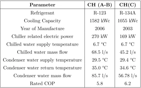
The School of Art, Design and Media (SADM) was built in 2007 as an institutional building with offices, laboratories, libraries, studios and lecture theaters. The build-ing is located inside the Nanyang Technological University campus. Air condition-ing for the buildcondition-ing is provided by three water chillers, as represented in figure 3.1. Chillers (CH) A and B are fitted with centrifugal compressors, using R-123 refrig-erant, having a cooling capacity of 1582 kW each. Chiller C is fitted with a screw compressor, using R-134a refrigerant, having a cooling capacity of 1055 kW. Each chiller has its own dedicated chilled water pump, condenser water pump and cooling tower. Each pump and cooling tower are fitted with a variable speed drive. The speed of the chilled water pumps (CHWP) and cooling towers (CT) varies from 30 to 50 Hz, while the condenser water pumps (CWP) are operated with fixed speed at 31Hz. All the air handling units are fitted with electronic air filter and CO2 sensor. A building management system (BMS) is in place to monitor and control the systems operation. During weekdays, Chiller C is in operation from 7.30 am to 10.30 pm and from 7.30 am to 1.30 pm on Saturdays. Chiller B usually provides the cooling energy demand exceeding the capacity of chiller C. Chiller A is usually used as backup unit. The building is closed on Sundays and Public Holidays (PH), therefore none of the chillers operates during these periods.
Table 3.1: Chillers specs
Parameter CH (A-B) CH(C)
Refrigerant R-123 R-134A
Cooling Capacity 1582 kWc 1055 kWc
Year of Manufacture 2006 2003
Chiller related electric power 270 kW 169 kW Chilled water supply temperature 6.7 °C 6.7 °C
Chilled water mass flow 68.5 l/s 45.2 l/s Condenser water supply temperature 29.5 °C 29.4 °C Condenser water return temperature 35.0 °C 34.6 °C Condenser water mass flow 85.7 l/s 56.78 l/s
Rated COP 5.8 6.2
Table 3.2: Chilled water pumps specs Parameter CHWP A - B CHWP C Design flow rate 68.5 l/s 45.5 l/s
Design pump head 28.1 m 35.0 m
Design motor power 37.0 kW 30.0 kW
Table 3.3: Cooling towers specs Parameter CHP A - B CHP C Design flow rate 85.7 l/s 58.3 l/s Design pump head 27.0 m 25.0 m Design motor power 37.0 kW 30.0 kW
Table 3.4: Cooling towers specs
Parameter CT
Cooling capacity 1973kW
Design flow rate 85.71 l/s Design condenser water supply temperature 29.5 °C Design condenser water return temperature 35.0 °C Design wet bulb temperature 26.7 °C
Cooling load and compressor operating efficiency
The present study utilizes real data obtained by monitoring the chillers system over 4 months. Since there is no real alternation in climate between summer and winter in Singapore, the measured cooling load is almost steady throughout the year. Thus, the behavior of the building over 4 months can be considered representative of a whole year cooling demand. Data were collected with a 1-minute time-step and then aggregated to obtain 15-minute cooling load and COP profiles. Figures 3.2 to 3.5 show both the variability and the non-elasticity of the daily cooling load profile of each month. Figures highlight a regular pattern for the cooling load during the four monitored months: the compressors starts operating at 07:00 and turns off at 23:00. Three different operating phases can be identified for the cooling system. A peak-load phase in the morning between 07:00 and 09:00, due mostly to the high quantity of cooling energy necessary to overcome the rise of building temperature occurring during nights and week-ends. Indeed, since the BMS is programmed to switch-off during both night time and week-ends, the indoor temperature of the building increases because of the high minimum outside temperature (usually around 26C). A maintaining phase, between 09:00 and 19:00, when the cooling load ranges between 1000-1200 kWc. A partial load phase, between 19:00 and 23:00, in which there is a reduction of cooling demand due to both the lower occupancy of the building and, to a lesser extent, to the lower outside temperature. Figure 3.6 shows the measured coefficient of performance of the system as a function of the cooling demand. The average COP of the chiller system is 5.3 (during office hours between 08.30 and 17:30).
Figure 3.3: Cooling load profiles in April 2015
Figure 3.4: Cooling load profiles in May 2015
Figure 3.6: Coefficient of Performance of the cooling system
Opportunities for demand side management
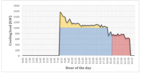
The energy audit highlights some opportunities to improve the cooling systems techno-economic performance. In particular, starting from the data presented in Figures 3.2 to 3.5, three area of intervention have been identified. Figure 3.7 shows the cooling load profile for a typical working day as measured over the 4 months monitoring period.
Figure 3.7: Cooling load profile for a normal operative day First area of intervention, Partial load operation (red area)
The audit showed that Chiller C has the highest rated COP (refer to Table 3.2); the datum is confirmed by the experimental data (refer to figure 3.6) which show
that the cooling system performs better (COP around 5.5) in the range of 1000-1100 kWc, whereas its performance decreases at partial load with COP dropping down to 4.9 at around 700 kWc. A possible intervention, hence, consists of exploiting storage technologies to avoid chiller partial load operations.
Second area of intervention, Peak-load management (yellow area)
At the present time, the BMS automatically manages the three chillers (refer to Table 3.1) to supply the exact quantity of cooling energy required. As already emphasized, the cooling system works most of the time in the maintaining phase supplying around 1000-1200 kWc of cooling energy which is very close to the 1050 kWc cooling capacity of chiller C ( refer table 3.1). Hence, a second possible area of intervention should address the opportunity of exploiting demand side management in order to reduce the peak load so that only the most performing chiller (chiller C, Table 3.1) is operated, with the two others serving as backup units.
Third area of intervention, Price arbitrage
This intervention is strictly economic and relates to the exploitation of the price arbitrage potential due to the difference between peak and off-peak electricity tariff in Singapore. The larger the spread between the peak and off-peak electricity tariff, the larger could be the economic benefit. In Singapore, the off-peak energy tariff is about 65% of the peak one. The peak period is between 07:00 and 23:00, which matches the daytime working schedule of the SADM building. Hence, the third area of intervention is to evaluate the techno-economic opportunity of shifting most of the cooling load from peak to off-peak hours.
The goal of this work is to assess the viability of using Cold Thermal Energy Storages (CTES) to implement demand side management strategies in order to in-crease the overall efficiency of the whole cooling system. In particular, the following actions are assessed:
3.3.2 Energy storage Modeling and design methodology
Energy Storage Model
For the techno-economic analysis, a deterministic model is adopted to simulate the behavior of the storage. The purpose of the model is to evaluate the amount of electrical energy consumed to charge the storage when in operation. The first step consists in defining the amount of cooling energy to be shifted by means of the storage depending on the type of action to be implemented. Once defined the amount of energy to be shifted, the amount of cooling Energy-To-Charge is
Figure 3.8: Energy storage model
calculated. The Energy-To-Charge can be easily calculated as:
ECharge=
EShif t
η (3.1)
Where is the charge/discharge efficiency of the storage, also called round trip efficiency. The storage efficiency is approximated as a constant parameter, evaluated considering the average charging, discharging and storing losses. The steady-state model does not account for the change in external conditions (e.g. temperature, humidity) which, in the real case, would affect the storage efficiency. This simplified model is particularly suited for a preliminary techno-economic feasibility study in Singapores climate characterized by almost steady ambient conditions along the day and across the year.
Cooling energy demand of the building
The assessment of the cooling energy demand of the building is essential for the techno-economic analysis of a CTES. Table 3.5 shows a list of parameters used to define the daily cooling energy demand of the building. For each month, the daily average cooling energy consumption of the building, the daily average COP (COPDA) of the chillers, the daily AVG electricity consumption (Daily AVG Elec-tricity Consumption) and the monthly cooling energy consumption (Monthly load) were calculated referring to the real load profiles, obtained by monitoring the cooling system for four months. In order to assess the effect of CTES on the performance of the cooling system, the COP of the system was also calculated for three different periods of the day: the Daily AVG COP, the Daily AVG COP between 07:00-18:00 and the Daily AVG COP between 19:00-23:00. Table 3.5 also reports the monthly surplus and the daily average surplus calculated from real acquired data. These values were calculated in order to address Action 2 (yellow area in Figure 3.7) in which only the most efficient chiller (chiller C) is operated during peak hours. The
Table 3.5: Cooling energy demand of the building Month Monthly load (kWhc) Daily AVG load (kWhc) Daily AVG elec load (kWhe) Daily AVG load 19-23 (kWhc) Daily AVG COP Daily AVG COP 19-23 Monthly sur-plus (kWhc) Daily AVG sur-plus (kWhc) March 344801 12771 2425 2714 5 5.2 4.3 9242 April 390061 14447 2744 2742 5.4 5.5 5.1 18273 May 359861 12409 2357 2547 5.3 5.4 5.1 6941 June 344000 11862 2253 2559 5.4 5.4 4.9 7332
Figure 3.9: Typical CTES system’s configuration
monthly surplus represents the sum of all the hourly surplus of a specific month. The daily average surplus is calculated as the Monthly Surplus divided by the num-ber of operative days. The hourly surplus (Esurplus) is defined as the difference between the hourly energy demand and the rated capacity of chiller C (CchillerC,i) and it is calculated for the ith hour as:
Esurplus,i= Edemand,i− CchillerC,i (3.2)
Storage technology and charge/discharge management
The medium considered in the CTES system is water (sensible heat storage) at atmospheric pressure operating with a temperature of 5°C (temperature range be-tween 7°C when fully charged and 12 °C when fully discharged). Figure 3.9 shows the proposed schematic diagram of the CTES.
The storage efficiency of the CTES system depends on its components such as the insulation material, the water diffusion mechanism inside the vessel, the auxiliary systems (pumps, heat exchanger). The thermal energy storage technology review
from Irena, indicates that TES systems have an efficiency which spans between 50% and 90% [108]. However, specific tests and experimental analysis carried out by some of the authors of this paper on a real sensible heat thermal energy storage located in Italy, have ascertained a storage efficiency of 85% [5]. The capital cost for the whole system was also calculated as 212 U S$/m3, including the cost for vessel, hydraulic system, compact heat exchanger and civil works. With regard to the operating strategies, TES system usually operates in full storage or partial storage mode. Full storage systems are designed to cover the whole energy demand during peak hours. On the contrary, partial storage systems shift the excess demand from a pre established threshold and can be used to shave the peaks, to stabilize the variable load of the energy demand or to partially replace the chillers system. CTES operating in full storage mode results in a larger and more expensive design since it aims to completely replace the cooling system during peak hours; this operating mode is usually suitable for large peak/off-peak spreads.
Comparison metrics
The main parameters utilized to assess costs and potential benefits of each proposed solution are the following: storage size, electricity to charge, percentage of electricity saved, economic savings, savings per energy unit (specific savings), estimated capital costs and payback period. The Storage size is calculated using the following relation:
Q = mcpδT (3.3)
Where Q represents the daily energy quantity to shift (based on the average working day and on the type of action addressed), expressed in kJ; m is the total mass of water stored in the vessel in kg; cp is specific heat of water at constant pressure, expressed in kJ/kgK; is the maximum temperature difference to which the storage medium is subjected. The Daily Electricity to Charge (kWh/day) represents the amount of electricity consumed to charge the storage. It is related to the Energy to Charge (Equation 3.1) and the chillers average COP during charge (COPcharge). As an example, when addressing the first area of intervention, the charge operations occurs during off-peak hours, with chillers operating at rated capacity and rated COP (see Table 3.1).
Echarge_daily =
Echarge
COPcharge
(3.4) The new Daily Electricity Consumption (Edaily_cons)after the CTES
introduc-tion is calculated according to Equaintroduc-tion 3.5, being a funcintroduc-tion of the Daily Electric-ity to Charge (Echarge_daily), the Daily Energy to Shift (Eshif t_daily) and the COP (COPphase) of the chillers in the phase considered (peak load, maintaining, partial load).
Edaily_cons= Edaily_con−
Eshif t_daily
COPphase
+ Echarge_daily (3.5) The performance of the chillers can be represented by the Daily AVG COP, either the Daily AVG COP 7-18 or the Daily AVG COP 19-23, depending on which portion of the energy demand is being shifted. As an example, when addressing the first area of intervention, shifting the energy to avoid partial load operations (red area, figure 3.7), the average COP considered is the Daily AVG COP 19-23. The Annual electricity savings (Savingsele), measured in kWh, are calculated as the difference between the Daily electricity consumption of the cooling system before and after the CTES introduction, multiplied by the Number of Operative Days per Year (Nd).
Savingsele= (Edaily_cons− Edaily_charge) ∗ N d (3.6) The Economic savings (Savingseco), measured in US dollars, are calculated as the difference between the yearly operative costs before and after the introduction of the energy storage. When evaluating the yearly operative costs the Energy-to-Shift per day, the Energy-To-Charge per day, the spread between peak (PT) and offpeak tariffs (OPT) and the number of operative days per year are taken into account.
Savingseco= (
Eshif t_daily
COPavg
− Edaily_charge)(P T − OP T ) ∗ N d (3.7) The Savings per energy unit (US$/kWhc) is obtained by dividing the economic savings by the energy capacity of the storage. This is a measure of the overall effectiveness of the solution. The Payback period (P BP ) (years) represents the main parameter to assess the economic feasibility of an investment: it is evaluated considering the capital costs (Capex) and the annual Economic savings.
P BP = Capex Savingseco