ON A GENERALISATION OF UNIFORM DISTRIBUTION AND
ITS PROPERTIES
K. Jayakumar
Department of Statistics, University of Calicut, Kerala - 673 635, India Kothamangalth Krishnan Sankaran1
Department of Statistics, S.N.College, Alathur, Kerala - 678 682, India
1. Introduction
Many researchers are interested in search that introduces new families of distri-butions or generalized some of the presented distridistri-butions which can be used to describe the lifetimes of some devices or to describe sets of real data. Exponential, Rayleigh, Weibull and linear failure rate are some of the important distributions widely used in reliability theory and survival analysis. However, these distri-butions have a limited range of applicability and cannot represent all situations found in application. For example, although the exponential distribution is often described as flexible, its hazard function is constant. The limitations of standard distributions often arouse the interest of researchers in finding new distributions by extending ones. The procedure of expanding a family of distributions for added flexibility or constructing covariates models is a well known technique in the lit-erature.
Uniform distribution is regarded to the simplest probability model and is related to all distributions by the fact that the cumulative distribution function, taken as a random variable, follows Uniform distribution over (0,1) and this result is basic to the inverse method of random variable generation. This distribution is also applied to determine power functions of tests of randomness. It is also applied in a power comparison of tests of non random clustering. There are also numer-ous applications in nonparametric inference, such as Kolmogrov-Smirnov test for goodness of fit. The uses of Uniform distribution to represent the distribution of roundoff errors and in connection with the probability integral transformations are also well known.
1.1. Marshall-Olkin family of distribution
Marshall and Olkin(1997) introduced a new family of distribution by adding a parameter to a family of distribution. They started with a survival function ¯F (x)
and considered a family of survival functions given by ¯
G(x) = α ¯F (x) F (x) + α ¯F (x).
Let X1, X2, ... be a sequence of independent and identically distributed random variables with survival function ¯F (x). Let N be a geometric random variable with
probability mass function P (N = n) = α(1− α)n−1, for n = 1,2,... and 0 <
α < 1. Then UN = min(X1, X2, ..., XN) has the survival function given by above
equation. If α > 1 and N is a geometric random variable with probability mass function P (N = n) = 1 α(1− 1 α) n−1, for n = 1,2,... then V N = max(X1, X2, ..., XN)
also has the survival function as above.
In the past, many authors have proposed various univariate distributions belonging to the family of Marshall-Olkin distributions. Also Jayakumar and Thomas (2008) proposed a new generalization of the family of Marshall-Olkin distribution as
¯ G(x; α, γ) = [ α ¯F (x) 1− (1 − α) ¯F (x) ]γ , f or α > 0, γ > 0, x∈ ℜ
1.2. Truncated Negative Binomial distribution
Nadarajah,et,al. (2013) introduced a new family of distributions as follows: Let X1, X2, ... be a sequence of independent and identically distributed random variables with survival function ¯F (x). Let N be a truncated negative binomial
random variable with parameters α∈ (0, 1) and θ > 0. That is,
P (N = n) = α θ 1− αθ ( θ + n− 1 θ− 1 ) (1− α)n f or n = 1, 2, ....
Consider UN = min(X1, X2, ..., XN). We have
¯ GUN(x) = αθ 1− αθ ∞ ∑ n=1 ( θ + n− 1 θ− 1 ) ((1− α) ¯F (x))n ¯ GUN(x) = αθ 1− αθ[(F (x) + α ¯F (x)) −θ− 1] (1) Similarly if α > 1 and N is a truncated negative binomial random variable with parameters 1
α and θ > 0, then VN = max(X1, X2, ..., XN) also has the survival
function given by (1). This implies that we can consider a new family of distribu-tions given by the survival function
¯
G(x; α, θ) = α
θ
1− αθ[(F (x) + α ¯F (x)) −θ− 1]
for α > 0, θ > 0 and x ∈ ℜ. Note that if α → 1 then ¯G(x; α, θ) → ¯F (x). The
family of distributions (1) is a generalization of the family of Marshall-Olkin dis-tributions. Namely, if θ = 1, then (1) reduces to the family of Marshall-Olkin distributions.
Suppose the failure times of a device are observed. Every time a failure occurs the device is repaired to resume function. Suppose also that the device is deemed no longer usable when a failure occurs that exceeds a certain level of severity. Let
X1, X2, ... denote the failure time and let N denote the number of failures. Then
UN will represent the time to the first failure of the device and VN will represent
the lifetime of the device. So (1) could be used to model both the time to the first failure and the lifetime.
In Section 2 we introduce the Generalised Uniform distribution and study its properties.Concluding remarks are presented in Section 3.
2. A new family of Uniform distribution
In this section, we set ¯F (x) = 1− x, 0 < x < 1 and introduce a new family of
distributions given by the survival function ¯
G(x; α, θ) = α
θ
1− αθ[[x(1− α) + α]
−θ− 1], θ > 0, α > 0. (2)
Therefore, the distribution function is given by
G(x; α, θ) =1− α
θ[x(1− α) + α]−θ
1− αθ (3)
The corresponding probability density function is given by
g(x; α, θ) = (1− α)θα
θ
(1− αθ)[x(1− α) + α]θ+1 (4)
for 0 < x < 1, α > 0, and θ > 0. We refer to this new distribution as the Gen-ralised Uniform distribution with parameters α and θ . We write it as GUD(α, θ). Remark I: If θ = 1, we obtain Marshall-Olkin Extended Uniform distribution in-troduced by Jose and Krsihna (2011).
Remark II: When θ = 1 and α→ 1, GUD reduces to standard Unifrom distribu-tion.
GUD(α, θ) random variable can be simulated using
X = ¯F−1
(
1− α[(1 − αθ)Y + αθ]−1θ
1− α
)
for Y ∼ Uniform (0,1). Therefore,
X = α 1− α ( [(1− αθ)Y + αθ]−1θ − 1 ) .
2.1. Shapes of the distribution and density function
If X follows GU D(α, θ), then
G(x; α, θ) =1− α
θ[x(1− α) + α]−θ
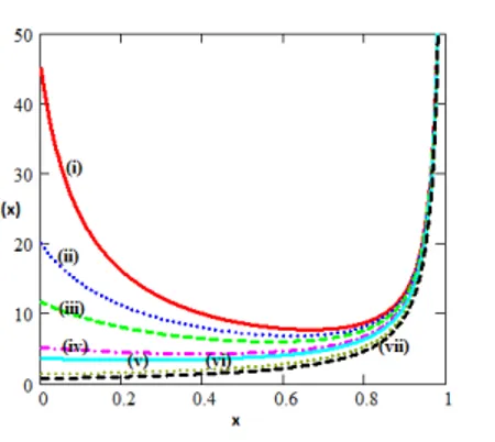
Figure 1 – The d.f of the GUD for different values of α when θ = 5 ;(i) α = 0.1 (ii)α = 0.5
(iii) α = 0.7 (iv) α = 0.9 (v) α = 1.1 (vi) α = 1.5 (vii) α = 1.9(viii) α = 5.
Figure 2 – The probability density function of the GUD for different values of α when θ = 5 (i) α = 0.1 (ii)α = 0.5 (iii) α = 0.7 (iv) α = 1.9(v) α = 5.
For different values of α when θ = 5, the structure of the distribution function is given in Figure 1.
In order to derive the shape properties of the probability density function, we consider the function
(log g)′= g ′(x) g(x) =− (1− α)(θ + 1) x(1− α) + α Let s(x) = (1x(1−α)(θ+1)−α)+α
i)If α ∈ (0, 1), then the function s(x) is positive and this implies that g is a decreasing function with g(0) = α(1(1−α)θ−αθ) and g(1) =
αθ(1−α)θ
1−αθ .
ii) If α > 1, then the function s(x) is negative and this implies that g is an increasing function with g(0) = α(α(α−1)θ−1) and g(1) =αθα(αθ−1−1)θ.
Some possible shapes of the probability density function g(x; α, 5) are given in Figure 2.
Figure 3 – The hazard function of the GUD for different values of α when θ = 5 (i) α = 0.1 (ii)α = 0.2 (iii) α = 0.3 (iv) α = 0.5 (v) α = 0.6 (vi) α = 0.9 (vii) α = 1.1
.
2.2. Hazard rate function
The hazard function of a random variable X with density g(x) and a cumulative distribution function G(x) is given by
h(x) = g(x)¯ G(x) =
θ(1− α)
[x(1− α) + α][1 − (x(1 − α) + α)θ]
Shapes of the hazard function h(x; α) for θ = 5 are presented in Figure 3. For α ≤ 0.6, hazard rate is initially decreasing and there exists an interval where it changes to be IFR. For α > 0.6, the hazard function is evidently IFR. Let us consider the reverse hazard rate function. The reverse hazard rate function is useful in constructing the information matrix and in estimating the survival function for censored data. The reverse hazard function of Generalised Uniform distribution is given by
r(x) = g(x) G(x) =
(1− α)θαθ
[x(1− α) + α][(x(1 − α) + α)θ− αθ]
The reverse hazard rate function decreases on (0, 1) with r(0)=∞ and r(1) = (1−α)θαθ
1−αθ .
2.3. Moments
If X has the GUD(α, θ) distribution, then the rthorder moment is given by
E(Xr) = ∫ 1 0 xr (1− α)θα θ (1− αθ)[x(1− α) + α]θ+1dx = (1− α)θα θ (1− αθ) ∫ 1 0 xr [x(1− α) + α]θ+1dx.
By equation 2.2.5.2 Prudinikov et,al. (1986), ∫ b a (x− a)(α−1) (cx + d)α+n+1dx = (b− a)α (ac + d)(bc + d)α n ∑ k=0 ( n k ) B(α + k, n− k + 1) (bc + d)k(ac + d)n−k
where B(a, b) = Γ(a+b)ΓaΓb
E(Xr) = (1− α)θα θ) α(1− αθ θ−r−1∑ k=0 ( θ− r − 1 k ) B(r + k + 1, θ− r − k) αn−k = (1− α)θα θ−1 (1− αθ) θ−r−1∑ k=0 ( θ− r − 1 k ) Γ(r + k + 1)Γ(θ− r − k) Γ(θ + 1)αn−k . (5)
Using (5), we get the mean and the variance of a random variable X with GU D(α, θ) are respectively as µ′1 = αθ 1− αθ [ α(1 + α−θ) + θ(1− α) (1− α)(1 − θ) ] , and µ2 = α θ (1−αθ) [ −1 + 2( 1 (1−α)(1−θ)− (1−α−θ+2) (1−α)2(1−θ)(2−θ) ) − αθ 1−αθ ( α(1+α−θ)+θ(1−α) (1−α)(1−θ) )2] .
The qthquantile of a random variable X with GU D(α, θ) is given by
xq = G−1(q) = α 1− α [ 1 [1− q(1 − α)θ]1θ − 1 ] , 0≤ q ≤ 1,
where G−1(.) is the inverse distribution function. In particular, the median of
GU D(α, θ) is given by M edian(X) = α 1− α [ 1 [1−12(1− α)θ]1θ − 1 ] . 2.4. Order Statistics
Assume X1, X2, ..., Xn are independent random variables having the GU D(α, θ)
distribution. Let Xi:n denote the ithorder statistic. The probability density
func-tion of Xi:n is gi:n(x; α, θ) = n! (i− 1)!(n − 1)!g(x; α, θ)G i−1(x; α, θ) ¯Gn−i(x; α, θ) = n! (i− 1)!(n − i)! [ (1− α)θαθ (1− αθ)[x(1− α) + α]θ+1 ] [ 1− α θ (1− αθ)[(x(1− α) + α) −θ− 1]] i−1 [ αθ (1− αθ)[(x(1− α) + α) −θ− 1]] n−i .
2.5. Renyi and Shannon entropies
An entropy is a measure of variation or uncertainty. The Renyi entropy of a random variable with probability density function g(.) is defined as
IR(γ) = 1 1− γlog ∫ ∞ 0 gγ(x)dx, γ > 0, γ ̸= 1.
The Shannon entropy of a random variable X is defined by E[-log g(X)]. It is a particular case of the Renyi entropy for γ↑ 1. We have
∫ ∞ 0 gγ(x)dx = ∫ 1 0 [ (1− α)θαθ (1− αθ)(x(1− α) + α)θ+1 ]γ dx = [ (1− α)θαθ 1− αθ ]γ[ αγ(θ+1)+1− 1 (1− γ(θ + 1))(1 − α)αγ(θ+1)+1 ] So the Renyi entropy is
IR(γ) = 1 1− γlog ([ (1− α)θαθ 1− αθ ]γ[ αγ(θ+1)+1− 1 (1− γ(θ + 1))(1 − α)αγ(θ+1)+1 ]) Now consider the Shannon entropy. From its definition, we have
E[−log g(X)] = E [ log 1− α θ (1− α)θαθ + (θ + 1)log[x(1− α) + α)] ] = log 1− α θ (1− α)θαθ + (θ + 1)E(log[x(1− α) + α]) E(log[X(1− α) + α]) = (1− α)θα θ 1− αθ ∫ 1 0 log[x(1− α) + α] [x(1− α) + α]θ+1dx = θα θ 1− αθ [ α−θlogα + (α −θ− 1) θ2 ] Hence E[−log g(X)] = log 1− α θ (1− α)θαθ + θ(θ + 1)αθ 1− αθ [ α−θlogα +(α −θ− 1) θ2 ] 2.6. Estimation
Since the moments of an GUD random variable cannot be obtained in closed form, we consider estimation of the unknown parameters by the method of maximum likelihood. For a given sample (x1, x2, ..., xn), the log-likelihood function is given
by log L(x; α, θ) = nlog(1− α)θα θ 1− αθ + n ∑ i=1 log 1 [xi(1− α) + α]θ+1
= nlog(1− α) + nlogθ + nθlogα − nlog(1 − αθ)
−(θ + 1)
n
∑
i=1
The partial derivatives of the log likelihood function with respect to the parameters are ∂logL ∂α = −n 1− α+ nθ α + nθαθ−1 1− αθ − (θ + 1) n ∑ i=1 (1− xi) [xi(1− α) + α] , ∂logL ∂θ = n θ + nlogα 1− αθ − n ∑ i=1 log[xi(1− α) + α].
The maximum likelihood estimates can be obtained numerically solving the equa-tion ∂logL∂α = 0 and ∂logL∂θ = 0. We can use, for example, the function nlm from the programming language R.
The second derivatives of the log likelihood function of GUD with respect to
α and θ are given by ∂2logL ∂α2 = n (1− α)2 − nθ α2 + nθαθ−2(1 + θ− αθ) (1− αθ)2 + (θ + 1) n ∑ i=1 (1− xi)2 [xi(1− α) + α]2 , ∂2logL ∂θ2 = −n θ2 + nαθlog2α (1− α2)2, ∂2logL ∂θ∂α = n α+ nαθ−1(1− αθ) + nθ(θ− 1)αθ−2(1− α)θ+ nθ2α2(θ−1) (1− αθ)2 − n ∑ i=1 (1− xi) [xi(1− α) + α] .
If we denote the MLE of β = (α, θ) by ˆβ = ( ˆα, ˆθ), then the observed information
matrix is given by I(β) = −E ∂2logL ∂α2 ∂2logL ∂θ∂α ∂2logL ∂θ∂α ∂2logL ∂θ2
and hence the variance covariance matrix would be I−1(β). The approximate (1− δ)100% confidence intervals for the parameters α and θ are ˆα ± Zδ
2 √ V ( ˆα) and ˆθ± Zδ 2 √
V (ˆθ) respectively, where V ( ˆα) and V (ˆθ) are the variances of ˆα and
ˆ
θ, which are given by the diagonal elements of I−1(β), and Zδ
2 is the upper ( δ
2) percentile of standard normal distribution.
3. Conclusion
In this paper, we have introduced and studied a new family of distribution con-taining the Uniform as a generalization of the Marshall-Olkin extended uniform distribution studied in Jose and Krishna(2011). As a data analysis point of view GUD are more feasible and tractable. We have derived some properties of the Generalised Uniform distribution such as probability density function, hazard rate
function , moments, distribution of order statistics, Renyi entropy and Shannon entropy. Estimation of parameters is done using maximum likelihood.
References
K. Jayakumar, M. Thomas (2008). On a generalization to Marshall-Olkin
scheme and its application to Burr type XII distribution. Statist. Pap., 49,
421-439.
K. K. Jose, E. Krishna (2011). Marshall-Olkin extended uniform distribution. ProbStat Forum, 04, 78-88.
A. W. Marshall, I. Olkin (1997). A new method for adding a parameter to a
family of distributions with application to the exponential and Weibull families.
Biometrika, 84, 641-652.
S. Nadarajah, K. Jayakumar, M. M. Ristic (2013). A new family of lifetime
models. Journal of Statistical Computation and Simulation, 83, 1389-1404.
A. P. Prudnikov, Y. A. Brychkov, O. I. Marichev (1986). Integrals and
series vol. I. Gordeon and Breach Sciences, Amsterdam, Netherlands.
Summary
Nadarajah et al.(2013) introduced a family life time models using truncated negative binomial distribution and derived some properties of the family of distributions. It is a generalization of Marshall-Olkin family of distributions. In this paper, we introduce Generalized Uniform Distribution (GUD) using the approach of Nadarajah et al.(2013). The shape properties of density function and hazard function are discussed. The expres-sion for moments, order statistics, entropies are obtained. Estimation procedure is also discussed.The GDU introduced here is a generalization of the Marshall-Olkin extended uniform distribution studied in Jose and Krishna(2011).
Keywords: Distribution of order statistics; Entropy; Marshall-Olkin family of
distribu-tions; Maximum likelihood; Random variate generation; Truncated negative binomial distribution.