Machine Learning Aided Methods for Resilient Industrial Wireless Sensor Network

ALMA MATER STUDIORUM

UNIVERSITÁ DI BOLOGNA

SCUOLA DI INGEGNERIA E ARCHITETTURA

Corso di Laurea Magistrale in Ingegneria Informatica

TESI DI LAUREA MAGISTRALE

in

Embedded System

Machine Learning Aided Methods for

Resilient Industrial Wireless Sensor Network

Candidato: Relatore:

Andrea Bombino

Stefano Mattoccia

Correlatore: Prof.

Mikael Gidlund

Simone Grimaldi

Aamir Mahmood

Anno Accademico 2017/2018

Sessione III

Abstract

A Wireless Sensor Network (WSN) is an infrastructure comprised of sens-ing, computsens-ing, and communication devices, that obtains and processes data to understand the behavior of the monitored environment, and to react to events and phenomena that occur within that. The use of WSN in industry settings is extremely appealing, nevertheless most industrial environments are obstile to reliable radio communication, showing pronounced effects of multipath fading, strong attenuation and radio interference. This motivates a huge effort in research activities, standardization process and industrial investments on this field since the last decade. In our work, we propose mechanisms based on machine learning algorithms that allows us to classify the channel propagation condition (Line-of-Sight and Non-Line-of-Sight) of radio links. The investigated methods provide an useful diagnostic tool in the context of adaptive transmission strategies for improving the quality and reliability of wireless communication.

In particular, the first mechanism is based on the analysis of I/Q data, while the second method is based on bit-error pattern distribution in re-ceived packets. Both the solutions have been implemented on real hardware and tested in a number of environment with heterogeneous characteristics, showing promising results.

Prefazione

Una Wireless Sensor Network (WSN) può essere definita come un’ infras-truttura composta da sensori/dispositivi in grado di calcolare, comunicare e effettuare sensing dell’ambiente circostante processando e analizzando i dati in modo da reagire a eventi e fenomeni che possono occorrere durante la comunicazione. L’utilizzo delle WSN nel settore industriale è estremamente allettante, nonostante la maggior parte du questi ambienti risulti ostile alle comunicazioni radio affidabili, mostrando effetti sensibili di cammini multi-pli, forte attenuazione e interferenze radio. Questo motiva un enorme effort nella ricerca, standardizzazione e investimento industriale in questo campo, nell’ultimo decennio. L’uso delle WSN nell’ambiente industriale è soggetto a diverse problematiche, dovuto all’ostilità del canale radio in ambito indus-triale, come rumore, Shadwoing, cammini multipli e interferenze. Nel nostro progetto, proponiamo meccanismi basati sulle condizioni di propagazione del canale e algoritmi di machine learning che ci permettono di classificare lo stato del canale (Line-of-Sight o Non-Line-of-Sight). I metodi analizzati for-niscono un utile strumento diagnostico nel contesto delle strategie di trasmis-sione adattiva per migliorare la qualità e l’affidabilità della comunicazione wireles.

In particolare, il primo meccanimo è basato sull’analisi degli I/Q data, mentre il secondo metodo è basato sull’analisi della distribuzione del bit-error pattern nel pacchetto ricevuto. Entrambe le soluzione sono state implemen-tate su hardware e tesimplemen-tate in differenti ambienti con differenti caratteristiche, mostrando risulati promettenti.

Contents

1 Introduction 5

1.1 Motivation . . . 5

1.2 An Overview on Availaible Approaches . . . 6

1.3 Problem Statement . . . 6

1.4 Thesis Contribution . . . 7

1.5 Thesis Outline . . . 7

2 Background 9 2.1 Wireless Sensor Network . . . 9

2.1.1 Architecture . . . 10

2.1.2 Network Topologies . . . 11

2.2 Industrial Wireless Sensor Network . . . 12

2.2.1 IWSN Requirements . . . 12

2.2.2 IEEE 802.15.4 . . . 14

2.2.3 RF Interference . . . 16

2.2.4 Multipath Fading . . . 19

2.2.5 Slow and Fast Fading . . . 20

2.2.6 Rayleigh Distribution . . . 22 2.2.7 Rice Distribution . . . 24 2.3 Signal Representation . . . 25 2.3.1 I/Q Data . . . 25 2.4 Cognitive Radio . . . 30 2.5 Machine Learning . . . 31 2.5.1 Unsupervised Learning . . . 32

2.5.2 Supervised Learning . . . 32

3 Related Work 37 4 Radio Link Characterization 39 4.1 Intuition . . . 39

4.2 Classification of the Radio-Link State . . . 40

4.2.1 Data Analysis . . . 41 4.2.2 Classification Model . . . 43 5 Experimental Set-up 47 5.1 LabVIEW . . . 47 5.1.1 USRP . . . 48 5.2 Development Libraries . . . 49 5.2.1 Scikit-Learn . . . 49 5.2.2 Keras . . . 50 5.3 Software Design . . . 50

5.3.1 Data Collection and Preparation . . . 51

5.3.2 Real-time Classification . . . 53

6 Experiments 55 6.1 Industrial Environment Dataset - Imerys Mineral AB . . . 55

6.2 Lab Environment Dataset . . . 57

6.3 Mixed Dataset . . . 59

6.4 Semi-industrial Environment - Mechanical Workshop . . . 60

6.5 Discussion . . . 62

6.5.1 Features Separation . . . 62

6.5.2 Bit Error Pattern Approach . . . 63

7 Conclusion 67 7.1 Future Work . . . 67

Acronyms

The following list represents the acronyms used in the thesis.

BEP Bit Error Pattern

BPSK Binary Phase Shift Keying DSSS Direct Sequence Spread Spectrum FHSS Frequency Hopping Spread Spectrum ISM Industry Science Medical

LOS Line-of-Sight

MAC Media Access Control NLOS Non-Line-of-Sight NN Neural Network

OQPSK Offset Quadrature Phase Shift Keying PDF Probability Density Function

PHY Physical Layer QoS Quality of Service RF Radio Frequency

RSSI Received Signal Strength Indicator SDR Software Defined Radio

TSCH Time-slotted Channel Hopping USRP Universal Software Radio Peripheral WLAN Wireless Local Area Network WSN Wireless Sensor Network

Chapter 1

Introduction

Since the beginning of the third Millennium, Wireless Sensor Networks (WSNs) have generated an increasing interest from industrial and research perspec-tives [1]. A wireless sensor network can be generally described as a multi-hop self-organizing network composed of multiple sensor devices, which commu-nicate with each other wirelessly. It is composed of many sensor nodes with the ability to sense and the possibility to control the environment enabling interaction between persons or computers and the surrounding environment, collecting and processing information. They have resource constraints, with low processing power and, in some cases, restrictions in power consumption.

1.1

Motivation

The use of WSN in industrial systems presents some challenges[2]. Wireless networks use an inherently unreliable communication medium which can be aggravated due to noise and interference in the spectrum band used for com-munication. The majority of wireless sensor networks work in the 2.4 GHz unlicensed frequency band, reserved for Industrial, Scientific and Medical (ISM) applications. This means that the WSN have to deal with unwanted RF interference, in addition to the typical adverse effects of multipath fading and signal attenuation. The WSN can be used in domains such as

agri-In the industry environment, the characteristics of the wireless channel are different in comparison to other WSN environments, such as home and of-fice environments. The sensors are deployed to monitor critical parameters such as vibration, temperature, pressure and motor efficiency. In addition, the wireless channel in many industrial environments is non-stationary on a long time-scale, which can cause abrupt changes in the characteristics of the channel over time. These shortcomings can seriously affect the communica-tion link quality of Wireless Sensor Networks. A set of standards, such as WirelessHART, ISA100.11a, was developed for industrial WSN to partially overcome these limitations.

1.2

An Overview on Availaible Approaches

In the related literature, it is possible to find a number of works targeting the topic of radio-link state estimation in WSN. A common approach for the physical layer measurement is to rely on the Received Signal Strength Indicator (RSSI) values provided by the chipset. Because, the measuraments and calculation involved with RSSI are less complicated, and RSSI values are easily available [3]. Anyway, the RSSI data analysis present some drawbacks due to the low-resolution of the RSSI data available on most WSN plat-tforms. Therefore, as the computation could be more heavy the I/Q data analysis give us more information about the channel properties and studying the distribution, by means of theoretical model like Rician and Rayleigh dis-tribution [4], so that it is possiblie, it is possible to infer the signal properties. On top of this, machine learning methods are built and trained to classify the radio link propagation-state both offline and online way, with a variable level of complexity and performance.

1.3

Problem Statement

In this thesis, we focus on the radio link state. In particular, we want to distinguish between Line-of-Sight (LOS) and No-line-of-Sight (NLOS)

conditions. Starting with the analysis of received signals, our goals are an-alyze, detect and classify the sources of link disruption during the packet transmission using two approaches: first, based on I/Q data analysis and the second, based on analyzing the Bit Error Pattern distribution [5].

1.4

Thesis Contribution

Although, as mentioned in Section 1.2, there are independent efforts in the literature on these topics, we envision the development of a unified frame-work for channel state detection and classification frameframe-work that moves beyond the existing approaches by incorporating link quality prediction and link/network adaption in the framework. To this end, we use machine learn-ing tools along with the spectrum senslearn-ing, signal processlearn-ing and wireless communication principles to enhance the resilience of industrial WSNs. For this purpose, we introduce the classification procedure; combining the results of signals analysis methods [3] and [6] to categorize the radio channel state. We use a Software Defined Radio as transceiver and receiver. Capturing sig-nal with SDR gives us possibility to asig-nalyze the statistical properties of the received signal, enabling the use of various machine learning method.

1.5

Thesis Outline

The rest of the thesis is organized as follows. In Chapter 2 we give a de-scription of wireless sensor networks, in particular industrial wireless sensor networks and their main challenges. We also provide a brief description of machine learning solutions with specific interest to supervised learning-based methods. We then explore other related works about this topic in Chapter 3. Then, we describe in detail the Radio Link Sate in Chapter 4, focusing in particular on the techniques to model the issue. In Chapter 5 we elaborate the problem and how we tackle it. The experiments results on real datasets are discussed in Chapter 6. The thesis is concluded with Chapter 7 where future work is discussed as well.

Chapter 2

Background

In this chapter we introduce the fundamental concepts within the scope of this thesis. We begin by describing the wireless sensor network and the main techniques to address the problems. We then outline a number of machine learning techniques commonly used in signal processing.

2.1

Wireless Sensor Network

A WSN is a network formed by a large number of sensor nodes where each node is equipped with a sensor to detect physical phenomena such as light, heat, pressure. WSNs are regarded as a revolutionary information gather-ing method to build the information and communication system which will greatly improve the reliability and efficiency of infrastructure systems. Com-pared with the wired solution, WSNs feature easier deployment and better flexibility of devices. The main features of WSNs are: scalability with respect to the number of nodes in the network, self-organization, self-healing, energy efficiency, a sufficient degree of connectivity among nodes, low-complexity, low cost and size of nodes. With the rapid technological development of

History

Research on WSNs dates back to the early 1980s when the United States Defense Advanced Research Projects Agency (DARPA) carried out the dis-tributed sensor networks (DSNs) programme for the US military [7].

At that time, the Advanced Research Projects Agency Network (ARPANET) had been in operation for a number of years, with about 200 hosts at uni-versities and research institutes. DSNs were assumed to have many spatially distributed low-cost sensing nodes, collaborating with each other but oper-ated autonomously, with information being routed to whichever node not that can use the Information most effectively. Even though early researchers on sensor networks had the vision of a DSN in mind, the technology was not quite ready. The sensors were rather large (i.e. the size of a shoe box and bigger), and the number of potential applications was thus limited. As related technologies mature, the cost of WSN equipment has dropped dra-matically, and their applications are gradually expanding from the military areas to the industrial and commercial field.

2.1.1

Architecture

Modern WSN usually include sensor nodes, actuator nodes, gateways and clients. A number of sensor nodes is deployed in the designed area with the scope of monitoring certain physical properties of the environment. The nodes can be organized in star or mesh topologies, while the WSN protocols usually provide self-organizing capabilities by means of multi-hopping com-munication.

The sensor node is one of the main parts of a WSN. The hardware of a sensor node generally includes four parts: the power and power management module, a sensor, a micro-controller, and a wireless transceiver. A sensor is in charge of collecting and transforming the signals, such as light, vibration and chemical signals into electrical signals and then transferring them to the micro-controller. The micro-controller receives the data from the sensor and processes them accordingly.

2.1.2

Network Topologies

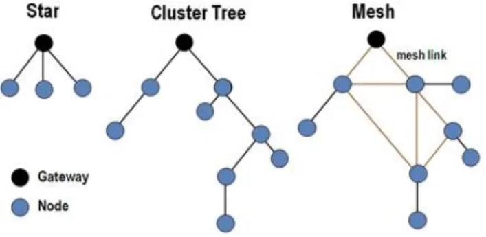
WSN nodes are typically organized in one of three types of network topolo-gies:

Figure 2.1: WSN topologies

1. Star: In a star topology, each node connects directly to a gateway. A single gateway can send messages to as well as receive them from a number of remote nodes. The nodes are not permitted to send messages to each other, which allows low-latency communications between the remote node and the gateway (base station).

2. Cluster Tree: It is also called as cascaded star topology. In cluster tree topologies, each node connects to a node that is placed higher in the tree and then to the gateway. The main advantage of the cluster tree topology is that the expansion of a network can be easily done. 3. Mesh: It allows transmission of data from one node to another, within

its radio transmission range. If a node wants to send a message to a node located out of its radio communication range, it needs an inter-mediate node to forward the message to the desired node.

2.2

Industrial Wireless Sensor Network

The indoor radio channel has active area of research [8]. Due to increasing use of indoor wireless communications. While wireless communication standards, such as IEEE 802.11, are already largely adopted in office environments for non-critical applications, during the last few years many manufacturing com-panies have been interested to incorporate wireless communication in their production processes. This implies a certain number of technical challenges due to the highly dynamic changes of the workplace layout overtime, the presence of machinery and highly reflective materials. Hence, the use of WSN in these environments, is subject to typical problems of wireless com-munications, such as noise, shadowing and multipath fading. The lack of reliability makes it difficult to provide Quality of Service (QoS) guarantees. The characterization of the industrial environments with respect to inter-ference sources and propagation characteristics, is an important step in the development reliable wireless networks and to improve the current IWSN standard, namely WirelessHART, ISA100.11a, WISA, ZigBee [9]. All the aforementioned standards are based on the IEEE 802.15.4 physical layer, but have defined different mechanisms for the upper layers. In addition, we also mention IWLAN [9] that is based on the IEEE 802.11.

2.2.1

IWSN Requirements

Simple deployment, significant cost savings in installations, lack of cabling, high mobility, easy rearrangements related to device configuration and sensor locations make the wireless network technologies also appealing for industrial application. The adaption of wireless technologies appealing in industrial environment possesses additional challenges since the factory environments are typically harsh for wireless communication in terms of interferences, noise and physical obstacles. The following list includes some of the common requirements found in industrial applications:

• Standardized Solutions: In order to provide flexibility and freedom to choose among a broad set of suppliers with guaranteed

interoper-ability, standardized and open communication protocols should be used instead of specific proprietary protocols. Besides facilitating repair-ment and replacerepair-ment procedures in case of equiprepair-ment faults, the use of standardized solutions usually extends the lifespan of the network, since there is not a direct dependence on a specific vendor success or failure.

• Reliable Performance: For most applications, it is desirable to have network reliability close to 100%. In other words, the sensor data loss should be minimal. Employing redundant paths, self-healing algo-rithms, and retransmission schemes are some example of possible ways through which highly reliable performance can be achieved, even under the harsh and rapidly changing conditions that characterize industrial environments.

• Energy efficiency: In wireless systems, the power needed to feed the devices must come from local sources, normally small batteries. For this reason, efficient energy consumption is a greatly desired quality and wireless sensors must be able to provide a battery life of several months and even years. Considering that self-organizing and self-healing pro-cedures, as well as the data relay, demand different energy levels, it can be said that power consumption is a non-deterministic metric. Energy harvesting from thermal sources, for instance, is one of the most used options to extend the battery life of nodes.

• Friendly coexistence: Most wireless technologies operate in the 2.4 GHz ISM frequency band. To enable the deployment of IWSN and Wireless Local Area Networks (WLAN) in the same facilities, which is a remarkably relevant scenario, the involved technologies must be able to coexist without degradation in their performances. The implemen-tation of an opportune frequency channel mapping, channel sensing techniques and the use of frequency hopping algorithms, are some of the widely used solutions to avoid or reduce interference.

• Operation in Harsh Environments: Environmental conditions that an IWSN may encounter are strongly dependent on the specific location in which it is deployed. Hence, operational temperatures, humidity, noise and hazard characteristics will greatly vary from case to case. Before deploying a network in a plant, strict verification should be performed to ensure that the equipment used is capable of withstanding the given conditions and, more importantly, if it complies with the legal regulations of the country.

2.2.2

IEEE 802.15.4

The Institute of Electrical and Electronics Engineers (IEEE) supports many working groups to develop and maintain wireless and wired communications standards. For example, 802.3 is wired Ethernet and 802.11 is for wire-less LANs (WLANs), also known as Wi-Fi. The 802.15 group of standards specifies a variety of wireless personal area networks (WPANs) for different applications. For instance, 802.15.1 is Bluetooth, 802.15.3 is a high-data-rate category for ultra-wideband (UWB) technologies, and 802.15.6 is for body area networks (BAN). There are several others [10]. The 802.15.4 standard defines the physical layer (PHY) and media access control (MAC) layer of the Open Systems Interconnection (OSI) model of network operation. The PHY defines frequency, power, modulation, and other wireless conditions of the link. The MAC defines the format of the data handling. The remaining layers define other measures for handing the data and related protocol en-hancements including the final application. The goal of the standard is to provide a base format to which other protocols and features could be added by way of the upper layers. While three frequency assignments are available, the 2.4-GHz band is by far the most widely used 2.1. Most available chips and modules use this popular ISM band.

Several society, such as ISA, have been actively pushing the applications of wireless technologies in industrial automation [11]. Moreover different standard are realized like ZigBee, WirelessHart and ISA100 that use the same physical layer of IEEE 802.15.4, but they differ substantially concerning the medium access control level (MAC) [10], [9].

ZigBee

ZigBee is a standard containing a suite of protocols using low-power ra-dio based on the IEEE 802.15.4 standard. Mesh network configuration of ZigBee[11] is considered to be a cost-effective solution for the use in different industrial applications. The nodes consume low energy and support different topologies. The standard uses the 868 MHz band in Europe, 915 MHz in the United States, and 2.4 GHz globally. Offset Quadrature Phase Shift Keying (OQPSK) modulation is used at 2.4 GHz, whereas binary phase shift key-ing (BPSK) modulation is used for the 868 MHz and 915 MHz. Generally, ZigBee targets applications that require low data rate and long battery life, making it a good candidate for wireless sensor and control applications. In order to increase the IEEE 802.15.4 network lifetime, the nodes are usually required to transmitt at a low power level. This makes them more vulnerable to noise, interference, and multipath distortion.

WirelessHart

WirelessHart is a sensor network technology based on the highway address-able remote transducer (HART) protocol. It uses the 802.15.4 standard with O-QPSK modulation at 2.4 GHz achieving a data rate of up to 250 kb/s. Di-rect sequence spread spectrum [9] (DSSS) is used together with a time-slotted channel hopping (TSCH) technique [9] to mitigate the effect on interference and multipath distortion on packet-by-packet basis. Unlike WirelessHART [11], ZigBee systems uses the same static channel and are thus more suscep-tible to noise, interference, and multipath effects.This makes WirelessHart more robust than ZigBee for deployment in harsh industrial environments.

In addition to DSSS and TSCH, link-level acknowledgment (ACK) for package re-transmission, graphic routing for path diversity, and transport protocol with end-to-end acknowledgments are used to achieve reliable data transmission.

ISA100

This standard for industrial automation and control applications was devel-oped by the International Society of Automation (ISA). The ISA100 physical layer is based on the IEEE 802.15.4 standard at 2.4 GHz with DSSS and FHSS, providing a data rate of up to 250 kb/s. The main difference be-tween ISA100 and WirelessHART is the main goals of each standard. While WirelessHART is designed to address issues such as reliability, security and interoperability. In general, ISA100 is designed to have broad coverage of in-dustrial automation networks and aims to converge/assimilate existing net-works using different communication protocols.

2.2.3

RF Interference

As mentioned previously, industrial applications have higher QoS require-ments than typically found in homes and offices. More communication de-vices are involved and their number is variable. It is necessary to meet specific safety and security requirements, and performance must be deter-ministic with certain degradation. Coupled with the harsh environment, this means that the spectrum resources vary over time and space. This situa-tion may be exacerbated by device mobility and traffic fluctuasitua-tions. When different radio signals exist in the same place, at the same time and in a common frequency range, then Radio Frequnecy Interference (RFI) occurs[9]. This is particularly a problem when using devices that operate in the ISM and Unlicensed National Information Infrastructure (U-NI) bands, which are both unlicensed and used for different networks including Wireless Personal Area Networks (WPANs), such as WSN, and Wireless Local Area Networks (WLANs). This can be exacerbated by poor frequency planning and a overly crowded frequency spectrum. WirelessHART, ISA 100.11.a, ZigBee, Wi-Fi,

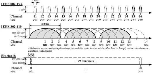
Bluetooth device operates in the 2.4 GHz ISM band, as do other devices. The following table [9] gives a comparison of different industrial wireless platforms that need to coexist.

IWLAN ZigBee WirelessHart ISA 100.11a WISA

Bandwidth 22 MHz 2 MHz 2 MHz 2 MHz 1 MHz

Channels. Selection 14, static 16, static 15, dynamic 15, dynamic 15, dynamic

Data Rate 11-54 Mps 250 kps 250 kps 250 kps 1 Mps

Frequency Band(s) 2.4 GHz, 5 GHz 2.4 GHz 2.4 GHz 2.4 GHz 2.4 GHz MAC Layer IEEE 802.11 IEEE 802.15.4 Proprietary Proprietary Proprietary Radio IEEE 802.11b/g/a IEEE 802.15.4 IEEE 802.15.4 IEEE 802.15.4 IEEE 802.15.1

Table 2.1: Wireless Industrial Standards

The effect of the interference in these coexistence standard could also be seen in the channel overlapping as shown in the following figure 2.2.

Figure 2.2: Overlapping of IEEE 802.15.4 and IEEE 802.11b and Bluethooth channel allocation

IEEE 802.11

IEEE 802.11 is a family of progressively improved wireless local area network (WLAN) standards [11]. In 1999, the IEEE 802.11b standard was published to operate in the unlicensed 2.4 GHz band with a maximum transmission rate of 11 Mb/s. IEEE 802.11a was released later in the same year to support up to 54 Mb/s in the 5 GHz frequency band. Further enhancements of the standard, IEEE 802.11g, allowed the same rates (54 Mb/s) to be obtained in the 2.4 GHz band, while traffic differentiation mechanisms, were introduced in a subsequent amendment, referred as IEEE 802.11e. Several important improvements were further introduced in IEEE 802.11n to support multiple-input multiple-output (MIMO) and channel bonding capabilities to increase the reliability, coverage, and transmission rate (up to 6000 Mb/s).

The above discussed IEEE 802.11 family of standards have been consid-ered for the use in various industrial applications. However, one of the main challenges of these systems is the issue of interference.

In the 2.4 GHz band, three non-overlapping channels are used to create a cellular architecture, which is not enough to sufficiently isolate micro-cells on the same channel. A significant amount of system capacity is thus lost to co-channel interference. IEEE 802.11n reduces the interference by utilizing more channels in the 5 GHz band, but cannot entirely eliminate the issue. The use of antenna beamforming in IEEE 802.11n dramatically increases the range but also leads to increased interference over distance. Although the IEEE 802.11 family of standards can provide relatively high data rates, the issue of interference will continue to be a key challenge in designing robust highly reliable industrial wireless networks. In addition, the reduction in performance of these systems with regard to the propagation characteristics of harsh industrial environments could be significant.

2.2.4

Multipath Fading

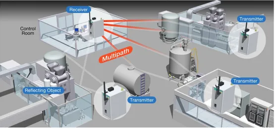
Compared to other indoor and outdoor, the industrial radio channel is usually harsher with respect to radio propagation. In addition, the wireless chan-nel in many industries is non-stationary in the long term, which can cause abrupt changes in the characteristics of the channel over time. Common characteristics of these environments are affecting by large-scale and small-sale fading causing multipath. Multipath is the propagation phenomenon that results in radio signals reaching the receiving antenna from two or more paths. The effects of multipath include constructive and destructive inter-ference, phase shifting of the signal cause errors and impact of the quality of the communications.

Fading

The term fading refers to rapid fluctuations of the amplitude, phase of a radio signal over a short period o short travel distance.

In principle, the following are the main multipath effects:

1. Rapid changes in signal strength over a small travel distance or time interval.

2. Random frequency modulation due to varying Doppler shifts on differ-ent multipath signals.

3. Time dispersion or echoes by multipath propagation delays.

In wireless communications, the presence of reflectors in the environment surrounding a transmitter and receiver create multiple paths that a trans-mitted signal can traverse. As a result, the receiver sees the superposition of multiple copies of the transmitted signal, each traversing a different path. Each signal copy will experienced differences in attenuation, delay and phase shift while travelling from the source to the receiver. This can result in either constructive or destructive interference, amplifying or attenuating the signal power seen at the receiver.

Thus, in communication it could produce several problems: • Inter-symbolic Interference

• Large fluctuation of received power

These drawbacks bring errors in receiving symbols.

Figure 2.3: Multi-path fading in Wireless Communication

2.2.5

Slow and Fast Fading

Mathematically, fading is usually modeled as a time-varying random change in the amplitude and phase of the transmitted signal [4]. The terms slow and fast fading refer to the rate at which the magnitude and phase change imposed by the channel on the signal changes. The coherence time is a measure of the minimum time required for the magnitude change of the channel to become decorrelated from its previous value.

• Slow Fading: Slow fading arises when the coherence time of the channel is large relative to the delay constraint of the channel. In this regime, the amplitude and phase change imposed by the channel can be considered roughly constant over the period of use. Slow fading can be caused by events such as shadowing, where a large obstruction such as a hill or large building obscures the main signal path between the

transmitter and the receiver. The amplitude change caused by shad-owing is often modeled using a log-normal distribution with a standard deviation according to the Log Distance Path Loss Model.

P L = PT + GT + GR− LT − LR− PR (2.1)

In 2.1:

– PT: is de transmitter power in dBm.

– GT and GR: are the Tx and Rx antenna gain in dBi.

– LT and LR: are the antenna cable losses in dB.

– PR: is the local mean received power.

• Fast Fading: : Fast fading occurs when the coherence time of the channel is small relative to the delay constraint of the channel. In this regime, the amplitude and phase change imposed by the channel varies considerably over the period of use.

Temporal Fading

Temporal fading is defined as the variability of the received power over time at a fixed location in the propagation environment [12]. To determine tem-poral fading properties of the industrial environment, the measurement cart was placed at fixed locations in specific areas containing a lot of movement. These areas exhibit worst-case temporal fading and will limit the performance of an industrial wireless communication system the most. It was shown the received signal envelope overt time in a fixed location in the industrial en-vironment exhibits Ricean fading properties. So, it is clear that temporal fading behaviour is not determined by stationary physical characteristics of the environments such as LOS.

Several models have been proposed to explain this phenomenon, but the most common model is considering fading from a statistical point of view.

2.2.6

Rayleigh Distribution

This model is used to describe the NLOS propagation. Let there be two multipath signals S1 and S2 received at two different time instants due to the presence of obstacles. Now there can be either constructive or destructive interference between the two signals. Let En be the electric field and Θn be

the relative phase of the various multipath signals. So we have:

∼ E = N X n=1 Enejθn (2.2)

Now if N → ∞ (i.e are sufficiently large number of multipaths) and all the

En are IID distributed, then by Central Limit Theorem we have:

lim N →∞ ∼ E = lim N →∞ N X n=1 Enejθn= Zr+ jZi = Rejφ (2.3)

where Zr and Zi are the Gaussian Random variables. For the above case:

R =qZ2 r + Zi2 (2.4) and φ = tan−1Zi Zr (2.5) For all practical purpose, we assume that the relative phase Θnis uniformaly

distributed. E[ejθn_{] =} 1 2π Z 2π 0 ejθn_{dθ = 0 (2.6)}

It can be seen that En and Θn are independent. So,

E[E] = E[∼ XEnejθn] = 0 (2.7) E[|E|∼ 2] = E[XEnejθn X E_n∗e−jθn_{] = E[}X m X n EnEmej(θn−θm)] = N X n=1 En2 = P0 (2.8)

where P0 is the total power obtained. To find the Cumulative Distribution Function (CDF) of R: FR(r) = Pr(R ≤ r) = Z A Z fZi,Zr(zi, zr)dzidzr (2.9)

where A is determined by the values taken by the dummy variable r. Let Zi

and Zr be ze mean Gaussian RVs. Hence, the CDF can be written as

FR(r) = Z A Z 1 √ 2πσ2e −(Z2_{r +Z}2 i) 2σ2 dZ_idZ_r (2.10)

Let Zr = p cos(Θ) and Zi = p sin(Θ). So we have:

FR(r) = Z 2π 0 Z 2π 0 1 √ 2πσ2e −p2 2σ2pdpdθ = 1 − e −r2 2σ2 (2.11)

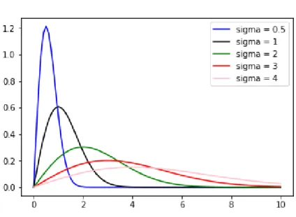
Above equation is valid for all r ≥ 0. The PDF, 2.4 is known as Rayleigh distribution, can be written as 2.12 and is shown in following figure 2.4 with different σ values.: fR(r) = r σ2e −r2 2σ2 (2.12)

This equation too is valid for all r ≥ 0.

2.2.7

Rice Distribution

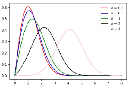
Rician Fading originates from the presence of a direct path. It is described by the Rice distribution, which is:

fR(r) = r σ2e −(r2+A2) 2σ2 I₀(Ar σ2) (2.13)

for all A ≥ 0 and r ≥ 0. Here A is the peak amplitude of the dominant signal and I0(.) is the modified Bessel function of the first kind and zeroth order.

We can define the K factor for this distribution as

KdB = 10 log

A2

2σ2 (2.14)

As A → 0 then KdB → ∞

Figure 2.5: Rice distribution

In conclusion, in the absence of a dominating component the envelope of the received signal is shown to be Rayleigh-distributed (NLOS), while in the presence of a dominant, static component, typically a line-of-sight path, the envelope obeys a Rice distribution. In [12] it is shown how temporal fading is Ricean distributed.

2.3

Signal Representation

In order to take advantage of the theoretical-distribution model, and to un-derstand the statistical properties of the radio channel state, we use the stan-dard in-phase/quadrature (I/Q) representation for band-pass signal analysis.

2.3.1

I/Q Data

I/Q data shows the changes in magnitude (or amplitude) and phase of a sine wave. If amplitude and phase changes occur in an orderly, predeter-mined fashion, since in digital modulations, the information is conveyed by means of appropriate amplitude and phase changes in the transmitted signal [12], I/Q provides a convenient representation for the analysis of these sig-nals [13]. Modulation modifies certain characteristics of a higher frequency carrier signal according to a lower frequency message, or information, sig-nal. I/Q representation is therefore is highly prevalent in Radio Frequency communications systems, and more generally in signal modulation.

Background on Signals

Signal modulation encodes information by changing the parameters of a sine wave. The equation representing a sine wave is as follows:

Accos(2πfct + φ) (2.15)

where Acis the amplitude, fcthe frequency and φ is the phase. The equation

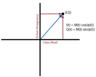
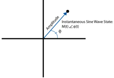
of sine wave above, shows that it is limited to making changes to the ampli-tude, frequency and phase of a sine wave to encode information. Frequency is simply the change rate of the phase of a sine wave (frequency is the first derivative of phase), so frequency and phase of the sine wave equation can be collectively referred to as the phase angle. Therefore, we can represent the instantaneous state of a sine wave with a vector in the complex plane using amplitude (magnitude) and phase coordinates in a polar coordinate system.

We consider now the polar representation of the sine wave in Figure 2.6:

Figure 2.6: Polar representation

It is shown that the distance from the origin to the black point represents the amplitude (magnitude) of the sine wave and the angle from the horizon-tal axis to the line represents the phase. Thus, the distance from the origin to the point remains the same as long as the amplitude of the sine wave is not changing (modulating). The phase of the point changes according to the current state of the sine wave. If the amplitude does not change during one revolution, the dot maps out a circle around the origin with radius equal to the amplitude along which the point travels at a rate of one cycle per second. Because phase is a relative measurement, imagine that the phase reference used is a sine wave of frequency equal to the sine wave represented by the amplitude and phase points. If the reference sine wave frequency and the plotted sine wave frequency are the same, the rate of change of the two sig-nals’ phase is the same, and the rotation of the sine wave around the origin becomes stationary.

In this case, a single amplitude/phase point can represent a sine wave of frequency equal to the reference frequency. Any phase rotation around the origin indicates a frequency difference between the reference sine wave and the sine wave being plotted.

In fact, I/Q data is merely a translation of amplitude and phase data from a polar coordinate system to a Cartesian (X,Y) coordinate system. Using trigonometry, it is possible to convert the polar coordinate sine wave information into Cartesian I/Q sine wave data 2.16 and 2.17.

I(t) = M (t) cos(φ(t)) (2.16)

Q(t) = M (t) sin(φ(t)) (2.17)

IQ data in Communication System

To better understand why IQ data are used in communication systems, it is necessary understand modulation basis. Signal modulation can be divided into two broad categories: analog modulation and digital modulation. Ana-log or digital refers the representation (digital or anaAna-log) of the source data to be modulated. Both analog modulation and digital modulation involve changing the carrier wave amplitude, frequency or phase (or combination of amplitude and phase simultaneously) according to the message data. Am-plitude modulation (AM), frequency modulation (FM) or phase modulation (PM) are all examples of analog modulation. With amplitude modulation, the carrier sine wave amplitude is modulated according to the message signal. The same idea holds true for frequency and phase modulation. For AM, the message signal is the blue sine wave that forms the "envelope" of the higher frequency carrier sine wave. For FM, the message data is the dashed square wave.

As the following figure 2.7 illustrates, this would be the resulting carrier signal changes between two distinct frequency states [12].

Figure 2.7: Time domain representation of AM, FM, and PM Signals [13]

Each frequency state represents the high and low state of the message signal. In the case of the message signal being a sine wave, there would be a more gradual change in frequency, which would be more difficult to see. For PM, notice the distinct phase change at the edges of the dashed square wave message signal.

As mentioned earlier, if only the carrier sine wave amplitude changes with respect to time (proportional to the message signal), as is the case with AM modulation, the I/Q plane graph changes only with respect to the distance from the origin to the I/Q points.

The Figure 2.8 shows that the I/Q data points vary in amplitude only with the phase fixed at 45 degrees. It is not possible to tell much about the message signal, only that it is amplitude modulated. However, the I/Q data points vary in magnitude with respect to time, so, essentially, it is possible see a representation of the message signal.

Figure 2.8: I/Q Data in the complex plane

Why IQ data?

Using a specific tool like LabVIEW’s 3D graph control, the third axis of time to illustrate the message signal can be seen [13]. In result the I/Q data rep-resents the message signal. Because the I/Q data waveforms are Cartesian translations of the polar amplitude and phase waveforms, it may have trouble determining the nature of the message signal. Because amplitude and phase data seem more intuitive, it is better use polar amplitude and phase data instead of Cartesian I and Q data. However, practical hardware design con-cerns make I and Q data the better choice. According to the trigonometric identity [13]:

cos(α + β) = cos(α) cos(β) − sin(α) sin(β) (2.18)

A cos(2πfct + φ) = A cos(2πfct) cos(φ) − A sin(2πfct) sin(φ) (2.19)

= I cos(2πfct) − Q sin(2πfct) (2.20)

Taking 2.20 and the fact that difference between a sine wave and a cosine wave of the same frequency is 90◦ _{phase offset between them into}

considera-tion, the amplitude, frequency and phase of a modulating carrier sine wave can be controlled by simply manipulating the amplitudes of separate I and Q input signals. With this method, it is not necessary to directly vary the phase of an RF carrier sine wave, but it is possible to achieve the same effect by manipulating the amplitudes of I an Q components. Of course, the sec-ond half of the equation is a sine wave and the first half is a cosine wave,so the hardware design must ensure a 90-degree phase shift between the carrier signals used for the I and Q mixers, but this addition is a simpler design issue than the aforementioned direct phase manipulation.

2.4

Cognitive Radio

We must keep in mind that the radio environment where a typical wireless sensor network operates in is becoming more and more complex. This is due to new access to radio technologies and the ongoing densification of network infrastructure in order to meet exponentially increasing capacity demands. Spectrum sharing and coexistence issues both in co-channel and adjacent channel deployments are thus becoming more and more important for ra-dio resource management, in order to avoid excessing interference between wireless networks.

Cognitive wireless networking principles have become an increasingly in-vestigated approach for solving such complex interference management prob-lems in an automated fashion, in particularly without introducing explicit signaling protocols for each combination of interacting wireless technologies. However, using such cognitive approaches requires accurate estimation of the state of the radio environment, in particular forming an understanding of which kinds of wireless technologies are deployed and are causing interfer-ence with the managed network. To improve the quality of wireless commu-nication in IWSNs we introduce signal analysis methods and a classification algorithm to identify radio channel disturbances typical for industrial envi-ronments in the physical layer. Signals analysis methods based on IQ data

and statistical analysis of the magnitude received signal properties help to recognize the temporal disturbances affecting the signal propagation in a radio channel.

2.5

Machine Learning

Machine learning techniques provide powerful tools for signal analysis and classification [14]-[15].

There are many different types of machine learning algorithms, and they are typically grouped by either learning style (i.e. supervised learning, un-supervised learning, semi-un-supervised learning) or by similarity in form or function (i.e. classification, regression, decision tree, clustering, deep learn-ing). After a couple of AI winters and periods of false hope over the past four decades, rapid advances in data storage and computer processing power have dramatically changed the game in recent years. Machine learning was born from pattern recognition and the assumption that computers can learn without being programmed to perform specific tasks.

Machine learning is the science of getting computers to act without being explicitly programmed, but instead letting them learn a few tricks on their own. [17]

The fundamental goal of machine learning algorithms is to generalize be-yond the training samples i.e. successfully interpret data that it has never ‘seen’ before. From a mathematical point of view, machine learning covers problems where we want to learn the "best" mapping f between the input

X and output Y by observing a subset Xtrain ⊂ X. The meaning of "best"

depends on the problem to be solved and if the desired output Y is known or not.

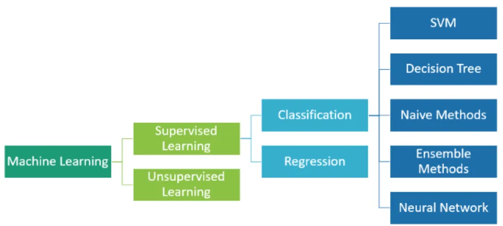
The following image shows a general view of machine learning algorithms, in particular based on classification:

Figure 2.9: General view of machine learning algorithms, with specific interest towards the supervised learning approaches

2.5.1

Unsupervised Learning

Unsupervised machine learning is more closely aligned with what some call true artificial intelligence — the idea that a computer can learn to identify complex processes and patterns without a human to provide guidance along the way. Although unsupervised learning is prohibitively complex for some simpler enterprise use cases, it opens the doors to solving problems that humans normally are not able to tackle. It is used in cases where the input

X is known and the output Y is unknown. The aim of unsupervised learning

is to obtain more information on the input and to learn more about it. For this reason it is difficult to define a correct answer.

2.5.2

Supervised Learning

Supervised learning is the more commonly used learning algorithms. The term supervised learning derives from the requirement that the algorithm’s input (X) and possible outputs (Y ) are already known. For example, a

clas-sification algorithm will learn to identify animals after being trained on a dataset of images that are properly labeled with the species of the animal and some identifying characteristics. In that case, the purpose is to minimize the error between the predicted target ∼y(i) = f (x(i)_{) {x}(i) _{∈ X} and the}

re-al/desired output y(i) _{∈ Y . So, in Supervised learning all the examples must}

be labelled, each case by hand, therefore it may not be a feasible approach for every problem. However, the advantage of labeling the data by hand is that we can decide on the desired outcome of system. It is an convenient approach when historical data is very likely to predict future events.

Regression

The goal of the regression problem is to find an approximating function f from input variables X to a continuous real-valued output variable Y . In these problems, the quantity like amount, price, size is defined such as pre-dicted, therefore the model must be evaluated using an error, like the mean squared error or other metrics. Linear regression is the simplest case of re-gression with the goal to find a linear function that maps inputs and outputs. Focusing on the single-variate case linear regression could be qualified in the following formal way:

wx + b = y (2.21) where w and b are respectively weight and bias and they are the parameter to learn. However, multivariate regression is a more common approach and the model can be derived from the previous one,

K X

k=0

wkxk+ bk= wTx + b = y (2.22)

where w and x are vectors and b is the sum of all biases.

Classification

ap-it and then utilizes this learning in order to classify new observations. This data set may either be simply bi-class (like identifying whether the person is male or female or that the mail is spam or non-spam) or it may be multi-class. Some examples of classification problems are speech recognition or handwriting recognition. In general, classification models can predict the class directly or continuous values that are then converted into probabilities. In the last case, the class with the highest probability is the predicted label. The labels are commonly represented by one-hot encoding, a sparse binary vector with a 1 in the i-th position to indicate the actual class; an example has usually only one class. Since the output is discrete, the classification

ac-curacy can be computed and used as an evaluation measure for the model.

Various classifiers can be found in literature, the most common ones are the following [18]:

• Naive Bayes Classifier (Generative Learning Model): It is a classification technique based on Bayes’ Theorem with an assumption of independence among predictors. In simple terms, a naive Bayes classifier assumes that the presence of a particular feature in a class is unrelated to the presence of any other feature. Even if these features depend on each other or upon the existence of the other features, all of these properties independently contribute to the probability. The naive Bayes model is easy to build and particularly useful for very large data sets. Along with simplicity, naive Bayes is known to outperform even highly sophisticated classification methods.

• SVM: A Support Vector Machine (SVM) is a discriminative classifier formally defined by a separating hyperplane. In other words, given labeled training data (supervised learning), the algorithm outputs an optimal hyperplane which categorizes new examples. The operation of the SVM algorithm is based on finding the hyperplane that gives the largest minimum distance to the training examples. Secondly, this distance receives the important name of margin within SVM’s theory. Therefore, the optimal separating hyperplane maximizes the margin of the training data.

• Decision Trees: The concept of decision trees is that it builds classi-fication or regression models in the form of a tree structure. It breaks down a data set into smaller and smaller subsets while at the same time an associated decision tree is incrementally developed. The final result is a tree with decision nodes and leaf nodes. A decision node has two or more branches and a leaf node represents a classification or decision. The top-most decision node in a tree which corresponds to the best predictor called root node. Decision trees can handle both categorical and numerical data.

• Ensemble Methods: Ensemble methods are meta-algorithms that combine several machine learning techniques into one predictive model in order to decrease variance (bagging), bias (boosting), or improve predictions (stacking).

• Neural Network: A Neural Network (NN) consists of units (neurons), arranged in layers, which convert an input vector into some output. Each unit takes an input, applies a (often nonlinear) function to it and then passes the output on to the next layer. Generally. the networks are defined to be feed-forward: which means that a unit feeds its output to all the units on the next layer, but there is no feedback to the previous layer. Weightings are applied to the signals passing from one unit to another and it is these weightings which are tuned in the training phase to adapt a neural network to the particular problem at hand.

Chapter 3

Related Work

Our focus is on system reliability with specific interest towards classifica-tion of channel disturbances. Different models have been used for interfer-ence/disturbance classification in wireless communication literature. Work such as [14]-[15]-[16] use different techniques to classify disturbance like Sup-port Vector Machine or Random Forrest or Decision Tree classifier that have been already successfully employed for improve wireless communication. All off these, explain how it could possibly include machine learning and wireless communication in different level of art. For example in [15], by combining signal bandwidth, envelope information and their slender extraction, with the intelligently tailored supervised-learning the Authors enable on-board burst-based interference identification, predominantly in real-time. In [14] the focus is instead on the impact of interference from modulated signals and the in-fluence of realistic wireless channel conditions on classification performance. The paper [3] introduces signal analysis and a classification algorithm to iden-tify radio channel disturbance, based on probability density function (PDF) analysis and spectrum analysis. In particular the Authors have arranged an n-dimensional feature vector exploiting shape parameter coming out of Histogram analysis, obtained from I/Q data [13], and RF objects from the spectrum of received signal. Regarding the classification algorithm, they use a practical and simple approach - Nearest Neighbour Rule: samples that

considered environment it is not for typical industrial environments. In [6] the detection of channel state is based on the detection of the shape of the amplitude histogram of received signal, which reveals the nature of inter-ferences in the radio channel. The Authors classify nominal and disturbed channel models as well as disturbance schemes and compare the measured signal against these. The reference channel model classes are acquired by channel simulations.The real environments tests have also been run promis-ing results for disturbances identifications were achieved. The idea is that the most significant has been noticed and that the most significant source of radio signal distortion can be characterized by the shape of the amplitude histograms of the received signal. For example, multipath propagation phe-nomenon result in the broadening of the amplitude of the histogram’s shape, due to the radio waves destructive and constructive interference in which two waves superimpose to form a resultant wave of greater or lower amplitude [6]. In order to compare the histograms of the received signal and predefined channel models’ histograms, we use the chi-squared measure which is typical for expressing similarities/difference of histograms, helping to identify the disturbance.

Our work consists of a mixed approach between [3] and [6]. It means that when considering a typical industrial environments were there will be both large-scale and temporal fading, we introduce a novel histogram approach (of I/Q data) based on PDF analysis and amplitude analysis. Thus, obtaining all features necessary for our classifier. Moreover, we introduce an alterna-tive approach to classify the channel disturbances based on idea [5], that is analyzing the Bit Error Pattern for future improvements of reliability and coexistence of radio systems in these harsh conditions.

Chapter 4

Radio Link Characterization

4.1

Intuition

The idea of our work is based on the concept of introducing some intelligence to each node of the network so that the reliability of the system can be improved. To this end, the intuition could be defined from the following steps:

1. Monitoring: Consists of channel sensing, which means that it has the ability to sense, measure, learn and have an awareness of channel features, the working environment and other requirements. For this purpose, it is useful analyze I/Q data.

2. Problem Detection: During the monitoring phase it is possible to understand that there are problems in the transmission. Thus, it will be necessary to define some metrics that allows us to understand when problems occurs.

3. Problem Identification: When the system detects a problem, the next step is to identify the kind of problem. About that, in our work we define a classification algorithms to understand the signal disturbance. 4. Improvement: Following the identification of the problem, it has been identified that one inelligent step is to apply some countermeasures to

4.2

Classification of the Radio-Link State

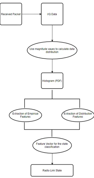
The recognition and identification of the channel properties is based on the signal magnitude analysis with a classifier. The general pattern for classi-fication procedure includes the following phases: pre-processing of measured data, feature extraction from the measured data and classification.

4.2.1

Data Analysis

The data analysis is based on I/Q data of the received packet. In order to take advantage and information from this data representation we need to understand which could be the possible features and properties that reflect an improvement in the classification accuracy.

Amplitude Histogram

A histogram provides a graphical record of the shape of the data distribution. The x-axis shows all the possible values, while y-axis presents the percentage of input samples that each had as a corresponding value. The continuous-valued counterpart of the histogram is the PDF. The histogram is simply an approximation of a PDF; the count of how many samples each possible value has in the range. The strength of the received signal changes with time, due to fluctuations in the gain of the channel caused by multipath fading or electromagnetic interference [6]. The amplitude values of the received signal form a probability density function of a specific form, or in discrete case a specific shape of histogram. By analyzing the features of the histogram shapes of the received signal and comparing them with characteristics being predefined for different radio channels with different characteristics, we can classify histograms into two main categories histograms related to signal; multipath fading (Ricean and Rayleigh distributed) and histograms related to radio interference.

To express the shape of the histogram in a precise way, it useful define four feature values:

1. Mean: It is the mean value of the data.

¯

x =

P

xi

N (4.1)

where xi is the value of data point i and N is the number of data points

2. Spread: It is the average squared deviation of the variable’s values from the mean

spread = P (xi− − x)2 N (4.2)

where xi is the value of data point i and N is the number of data points

and −x is the mean value.

3. Skewness: The skewness reflects the shape or asymmetry of the dis-tribution: if the value is negative, the data spreads out more to the left of the mean, if it is positive, the data spreads out more to the right, and if it is zero, it is symmetric about the mean

skewness = P (xi− − x)3 N (4.3)

4. Peakedness: A single-peaked histogram with a lot of distributional weight in the center and in the tails, but not in the shoulders is said to have “fat tails”; or it is “highly peaked.”

peakedness = P (xi− − x)4 N (4.4)

PDF Analysis of the Received Signal

The PDF analysis is based on the idea that changes in statistical properties of the received signal are strongly correlated with the transitions of the channel states [3].

Thus, matching the PDF of the received signals to the theoretical distri-butions: Ricean 2.5, Rayleigh 2.4, and deriving the PDF´s shape parameters, allows us to numerically characterize the effects of environments disturbances to the channel state.The PDF shape parameters are estimated from sample data by fitting a probabilistic distribution object to the data. To estimate the distribution parameters from the sample data the Maximum likelihood is used. As previously stated, there are two probability models in literature that are commonly used for the propagation channel:

• Rayleigh PDF: fρ(ρ|a, σ) = ρ σ2exp(− ρ2 2σ2) (4.5) • Rician PDF: fρ(ρ|a, σ) = ρ σ2 exp(− ρ2 + a2 2σ2 )Iu( aρ σ2) (4.6)

4.2.2

Classification Model

In our work, the received digitized I(n) and Q(n) samples are pre-processed and analyzed. For each received packet, the PDF of the signal magnitude is estimated as a signal magnitude histogram and match to the theoretical PDF 4.2. In parallel, the amplitude of the histogram is computed and all features are created. How the block diagram 4.1 shows. In particular. from a single received packet: mean, spread, skewness, peakedness can be computed based on the amplitude of the packet. All of these statistical properties, called also

moments in literature, represent the so-called empirical features because

they are obtained from the empirical data, the histogram. On the other hand, the theoretical PDF of the packet is generated, using the empirical/histogram distribution and, from that one, the theoretical distribution is computed by

So, considering 4.6 equation we have that:

• ρ = qI2_{(t) + Q}2_{(t) denotes the magnitude value measured at the}

re-ceiver.

• σ standard deviation of the real part of the time-harmonic multipath component.

• a corresponds to the signal amplitude due to the LOS path in the absence of all other multipath components.

Although, previously, we distinguished between Rician model and Rayleigh model, the Rician model in our case ensures a better fit to the data[12]. From the Rician PDF, the fitting parameter: beta, loc, shape 4.6 are estimated. These are used like features to describe a single packet and in addition from them the goodness of the distribution is computed using the

Kologrov-Smirnov test.

Figure 4.2: Empirical and Theoretical distribution

In statistics, the Kolmogorov–Smirnov test (K–S) is a nonparametric test of the equality of continuous, one-dimensional probability distributions that can be used to compare a sample with a reference probability distribution

(one-sample K–S test), or to compare two samples (two-sample K–S test). The Kolmogorov–Smirnov statistic quantifies a distance between the em-pirical distribution function of the sample and the cumulative distribution function of the reference distribution, or between the empirical distribution functions of two samples [19]. Hence, the value of Kolmogorov-Smirnov test it is also used as a feature. All these properties obtained from the curve fitting could be called like distribution features, because it gives us more information about the general data distribution of the packet.

In conclusion, the feature vector is composed by: • Empirical Features:

Mean Spread Skewness Peakdness Table 4.1: Empirical Features

• Distribution Features:

Beta Location Scale KS-test

Table 4.2: Distribution Features

When all data are collected with the features that allow us to identify the different conditions in the channel and a dataset has been created, the next step is to use it to classify the packet that are affected by disturbances in supervisioned way. The focus of our work is to classify:

• LOS: Line of sight (LoS) is a type of propagation occurring when the transmitter and receiver are in sight, meaning that there is no obstruction of size d such that d » λ, with λ = 1_f the wavelenght of considered signals.

• NLOS: Non-line of sight (NLOS) refers to the path of propagation of a radio frequency (RF) that is obscured (partially or completely) by

Common obstacles between radio transmitters and radio receivers are tall buildings, trees, physical landscape and high-voltage power conduc-tors. While some obstacles absorb and others reflect the radio signal; they all limit the transmission ability of signals.

It could seem as a perfect case where NN would work very well, but gen-erally, neural networks show high variance, high complexity while their set up can be cumbersome. A successful approach to reducing the variance of neural network models is to train multiple models instead of a single one, and to combine the predictions from these models.Furthermore the applica-bility of NN to low-cost WSN hardware is questionable since of the limited computatoinal resources. This is true, specially, if are thinking of using this classification in a online way, where the model has to be loaded every time for each packet. So, it is better to use Ensemble Methods that, according to Ockham’s razor Simplicity leads to greater accuracy, indeed these assume that it uses a combination of models to increase the accuracy, and in addition, they are more soft and easily manageable.

Chapter 5

Experimental Set-up

In this chapter, we talk about the software and the technologies used, then we describe the data collection and preparation.

5.1

LabVIEW

Laboratory Virtual Instrument Engineering Workbench (LabVIEW) is a system-design platform and development environment for visual program-ming language from National Instruments [20].

LabVIEW is commonly used for data acquisition, instrument control and industrial automation on a variety operating systems including Windows, various versions of Unix, Linux and macOS. LabVIEW can create programs that run on those platforms and a variety of embedded platforms, includ-ing Field Programmable Gate Arrays (FPGAs), Digital Signal Processors (DSPs), and microprocessors.

The LabVIEW program development environment is different from stan-dard C or Java development systems in one important aspect: While other programming systems use text-based languages to create lines of code, Lab-VIEW uses a graphical programming language, often called G, to create programs in a pictorial form called a block diagram. Graphical program-ming allows you to concentrate on the flow of data within your application,

A LabVIEW program consists of one or more virtual instruments (VIs). Vir-tual instruments are called as such because of their appearance and operation often imitate actual physical instruments. A VI has three main parts:

• Front panel: It is the interactive user interface of a VI, so named because it simulates the front panel of a physical instrument. The front panel can contain knobs, push buttons, graphs, and many other controls (which are user inputs) and indicators (which are program outputs).

• Block diagram: It is the VI’s source code, constructed in LabVIEW’s graphical programming language, G. The block diagram is the actual executable program. The components of a block diagram are lower-level VIs, built-in functions, constants, and program execution control structures. You draw wires to connect the appropriate objects together to define the flow of data between them. Front panel objects have corresponding terminals on the block diagram so data can pass from the user to the program and back to the user.

• Icon: In order to use a VI as a subroutine in the block diagram of another VI, it must have an icon. A VI that is used within another VI is called a subVI and is analogous to a subroutine. The icon is a VI’s pictorial representation and is used as an object in the block diagram of another VI.

5.1.1

USRP

Universal Software Radio Peripheral (USRP) is a range of Software-Defined Radios (SDR) designed and sold by Ettus Research and its parent company, National Instruments used for RF applications [20]. USRP transceivers can transmit and receive RF signals in several bands, and you can use them for applications in communications education and research. It supports Linux, MacOS, and Windows platforms. Several frameworks including GNU Radio, LabVIEW, MATLAB and Simulink use UHD. The functionality provided by UHD can also be accessed directly with the UHD API, which provides native