Scuola di Scienze
Dipartimento di Fisica e Astronomia Corso di Laurea Magistrale in Fisica
ClinQC: quality control of an X-ray
imaging system using clinical images
Relatore:
Prof.ssa Maria Pia Morigi
Correlatori:
Dott. Wouter J. H. Veldkamp
Dott.ssa Pieternel van der Tol
Dott. J. Chiel den Harder
Prof. Berend C. Stoel
Presentata da:
Lisa Bravaglieri
The work presented in this thesis is part of a research project of Leiden University Medical Center (LUMC) in The Netherlands. It belongs to the field of Diagnostic Radiology analysed from a Medical Physics point of view. After a short overview of the weekly quality controls of an X-ray imaging device, performed using simple phan-toms, the thesis focuses on a novel approach called ClinQC (Clinical images-based Quality Control): it has the purpose to monitor the stability of imaging devices, aiming at the early detection of changes in image quality or radiation dose, by de-riving quality parameters from chest images of routine patient examinations. The ClinQC algorithm extracts the noise from clinical images and derives the main dose quantities. The noise study presented in this thesis comprehends a validation of the algorithm, performed in several ways: image deteriorations, simulations, phantom studies and real clinical examples. For dose and homogeneity studies only some pre-liminary results are presented. The thesis collects also some ideas of improvement that can be considered for the future versions of the algorithm and to extend the ClinQC project to other X-ray anatomies and imaging modalities.
The obtained similar results for the two compared methods prove that ClinQC is able to give immediate feedbacks of the quality of the imaging devices using patient images. It provides reliable, on-the-fly and sensitive parameters of the quality of the X-ray imaging system, that have the same physical meaning and similar relative variation as the quality indicators of the gold standard QClight method. It can be concluded that the ClinQC algorithm could be already applied in clinical practice, with the initial support of the QClight weekly quality control. In this way, a com-parison between the two methods in a real test period will be a guide to find the necessary adjustments of the algorithm until the final version is being installed and stably used in clinical practice.
Il lavoro presentato in questa tesi ´e parte di un progetto di ricerca dell’ospedale universitario Leiden University Medical Center (LUMC) dei Paesi Bassi. La tesi si inserisce nel campo della Radiologia Diagnostica dal punto di vista della Fisica Medica. Dopo una breve panoramica sui controlli settimanali di qualit´a di un sis-tema di diagnostica per immagini a raggi X, eseguiti con semplici fantocci, la tesi si concentra su un nuovo approccio chiamato ClinQC (Clinical images-based Quality Control). Esso ha lo scopo di monitorare la stabilit´a del dispositivo, mirando alla rilevazione precoce delle variazioni nella qualit´a delle immagini o nella dose di ra-diazioni, derivando parametri di qualit´a a partire da immagini di esami di routine al torace dei pazienti. L’algoritmo ClinQC estrae il rumore dalle immagini cliniche e ricava le principali grandezze dosimetriche. Lo studio sul rumore presentato in questa tesi comprende la validazione dell’algoritmo, eseguita in diversi modi: dete-rioramento delle immagini, simulazioni, studi su fantocci ed esempi clinici reali. Per quanto riguarda gli studi di dose ed omogeneit´a, sono illustrati solo alcuni risultati preliminari. La tesi raccoglie anche alcune idee di miglioramento per le future ver-sioni dell’algoritmo e per estendere il progetto ClinQC ad altre anatomie e modalit´a di imaging.
I risultati simili ottenuti per i due metodi a confronto dimostrano che ClinQC ´e in grado di dare un’immediata valutazione della qualit´a del dispositivo utilizzando le immagini dei pazienti e, in particolare, fornisce affidabili e sensibili parametri di qualit´a dei sistemi di diagnostica per immagini a raggi X, che hanno lo stesso significato fisico e simili fluttuazioni relative degli indicatori di qualit´a utilizzati nel metodo standard di riferimento QClight. Si pu´o concludere che l’algoritmo ClinQC potrebbe gi´a essere applicato nella pratica clinica, con il supporto iniziale del con-trollo di qualit´a settimanale QClight. Un vero periodo di prova e confronto tra i due metodi, servir´a anche come guida per effettuare gli aggiustamenti necessari all’algoritmo finch´e la versione finale non venga installata e stabilmente utilizzata nella pratica clinica.
1 Introduction 3
2 Background 5
2.1 A typical chest X-ray imaging system . . . 5
2.2 QClight: phantom-based quality control . . . 9
2.3 ClinQC: clinical images-based quality control . . . 12
3 Noise study 15 3.1 Methods . . . 15
3.1.1 ClinQC algorithm: noise extraction from clinical images . . . 15
3.1.1.1 Properties of the ClinQC extracted noise images . . . 19
3.1.2 The ClinQC algorithm - alternative versions . . . 20
3.1.2.1 Grid sampling approach . . . 20
3.1.2.2 ClinQC applied to mammography . . . 21
3.1.3 Validation of the ClinQC algorithm . . . 23
3.1.3.1 Image deterioration study . . . 23
3.1.3.1.1 Blur . . . 23
3.1.3.1.2 Gaussian noise . . . 24
3.1.3.2 Statistical analysis with simulations . . . 27
3.1.3.2.1 Step simulation . . . 27
3.1.3.2.2 Trend simulation . . . 29
3.1.3.3 The ClinQC performance in clinical practice . . . 31
3.1.3.4 Outlier analysis . . . 31
3.1.3.5 Image Pyramids noise extraction algorithm comparison . . 33
3.1.3.6 Phantom comparisons . . . 34
3.2 Results . . . 37
3.2.1.3 The ClinQC noise values: Relevant clinical examples . . . . 45
3.2.2 The ClinQC algorithm - alternative versions: validation . . . 47
3.2.2.1 Grid sampling approach . . . 47
3.2.2.2 ClinQC applied to mammography . . . 50
3.2.3 Image deterioration study . . . 53
3.2.3.1 Blur . . . 53
3.2.3.2 Gaussian noise . . . 58
3.2.4 Statistical analysis with simulations . . . 63
3.2.4.1 Step simulation . . . 63
3.2.4.2 Trend simulation . . . 67
3.2.5 The ClinQC performance in clinical practice . . . 69
3.2.5.1 Detection of flipped anti-scatter grid . . . 69
3.2.5.2 Detection of anti-scatter grid replacement . . . 74
3.2.6 Outlier analysis . . . 75
3.2.7 Image Pyramids noise extraction algorithm comparison . . . 78
3.2.8 Phantom comparisons . . . 82
3.3 Discussions . . . 86
3.3.1 The ClinQC algorithm: noise extraction from clinical images . . . . 86
3.3.1.1 Properties of the ClinQC extracted noise images . . . 86
3.3.1.2 The ClinQC noise values: baseline . . . 88
3.3.1.3 The ClinQC noise values: Relevant clinical examples . . . . 88
3.3.2 The ClinQC algorithm - alternative versions . . . 89
3.3.2.1 Grid sampling approach . . . 89
3.3.2.2 ClinQC applied to mammography . . . 89
3.3.3 Image deterioration study . . . 90
3.3.4 Statistical analysis with simulations . . . 91
3.3.4.1 Step simulation . . . 91
3.3.4.2 Trend simulation . . . 91
3.3.5 The ClinQC performance in clinical practice . . . 92
3.3.6 Outlier analysis . . . 93
3.3.7 Image Pyramids noise extraction algorithm comparison . . . 94
4.1 Methods . . . 95
4.1.1 Exposure and tube output . . . 95
4.2 Results . . . 97 4.2.1 Exposure . . . 97 4.2.2 Tube output . . . 98 4.3 Discussion . . . 100 5 Homogeneity study 103 5.1 Methods . . . 103 5.1.1 Thresholding algorithms . . . 103 5.1.2 Normalized profiles . . . 104 5.1.3 Validation method . . . 105 5.2 Results . . . 106 5.3 Discussion . . . 111
6 Discussions and conclusions 113
1.1 The main building entrance of LUMC. . . 3
2.1 A chest X-ray imaging system at LUMC. . . 6
2.2 The three ionization chambers of the AEC on an LUMC bucky system. . . 7
2.3 The QClight phantom is positioned for image acquisition. . . 9
3.1 Original image. . . 16
3.2 Smoothed image. . . 16
3.3 High spatial frequencies image. . . 17
3.4 Normalized high spatial frequencies image. . . 17
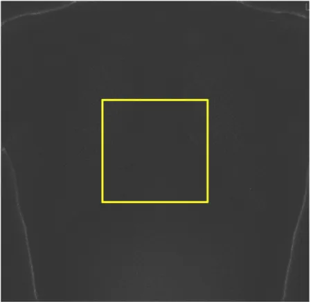
3.5 The ROI selected for the noise measurement on the ClinQC normalized noise image. . . 18
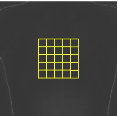
3.6 An example of the sampling grid that can be used to improve the ClinQC noise extraction algorithm. . . 21
3.7 Graphic reproduction of how a step in the noise values would appear. . . . 27
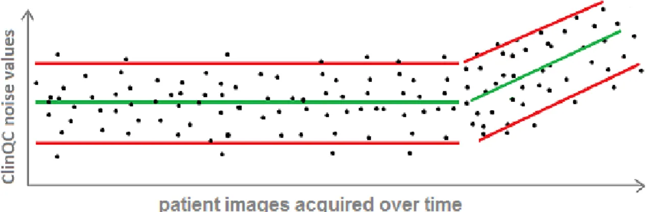
3.8 Graphic reproduction of how a trend in the noise values would appear. . . . 29
3.9 Example of Gaussian and Laplacian Pyramids. . . 34
3.10 RANDO anthropomorphic phantom. . . 35
3.11 An example of high-low frequencies plot of the ClinQC high frequencies map, the output of the algorithm at the first step, before the normalization. 37 3.12 An example of high-low frequencies plot of the ClinQC normalized noise map, the final output of the algorithm after the second step of the normal-ization. . . 38
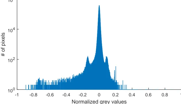
3.13 The histogram of the ClinQC normalized noise map. This corresponds to the high-low frequencies plot shown in Fig. 3.12. . . 39
3.14 The result of the histogram-based segmentation performed on the ClinQC normalized noise image. . . 40
3.16 Histogram of the central ROI (yellow) cropped from the ClinQC normalized noise map (light blue). . . 42 3.17 The ClinQC noise values baseline. . . 43 3.18 Distribution of the ClinQC noise values baseline, where the black dashed
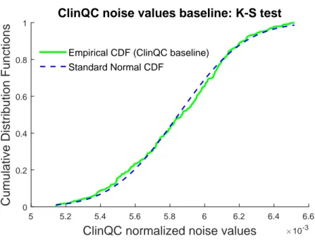
line is the normal fit of the histogram. . . 44 3.19 Estimated CDF of the ClinQC noise values baseline dataset, and standard
normal CDF compared by the K-S test. . . 44 3.20 The ClinQC noise values historical examples. . . 45 3.21 Distribution of the ClinQC noise values obtained using the grid sampling
approach for Patient # 1. In red: mean value of the distribution. In green: median value of the distribution. . . 47 3.22 Distribution of the ClinQC noise values obtained using the grid sampling
approach for Patient # 2. In red: mean value of the distribution. In green: median value of the distribution. . . 48 3.23 Comparison of the ClinQC original algorithm and the ClinQC modified
method using the sampling grid approach for the images of the baseline (Section 3.2.1.2). . . 48 3.24 Patient with pacemaker. . . 49 3.25 Patient with medical device. . . 49 3.26 Histogram of the biggest differences in percentage in the ClinQC noise
val-ues obtained using the ClinQC original algorithm and the ClinQC modified algorithm using the sampling grid approach, for the images in the baseline period (Section 3.2.1.2). . . 50 3.27 A typical mammogram. . . 51 3.28 The ClinQC noise map of a mammogram with the ROI marked in yellow. . 51 3.29 The ClinQC noise values, exposure and kVp computed on the dataset of
mammograms and tomosynthesis reconstructed projections. . . 52 3.30 Output of the image deterioration study that shows the decrease of the
mean of the noise values measured after blurring, with different increasing amounts of blur, 41 different groups of 50 images, together with the first blue group made of 50 original X-ray images of the chest. . . 53 3.31 The decrease in percentage of the mean of the noise values measured during
3.33 A detail in the lung of a patient chest X-ray image after blurring with σ = 1 pixel. . . 55 3.34 Output of the image deterioration study that shows the decrease of the
spread of the noise values measured after blurring, with different increasing amounts of blur, the same group of 25 original X-ray images of the chest. . 56 3.35 The increase in percentage of the relative spread of each group of noise
values of the deteriorated images measured during the image deterioration study with blurring. . . 57 3.36 Output of the image deterioration study that shows the increase of the
mean of the noise values, measured after the addition of Gaussian noise with 0 mean and variances computed in order to achieve prefixed levels of deterioration of the estimated SNR of different random sub-sampled groups of 25 original chest X-ray images. . . 58 3.37 The increase in percentage of the mean of the noise values measured during
the image deterioration study with Gaussian noise. . . 59 3.38 A detail in the lung of a patient chest X-ray image. . . 60 3.39 A detail in the lung of a patient chest X-ray image after addition of Gaussian
noise, with 0 mean and variance computed in order to achieve a decrease of the estimated SNR by 30%. . . 60 3.40 Output of the image deterioration study that shows the increase of the
spread of the noise values, measured after the addition of Gaussian noise with 0 mean and variances computed in order to achieve prefixed levels of deterioration of the estimated SNR of different random sub-sampled groups of 28 original chest X-ray images. . . 61 3.41 The increase in percentage of the relative spread of the noise values
mea-sured during the image deterioration study with Gaussian noise. . . 62 3.42 Rejection ratio (%) resulting from the step simulation when the baseline
was increased by 3%. . . 63 3.43 Final output curve of the step simulation (pink). The light blue stars
repre-sent the output values of the two simulations of the anti-scatter grid removal and replacement. . . 64 3.44 Rejection ratio (%) obtained with the step simulation of the anti-scatter
3.46 Example of the one month time line of the simulated ClinQC noise values generated by the trend simulation. . . 67 3.47 Example of the rejection ratio (%) obtained performing the trend simulation
on the month time line. . . 68 3.48 Output curves of the trend simulations performed on the one week time line
and the one month time line. . . 69 3.49 The appearance of a typical QClight phantom image acquired during the
weekly QC. . . 70 3.50 The appearance of QClight phantom image acquired with a flipped
anti-scatter grid. . . 70 3.51 The appearance of one patient image acquired in 2015 with the same
imag-ing system now in use. . . 71 3.52 The appearance of the same patient image acquired in 2016 with the
anti-scatter grid flipped. . . 71 3.53 The noise values and the exposures measured on all the clinical images of
the week when the anti-scatter grid was flipped in July 2016. . . 72 3.54 The result of the alerts produced by a moving window of size 12 images
moved along the ClinQC noise values of all the images of the complete week when the anti-scatter grid was flipped in July 2016. . . 73 3.55 Representation of ClinQC noise values and exposures recorded from
regu-lar clinical data (in blue) and clinical data from images acquired with the flipped anti-scatter grid (in red), with lateral distributions. . . 74 3.56 The result of the alerts produced by a moving window of size 19 images
moved along the ClinQC noise values of a dataset of clinical chest X-ray images at the turn of the anti-scatter grid update occurred at the end of 2014. . . 75 3.57 The ClinQC noise values of all the clinical images acquired with the
ac-tual system setup displayed in a time line; in red are marked the outliers according to the baseline red acceptance limits. . . 76 3.58 The exposures of all the clinical images acquired with the actual system
setup displayed in a time line; in red are marked the exposures of the outlier images in terms of the noise (Fig. 3.57). . . 77
male patients. . . 77
3.60 L1 Pyramid image example. . . 78
3.61 L1 norm Pyramid image example. . . 78
3.62 High-low frequencies plot of L1 Pyramid image. . . 79
3.63 High-low frequencies plot of L1 norm Pyramid image. . . 79
3.64 Histogram of L1 Pyramid image. . . 79
3.65 Histogram of L1 norm Pyramid image. . . 79
3.66 The comparison between the ClinQC normalized noise values and the Pyra-mid normalized and not normalized noise values measured on all the images forming the baseline dataset. . . 80
3.67 The correlation between the ClinQC algorithm and the Pyramid (normal-ized) algorithm. . . 81
3.68 The blurring-induced decreasing effect (in blue) and the exposure-induced increase (in red) of the ClinQC noise values, measured on RANDO images, and the QClight noise values. . . 82
3.69 The 2D NPS of the QClight images acquired at different exposure levels. . . 83
3.70 The 2D NPS of the QClight images blurred with different σ of Gaussian blurring kernels. . . 83
3.71 The 2D NPS of RANDO images acquired at different exposure levels. . . . 83
3.72 The 2D NPS of RANDO images blurred with different σ of Gaussian blur-ring kernels. . . 84
3.73 A comparison between the ClinQC and the QClight methods applied on the history dataset of, respectively, one clinical chest X-ray image per week and one phantom image per week. . . 84
4.1 Exposure (mAs) of the ClinQC baseline dataset with lateral distribution, with red acceptance limits of±2σ. . . 97
4.2 Tube output (mGy/mAs) of the ClinQC baseline dataset and DAP (mGycm2) of the QClight history data of 2015/2016. . . 99
4.3 Output curve of the step simulation applied to clinical tube output values. . 100
5.1 Example of how the normalized profiles algorithm divides one chest patient image in two vertical sides and draws a vertical profile of the pixels on the left rows (yellow) and one on the right rows (pink). . . 105
highlighted black class represents mainly the background and ends at the 350th grey level. . . 107 5.4 Example of the segmentation of the background pixel values in a chest X-ray
image using the Fast Marching Method (FMM). . . 108 5.5 Left side: each box represents the distributions of the inhomogeneity
val-ues obtained applying the specified clinical homogeneity algorithm on the baseline dataset. Right side: comparison between the normalized profiles algorithm and the QClight method, both applied on the history dataset. The y-scale is zoomed. . . 108 5.6 Top: the inhomogeneity values computed using the normalized profiles
al-gorithm on the history dataset of clinical images. Bottom: the inhomo-geneity values computed using the QClight method on the history dataset of QClight phantom images. . . 109 5.7 Example of a strong simulated anode heel effect on a clinical chest X-ray
image. . . 110 5.8 Example of the segmentation using the FMM on the same chest X-ray
image, respectively in its original appearance (left) and after simulating two different strength of the anode heel effect with gradients of 1 (center) and 5 (right) grey values for 100 pixel. . . 111 5.9 Example of the primary X-ray beam shadow, that appears as an image
AEC Automatic Exposure Control CDF Cumulative Distribution Function
ClinQC Clinical images-based Quality Control CoV Coefficient of Variation
CT Computed Tomography DAP Dose Area Product
DICOM Digital Imaging and Communications in Medicine ECMP European Congress of Medical Physics
FMM Fast Marching Method FOV Field Of View
JOP Young Researcher Prize K-S Kolmogorov-Smirnov kVp peak kilovoltage
LAT Lateral chest X-ray projection LUMC Leiden University Medical Center LUT Look-Up Table
NPS Noise Power Spectrum
NVKF Dutch Society for Medical Physics PA Postero-Anterior chest X-ray projection PACS Picture Archiving Communication System QC quality control
QClight light (phantom-based) Quality Control REX Reached Exposure
ROC Receiver Operating Characteristic ROI Region Of Interest
SDD Source-DAP-meter Distance SID Source-Image Distance SNR Signal to Noise Ratio
Introduction
This Master’s thesis is the result of my six months internship within the group of Medical Physics at the Radiology Department of Leiden University Medical Center (LUMC) in The Netherlands [1]. LUMC is a modern university medical center for research, education and patient care with a high quality profile and a strong scientific orientation, that employs around 7000 people (Fig. 1.1). I had the chance
Figure 1.1: The main building entrance of LUMC.
to work at LUMC from March until August 2016 as one of the students that won the Erasmus+ : Mobility for Traineeship competition [2] with the ClinQC project
(Clinical images-based Quality Control).
This project started at LUMC in 2015 after some initial ideas by the two medical physicists in training J. Chiel den Harder and Pieternel van der Tol, resulting in an algorithm that was further developed under the lead of the medical physicist Wouter J. H. Veldkamp, in the group of Medical Physics of LUMC headed by Koos Geleijns. Their aim was to perform a quality control (QC) of an X-ray imaging system without the use of routine phantoms, instead performing measurements of dose and image quality on the large number of clinical images of patient studies acquired with the system everyday. The use of clinical image quality with the purpose to early detect any quality regression of diagnostic X-ray machines is an innovative approach. I entered the project under the lead of the previously mentioned medical physicists and of Berend C. Stoel (associate professor at the Division of Image Processing, Radiology Department, LUMC), because there was the need of a student to do additional analysis to show the benefit of implementing this QC algorithm in the daily clinical practice of the imaging systems at Radiology Department. In fact, the goal of my internship and the aim of this Thesis was to validate the existing algorithm for the QCs of the diagnostic X-ray imaging device and to invent or develop new measures of the quality of the system based on the planar chest radiograph of the patients. More details about the starting point of the ClinQC project and my role in it are explained at the end of Chapter 2.
The Thesis is structured in three main subjects: Dose study (Chapter 4), Noise study (Chapter 3) and Homogeneity study (Chapter 5). Each Chapter is divided in three main Sections: Methods, Results and Discussion. The final Chapter, Discussion and Conclusions (Chapter 6), will give an overview of the ClinQC project achievement and an outlook for future steps. The focus will mostly be on the Noise study (Chapter 3), the ClinQC algorithm validation and its improvements, since I mainly worked on this topic during my internship. The Homogeneity Chapter (Chapter 5) contains a pilot study that still needs some improvements and a concrete validation before it can be applied in clinical practice.
Before going through these main topics, the specific properties of the analysed chest X-ray imaging system will be discussed in Section 2.1 and the currently existing procedure to measure its quality and stability using phantom images in Section 2.2.
Background
2.1
A typical chest X-ray imaging system
The chest X-ray is one of the most commonly performed diagnostic X-ray exami-nations; it evaluates the lungs, heart and chest wall. The basic equipment typically used for chest X-rays consists of an X-ray tube producing a divergent beam and a wall-mounted bucky system (Fig. 2.1), containing the digital flat panel detector, the anti-scatter grid and the ionization chambers of the AEC [3]. In this kind of ex-amination the X-ray tube is positioned at 2.00 m Source-Image Distance (SID) from the detector, this can vary for other examined anatomies. Two views of the chest are taken, one from the back where the patient stands with hands on hips and chest pressed against the image plate, Postero-Anterior chest X-ray projection (PA), and the other from the side of the body, Lateral chest X-ray projection (LAT), where the patient stands against the image recording plate holding the bucky. In this thesis only chest PA projections will be analysed.
In the next paragraphs some of the components of the imaging system matter of interest for this thesis will be illustrated, along with the patient acquisition protocol and the output image format and processing.
Figure 2.1: A chest X-ray imaging system at LUMC.
Components
Anti-scatter grid The anti-scatter grid is the mobile device that is placed be-tween the patient and the detector and that reduces the arrival of scattered radiation to the detector, decreasing the noise and enhancing the contrast in the X-ray im-age. The grid is designed with a series of alternating strips of lead and air that are angled to match the divergence of the X-ray beam. The primary beam radiation passes through the space between the lead strips only if it travels parallel to them, but scattered radiation which deviates from the divergent beam encounters the lead strips at a different angle, defined by the grid focal distance, and is attenuated from the beam. This device is useful in examinations where a large quantity of scattered radiation is created, with large tissue thicknesses and high peak kilovoltage (kVp). The employment of a grid requires a greater exposure to the patient since the pri-mary beam is also attenuated by the lead strips [4].
AEC The Automatic Exposure Control (AEC) has the purpose to deliver con-sistent, reproducible exposures across a wide range of anatomical thicknesses and kVp [4]. On the detector there are three ionization chambers that count the number of photons that pass through the patient in three positions of interest: the spine in the center, and the two lung regions left and right (Fig. 2.2). The manufacturer
Figure 2.2: The three ionization chambers of the AEC on an LUMC bucky system.
does not share its complete knowledge about the functioning of this device, but what is known is that the results of the three chambers are combined in a unique output that allows to stop the X-ray exposure when the detector receives the desired dose in at least one of those three areas. For example, if a patient has an implant like a pacemaker, the sensor behind it will receive less photons than the other two and the AEC, according only to that output, would increase the exposure time, but the contribution of the other two ionization chambers will stop the source after a shorter exposure time.
Anode heel effect The anode heel effect appears in X-ray images as a gradient in the pixel values, due to the reduction of the intensity of the X-ray beam towards the anode side of the inner geometry of the tube [4]. This effect could change in appearance when the anode deteriorates over time, and this might produce in the images a more evident gradient in the grey values. This is an information about the
quality of the imaging system that can be retrieved from phantom images performing a QC (Section 2.2).
Acquisition protocol
The acquisition protocol is set up in order to obtain the optimal image quality for a diagnosis with the lowest patient dose. For an average weighted adult patient the typical acquisition protocol for a PA chest X-ray examination is:
SID = 2.00 m kVp = 133 kV
(gives the optimal contrast between the different body tissues and organs) AEC = ON
(automatically corrects for different body thicknesses) image post-processing = ON
DICOM images and digital processing
The Digital Imaging and Communications in Medicine (DICOM) is the standard for handling, storing, printing, and transmitting information in medical imaging. The DICOM images are characterised by a header of DICOM tags that contain all the available technical data regarding the imaging system and the acquisition together with patient information [5].
The X-ray raw image that is captured by the detector sensors is always processed. This first image processing is the collection of operations and filtering that are applied on the digital images just after their acquisition, it is usually called pre-processing and compensates for different gain of different detector areas. This is an automated algorithm implemented by the manufacturer and is not accessible by the user: it can be said that the pre-processing is a black-box to the user.
Other operations and filtering, such as noise reduction in the background, are cho-sen by the user when selecting a chest X-ray protocol and can be classified as post-processing. Then there is additional post-processing, that can be adapted by the user by applying the appropriate parameter settings in the acquisition protocol and
that controls the Look-Up Table (LUT) and filtering like edge-enhancement. For patient examinations this post-processing is always used, but for some analysis with phantoms it can be useful to set it OFF switching the acquisition protocol. The post-processing is defined based on the clinicians experience with the aim to im-prove the diagnostic quality of the image.
2.2
QClight: phantom-based quality control
The quality control of a diagnostic X-ray imaging system comprises monitoring and evaluation of all characteristics of performance that can be measured and con-trolled [6]. The QC should not only measure the technical stability of the system, but also the dose given to the patients and the resulting image quality, that are relevant parameters for radiation protection and for a correct diagnosis made by the radiologist. Nowadays the most common way to measure these features is the employment of phantoms that are particularly designed to produce the same global attenuation of the X-ray beam intensity as a patient body [7].
QClight is the name of the approach and the phantom that are currently used at LUMC for weekly QCs in planar X-ray systems. QClight is a 2 mm thick copper plate phantom that has to be placed in front of the beam exit passage from the tube (Fig. 2.3). Each monday morning, before the first patient, the radiographer
places the QClight uniform phantom in this position and acquires with a specific protocol three images, activating the three ionization chambers of the AEC one at a time: only with three images it is possible to see if the three devices are working in the same consistent way to produce the desired combined AEC result (Section 2.1). The acquisition protocol of QClight phantom images is defined by some rules. The most important for our aim are:
SID = 1.50 m
(this distance is standardized for all the QClight acquisition protocols of LUMC: it is the same for all the X-ray rooms where different body anatomies are imaged)
kVp = 133 kV
(this is the same kVp used for adult patients who come for a chest X-ray examination)
AEC = ON (in only one ionization chamber at a time) image post-processing = OFF
From the acquired images it is possible to retrieve all the necessary information that allow to assess a QC of the X-ray imaging system, including some dose parameters and image quality figures that are directly related to the system performances.
Dose The main dose quantities [8] are available in the DICOM tags of the QClight images: exposure, peak kilovoltage (kVp), Reached Exposure (REX) and Dose Area Product (DAP) for example. It is also possible to derive some other dose parame-ters to gain more complex information, combining different existing quantities given from the manufacturer of the X-ray imaging system (Chapter 4).
The constancy of all these dose parameters within their conventionally accepted ranges is investigated each monday with the QClight analysis; then, if the QC regis-ters some differences from the usual behaviour of the system, an alarm is produced and the medical physicist job is to find out what are the causes and a possible so-lution.
Noise The noise in an image is the stochastic variation in the signal that compro-mises the image quality. The presence of the noise in X-ray images is due to three major causes. First, there is a statistical component, namely quantum noise, inher-ent to the fluctuations of the electromagnetic field that make the noise in the image depend on the intensity of the X-ray source: if the exposure (mAs) is increased the noise becomes higher, but the signal increases faster with increasing mAs, so the noise-to-signal ratio decreases, and in medical imaging this translates in giving higher dose to the patients. Second, all the electronic components of the system, mainly the digital detector, generate noise and interferences in their outputs that appear in the image as electronic noise. Then, the noise is due for large part to the scattered radiation that results from the interaction between the X-ray primary beam and patient tissue. A QC that includes the monitoring of some image quality figures, like the noise, gives the chance to check both the detector performances, together with all the electronic parts of the system, and the patients exposure [9]. The QClight images are homogeneous, so their pixel grey values fluctuations directly represent the noise. Selecting a Region Of Interest (ROI) of 30 % of the Field Of View (FOV) in the center, for example, makes it possible to quantify the amount of noise as the standard deviation of the pixel values that belong to this ROI. Since the system deals with an AEC that may change the exposure time for each QClight image that is acquired every week, the average grey value of the QClight image could be varying among all the acquisitions, giving to the noise measure a dependence to the image intensity that can easily be corrected. So the normalized QClight noise indicator is defined as
N oise QClight = σµROI
ROI = s 1 N M −1 N P i=1 M P j=1 (p(i, j)− µ)2 µ , (2.1)
where N M is the number of pixels p(i, j) inside the selected ROI of the image, σ is the standard deviation of their grey values and µ is the average
µROI = 1 N M N X i=1 M X j=1 p(i, j). (2.2)
Homogeneity Another image quality figure that is linked to the system perfor-mances is the image homogeneity. It reflects in particular the uniformity of the response of the detector. The QClight image is expected to be homogeneous as the phantom attenuation is, except for the inhomogeneities due to the detector mal-functioning or non-uniform response and inhomogeneities in the X-ray beam. There are many formulas to measure this quantity on an image of a uniform phantom, the
one used at LUMC takes into account five square ROIs (R1, R2, ... , R5) of width
approximately 20 % of the FOV, one in the center of the image and the others close to the four corners. The average pixel value µ in each one of these five ROIs is computed using Eq. 2.2. Then the inhomogeneity is defined as:
Inhomogeneity (%) = max(µR1, µR2, ..., µR5)− min (µR1, µR2, ..., µR5) mean (µR1, µR2, ..., µR5)
%. (2.3)
2.3
ClinQC: clinical images-based quality control
The long term goal of the ClinQC project will be the replacement of phantom-based QCs with measurements based directly on clinical images that will give a complete overview of the efficiency of the X-ray imaging devices. With the current imaging system for the chest, there is a need of a weekly standardized procedure to monitor its constancy using phantoms, i.e. the QClight analysis, but with other X-ray imag-ing modalities the QClight is not performed. This method required the trainimag-ing of the radiographers for the phantom acquisition procedure and 10 minutes per week to be performed. That is why it seems simpler and quicker to use a clinical images-based approach measuring the stability of the X-ray imaging device images-based on clinical images. The ClinQC method enables more frequent QCs, even for X-ray anatomies and imaging modalities where the QC measurements are not available. In addition, with this innovative approach, it is also possible to enter the universe of big data, us-ing the large statistics of hospitals made by thousands of patient images: at LUMC approximately 50 patients/day come for a chest X-ray examination, which makes a total amount of 250 patients/week, 1000 patients/month and 12 000 patients/year. In 2015 at LUMC a new clinical images-based QC was developed: the ClinQC algo-rithm now monitors different dose parameters and the noise of the imaging system from patient images, while the homogeneity measure is still in progress. With these
measurements on each new clinical image, the ClinQC algorithm now provides a significant knowledge about the stability of the system, and it can work side by side with the QClight method to validate the ClinQC tool.
The aim of this Thesis is to show all the steps of the ClinQC algorithm validation process that I implemented during my internship at LUMC and an important exam-ple of how the Noise and Exposure measurements would work if applied in clinical practice.
After the first steps of the ClinQC project, it has been presented in two important occasions. In 2016 J. Chiel den Harder gave a talk about the ClinQC project and received the Young Researcher Prize (JOP) for the best scientific presentation of the Dutch Society for Medical Physics (NVKF). In the same year Pieternel van
der Tol presented the ClinQC project at the 1st European Congress of Medical
Physics (ECMP) in Athens, Greece [10]. Moreover the work shown in this Thesis will hopefully be published as a scientific paper in 2017.
Noise study
3.1
Methods
In this Section all the methods adopted and developed to implement and validate the ClinQC noise extraction algorithm are illustrated.
3.1.1
ClinQC algorithm: noise extraction from clinical
im-ages
In 2015 at LUMC the ClinQC algorithm was invented [11], which extracts the noise
directly from chest patient images in two main steps1.
1. Subtraction from the chest original image (Fig. 3.1) of a smoothed version of the same image (Fig. 3.2). The smoothing is obtained with a Gaussian
blur-ring filter with a kernel of 7×7 pixel size (pixelsize = 0.12×0.12 mm), shaped
as a Gaussian distribution defined with σ = 0.6 pixel. The smoothed image is a version of the original image where the noise is partially removed: so it contains mainly the low spatial frequencies, which represent the anatomical signal. The output of this subtraction is the ClinQC high spatial frequencies
map (Fig. 3.3): this image contains mainly noise but also some body signal,
in the example the lung region can clearly be distinguished from the abdomen
region. To measure the noise directly on this first image would result in a sig-nificant patient dependent noise parameter, and the aim of the ClinQC project is to find patient-independent measurements of the quality and stability of the system that are not affected by patient variability.
2. Normalization of the ClinQC high spatial frequencies map by the smoothed
low frequencies image is then required for two different reasons. First, to
remove the dependence to the different image intensities that vary among all the patients examinations due to the presence of the AEC device: for the same purpose, in the QClight noise measure (Section 2.2) the normalization is represented in Eq. 2.1 by the ratio of each image to its average pixel value µ. Second, the image normalization is implemented also to try to remove the evident remaining body signal from the noise map. From the example in Fig. 3.4 it is clear that the new obtained ClinQC normalized noise map contains less patient anatomical signal than the output image after step 1 (Fig. 3.3), in fact only the main patient external edges can be seen.
Figure 3.1: Original image. Figure 3.2: Smoothed image.
The final step to extract the noise from clinical images using the ClinQC algorithm consists in drawing a big ROI (Fig. 3.5) in the middle of the ClinQC normalized
Figure 3.3: High spatial frequencies im-age.
Figure 3.4: Normalized high spatial fre-quencies image.
way, the ClinQC normalized noise value can be computed as the standard deviation of the pixels p(i, j) inside the defined ROI:
N oise ClinQC = σROI =
v u u t 1 N M − 1 N X i=1 M X j=1 (p(i, j)− µ)2, (3.1)
where N M is the number of pixels inside the selected ROI of the ClinQC normalized noise image, σ and µ are, respectively, the standard deviation and the average of its grey values (Eq. 2.2).
Please note that Eq. 3.1 is different from the one used in the QClight method (Eq. 2.1), but the aim and the meaning are the same: the normalization here is com-puted pixel-by-pixel on the images at step 2, while in the QClight method there are no arithmetic operations in the phantom image and the normalization is a simple ratio of σ and µ of the pixels in the ROI of the QClight image. In this way the phantom based QC and the clinical images-based QC can be compared: the nor-malized QClight noise indicator has the same meaning as the ClinQC nornor-malized noise value.
In order to perform a periodical QC of the system that can investigate the sta-bility of the noise levels, all the ClinQC normalized noise values computed for the
Figure 3.5: The ROI selected for the noise measurement on the ClinQC normalized noise image.
desired number of images extracted from the Picture Archiving Communication Sys-tem (PACS) can be represented in a time line. Then, it is necessary to define the acceptance levels for the mean and the spread of the noise values (Section 3.2.1.2) and implement an automated algorithm that will check regularly whether the ob-tained values are acceptable or not. In this Thesis, the acceptance level for the mean is chosen as the average ClinQC noise value of all the images extracted from two weeks after the last calibration or maintenance of the imaging system. The fluctu-ations of the noise values that appear in the stability diagram usually fall within the limits of two times the standard deviation. However, a more accurate statistical analysis is required to understand how many patient images are needed, before real-izing that something in the system has changed or is still changing (Section 3.1.3.2). A validation is needed to know if the ClinQC noise values are sensitive to a change in the quality of the imaging system (Section 3.1.3.2).
3.1.1.1 Properties of the ClinQC extracted noise images
The study of the effect of the ClinQC algorithm on patient images requires to look at the properties of the extracted noise images at each step of the algorithm (Sec-tion 3.1.1), before and after the normaliza(Sec-tion. Two examples of images that the ClinQC algorithm extracts are shown in Fig. 3.3 and Fig. 3.4. The method which has been chosen to compare the properties of these two images is to draw a simple but computationally slow diagram. The so called high-low frequencies plot (Fig. 3.11). As the name implies, this plot represents the relationship between the pixel values in the noise map (high spatial frequencies, y-axis) as a function of the pixel values that belong to the smoothed image (low spatial frequencies, x-axis). From the relationship that appears in the plot it is possible to understand whether or not the noise in each pixel has a dependence on the anatomical signal.
Since in each chest X-ray image there are around 10 thousand pixels, to plot this relationship for each pair of twin pixels, belonging respectively to the noise map and the smoothed image, requires a lot of computation time. If a correlation appears and more analyses are required to study the plot (like fitting or clustering procedures), to perform calculations on this diagram becomes a real challenge. It is easier to work directly with the histogram of the noise images, the distribution of the grey values in the high frequencies image or the normalized high frequencies image (the ClinQC noise maps), which is exactly the vertical distribution of the high-low frequencies
plot along the y-axis.
In Section 3.2.1.1 an example of high-low frequencies plot and the correspondent noise image histogram will be shown for the ClinQC normalized noise map. An image segmentation based on the histogram [13] will be implemented to identify particular regions in the ClinQC normalized noise map where the anatomy of the patient is still visible after the normalization.
Lastly, the same high-low frequencies plot and correspondent histogram will be com-puted for the central ROI cropped from the ClinQC normalized noise map, to prove that the remaining patient signal it contains is not significant.
3.1.2
The ClinQC algorithm - alternative versions
The algorithm that has been used and validated in this Thesis work is the one introduced in Section 3.1.1.
In this Section new alternative versions of the ClinQC algorithm will be presented giving an outlook for the future possible improvements and extensions of the project.
3.1.2.1 Grid sampling approach
The first improvement that can be included in the ClinQC noise extraction algorithm updates a more accurate statistical analysis, that has been used also for low contrast detectability studies [14].
In the original ClinQC algorithm the final output is the normalized noise map, and the ClinQC noise value is the standard deviation of pixels in the selected ROI of this image. The proposed approach to modify the algorithm enters at this point as a third step:
Step 3) perform a grid sampling inside the original ROI of the ClinQC normalized noise map, selecting a grid of sub-ROIs (an example is shown in Fig. 3.6). For each new sub-ROI measure the ClinQC noise value as the standard deviation of its pixel values. Then compute the distribution of these many obtained ClinQC noise values. The final ClinQC-alternative noise value will be the median value of this distribution. This is a better representation of the true value of the noise that the ClinQC al-gorithm should derive. In the original unmodified alal-gorithm this final value corre-sponds to the mean value of the noise distribution, while in this alternative version it is proposed to use the median value. The mean value would be a good estimate of the noise distribution only in case the original ROI is uniform and does not con-tain any different structures, and if the noise distribution is symmetrical. Looking at the chest X-ray examinations, the selected ROI over the chest and abdomen of the patient often contains implants, pacemakers, catheters and internal or external electrodes of different medical instruments. So the ClinQC original noise extraction algorithm might misclassify some of these structures (Fig. 3.24 and Fig. 3.25), identifying them as noise because they have sharp edges (high spatial frequencies).
Figure 3.6: An example of the sampling grid that can be used to improve the ClinQC noise extraction algorithm.
While this sampling grid approach may help to reduce the influence of those outliers of the noise distribution, that can be due also to patients who have nodules with well defined edges.
3.1.2.2 ClinQC applied to mammography
To extend the use of this noise extraction algorithm to different X-ray anatomies and imaging modalities will be a challenge in the future of the ClinQC project. A first trial has been performed on a small dataset of planar digital mammograms and on a stack of breast tomosynthesis pictures that are projected onto a single reconstructed view.
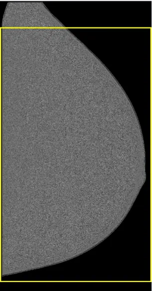
The algorithm has been adapted only in the final step of selection of the ROI where to perform the noise measure, in order to recognize in which side of the image the breast was positioned (laterality), and to take as ROI a rectangular region smaller than the FOV. The background pixel values inside this ROI are equal to 0 from both the digital imaging systems, so they can easily be ignored in the measurement of the
standard deviation. This was a fast way to implement the new ClinQC alternative version for a preliminary test, but the ROI includes also parts of the breast edges and skin where the noise might have different dependence on the body signal than inside the breast (the same happening for chest X-ray images), so the most correct way to implement this alternative version would be to select automatically a region that contains only the inner breast tissue and that has the same amount of pixels for all the analysed patient images.
Mammograms and tomosynthesis reconstructed projections can be generated from different exposures, but also different kVp, depending on the patients breast thick-nesses. This can introduce another source of variability on the noise measurement, that is not dependent on the imaging system quality and that for chest X-ray im-ages was irrelevant since only patient imim-ages acquired with 133 kV were used in this study. In this preliminary test all the images generated from both the imag-ing modalities mentioned before at different exposure levels and kVp were analysed together. The preliminary results are displayed in Section 3.2.2.2.
3.1.3
Validation of the ClinQC algorithm
In this Section, all the Methods developed for the validation of the ClinQC noise extraction algorithm are presented. A validation is the process that tests the algo-rithm under different conditions to see if its results are reproducible and dependent on the quality of the imaging system.
3.1.3.1 Image deterioration study
The first Method that has been invented in order to simulate a decrease or an increase in the quality of the imaging system is the image deterioration study. As explained in the Introduction (Section 2.3) the chest X-ray imaging systems can be really stable over long time periods, in fact there are no examples in the last years of a slow or fast quality degradation that we can use to verify if the ClinQC algorithm can detect it. So the only way to test if the algorithm is able to detect a deterioration of the imaging system is to deteriorate the quality of the images that it produces.
Two symmetrical approaches are presented.
3.1.3.1.1 Blur To blur the images is a way to reduce their amount of noise, so
the expected result of the test after blurring the images is to observe a decrease in their ClinQC noise values. If so, the decrease has to be significant to prove that the algorithm is sensitive to a change in the quality of the imaging system and in order to be recognized automatically with a detection algorithm. A reduction in the noise values could simulate an increase in the quality of the imaging system, that can occur if a new proper anti-scatter grid is installed for example (as can be observed in the examples in Section 3.2.1.3), or it can represent an increase in the exposure (mAs) given to the patients during the image acquisition. To verify if blurring the images is actually a way to simulate an increase of the exposure levels, a phantom study has been performed (Section 3.1.3.6).
The blurring study consists of smoothing at different levels different groups of im-ages, to run the ClinQC algorithm and to plot all the results in a time line. The increasing amount of blur was obtained linearly changing the σ of the Gaussian blurring kernel used to smooth the images, from σ = 0.5 pixel to σ = 2.05 pixel
(pixelsize = 0.12×0.12 mm). The first group consists of original unmodified images (instead of σ = 0 pixel). The sizes of the Gaussian blurring kernels varied
automati-cally with the values of σ, according to the law: kernel size = 2·ceil(2σ)+1 (pixel)2.
To study how the average noise value of the group of images changes, it is better not to use for every deterioration level the same group of images, but the approach used here was to randomly sub-sample different images every time. Instead, to study if and how the spread of the noise values changes, it is more meaningful to use the same group of images for each blurring level.
3.1.3.1.2 Gaussian noise The addition of noise to the images is done to observe
an increasing trend in the ClinQC noise values, that can occur when the detector or the electronics of the system reach their end of life, or if the anti-scatter grid is not present into its slot during the image acquisition (as can be observed in the examples in Section 3.2.1.3). An increase in the noise levels can simulate also a decrease in the dose (mAs) given to the patients. Different shapes of noise distributions can be added to the images to achieve different results: in the simulation presented in this thesis the symmetric distribution of Gaussian noise has been chosen to approximate the combined effect of all these deterioration phenomena in the most simple case. A different approach must be adopted in this case, since with this simulation we are changing something in the images that is exactly the quantity that we want to measure. So it would be a circular reasoning to add the same amount of noise to all the images and to measure if and how the ClinQC noise values change, since each image has a different initial level of noise. For example, two images A and B have
different σnoise A and σnoise B, if Gaussian noise with σnoise ADD is added to both
images, the ClinQC algorithm would register only a meaningless shift in the two
noise values, while their difference |σnoise B− σnoise A| would stay the same, since
the added noise is the same for both images. This inserts only a perturbation in the simulation result and does not give any new information on the extraction algorithm behaviour.
Instead, we don’t want to interfere in the measurement, but we want to add noise
2ceil = function that rounds to the nearest integer greater than or equal to the number in
only to simulate a controlled decrease in the quality of the imaging system. So the approach proposed here has the purpose to add different amounts of noise to the images according to their original estimated quality, and this is made possible by following three steps:
1) Estimate the original quality of each patient image by measuring its Signal to Noise Ratio (SNR). This can be made in two manners, the first one measures the SNR in decibel (dB) using the information from the entire image [15], the second one is more used in case the SNR of a single object or ROI in the image is measured:
SN Roriginal image = 10log10
σ2 original image σ2 noise image [dB] (3.2) SN Roriginal image =
µoriginal image (or ROI)
σnoise image (or ROI)
(3.3) where the noise image is the ClinQC high frequencies map, so the noise image extracted at the first step of the algorithm.
2) Choose the desired levels of deteriorations of the estimated SNR that have to be achieved by adding noise to the clinical images: linearly decreased percentages of the SNR, for example from 2% to 30%.
3) Use the inverse formula of Eq. 3.2, or Eq. 3.3, to compute the variance of the Gaussian noise with 0 mean that has to be added to the clinical image, with
an image processing tool (in this case MATLAB3), in order to achieve the desired
deterioration level of the estimated SNR.
σ2noise achieved= σ
2
original image
10SN Rdeteriorated10
[dB] (3.4)
But the additional step that avoids interfering in the measurement, as said be-fore, is to consider that each patient image has a different initial amount of noise. So the noise that has to be added to the image, in order to achieve the cho-sen level of deterioration of the SNR, must be reduced by the original amount of noise. Since these two amounts of noise are described by two distributions
with respective standard deviations σnoise added and σoriginal image, their addition
will result in a distribution with a standard deviation σnoise achieved that satisfies
σ2
noise achieved = σ2original image + σnoise added2 [16]. So the variance of the Gaussian
noise with 0 mean that has to be added to the image is: σnoise added2 = σ2
noise achieved− σ
2
original image (3.5)
Also in this case, to study how the average noise value of the group of images changes, the approach is to random sub-sample different images for each deterioration level. Instead, to study if and how the spread of the noise values changes, the same group of images has to be used.
3.1.3.2 Statistical analysis with simulations
This Section presents a statistical analysis regarding the stability of the ClinQC noise values performed by implementing two different types of simulations. These simulations are designed in order to produce output curves that answer the question: how many new clinical images have to be collected before an automated algorithm
can detect a step or a trend in the noise values with a certain significance level? So
we want to assess how fast is the response of the ClinQC algorithm to the simulated deterioration of the system, and how soon will the algorithm be able to provide an alarm, based on the noise level of each new clinical image acquired.
The purpose of the Step simulation (Section 3.1.3.2.1) is to detect a sharp breaking in the system that translates in a sudden change in the noise values from one patient to another. This can happen, for example, when the anti-scatter grid is replaced or removed (as can be observed in the examples in Section 3.2.1.3). While the Trend simulation provides different examples on the detection of the long term increase or decrease in the noise values.
Figure 3.7: Graphic reproduction of how a step in the noise values would appear.
3.1.3.2.1 Step simulation The general idea is to simulate a step in the noise
values (Fig. 3.7) with respect to the baseline (Section 3.2.1.2), and to understand how many clinical images are needed to detect it with a certain significance level. The following recipe explains the step simulation algorithm:
baseline dataset: µ, σ, skewness and kurtosis (Section 3.2.1.2).
2) Increase the baseline mean (µbaseline) with a different increasing factor at every
loop.
(example: µsimulated = µbaseline· increasing factor, where the increasing factors are num-bers like 1.03, 1.15, . . . , that indicate an increase of 3%, 15%, . . . )
3) Use each new increased mean µsimulated, with the original other parameters that
characterize the distribution of the ClinQC noise values baseline dataset σ, skewness and kurtosis, to simulate from the same designed distribution new groups of noise values of increasing sizes: for each loop (so for each new simulated mean) generate M (very high) new datasets of each size.
(example: µsimulated 1 = 0.0060 (baseline mean increased by 3%)
1st new dataset (size = 2 noise values) → [0.00596 , 0.00633] → ×M iterations
2nd new dataset (size = 3 noise values)→ [0.00591 , 0.00594 , 0.00621] → ×M iterations . . .
Nth new dataset (size = N+1 noise values) → [0.00628 , 0.00605 , . . . , 0.00594] → ×M iterations.)
4) For each one of the new N·M datasets of simulated groups of noise values of
different sizes, perform an unpaired T-test to test the null hypothesis that the sim-ulated datasets come from normal distributions with the same mean and equal but unknown variance as the baseline of the ClinQC noise values.
In some cases, especially when small sizes of the noise values groups are simulated, it is possible that the T-test cannot reject the null hypothesis based on so small datasets. That is why M iterations are required: in this way the rejection ratio of T-test for each one of the new dataset sizes is
Rejection Ratio= number of times the null hypothesis is rejected
M total T − tests (iterations) . (3.6)
A plot of how the Rejection Ratio varies with the different sizes of the simulated datasets indicates the scoring of the T-test in detecting a change in the noise values, when a certain number of new images produces noise values distributed with a mean higher than the baseline. This results in a diagram with similar meaning and shape as a ROC [17].
5) Now if a threshold is chosen in the y-axis of the Rejection Ratio representation, for example at 99.5%, the first integer size of the simulated datasets that exceeds
the threshold in the rejection ratio curve is the minimum number of images that we need to say, with a high level of certainty, that the mean of the simulated noise values is actually higher than the baseline, and that the two distributions can be considered unequal.
6) If this analysis is done for each one of the increasing factors for the baseline mean,
so for each different µsimulated, it is possible to find the minimum number of images
to reject the null hypothesis in function of the baseline increase in percentage: and this is the curve that answers the original question (how many new clinical images have to be collected before an automated algorithm can detect a step or a trend in
the noise values with a certain significance level?).
If the question is less general, in particular if the user wants to know how many images are needed to detect a step exactly like the one produced by a known effect like the anti-scatter grid removal or replacement (history examples shown in Section 3.2.1.3), the step simulation can be adapted for this purpose. In this specific case, there is no need to simulate many baseline increases, since the difference between
µbaseline and µN O grid or µOLD grid in percentage is already known (Section 3.2.1.3).
So the Rejection Ratio with the proper threshold already tells the user how many images are needed to detect the expected step in a specific occasion.
Figure 3.8: Graphic reproduction of how a trend in the noise values would appear.
3.1.3.2.2 Trend simulation The trend simulation, instead, generates a slope
(Fig. 3.8) is detected.
1) Find the parameters that describe the distribution of the ClinQC noise values baseline dataset: µ, σ, skewness and kurtosis (Section 3.2.1.2).
2) Generate new baseline values from the same distribution described with the parameters found at step 1.
3) Generate new noise values from the same distribution arranged in a slope and align them to the baseline data points simulated at step 2. The number of simulated points represents a specific time line (like one week or one month of patients exams), while the slope reflects the strength of the simulated deterioration occurring in the imaging system.
4) Choose different sizes of a moving window, that can be dragged point-by-point on the simulated slope of noise values in order to perform series of unpaired T-test, between the average value of the simulated noise values that fall inside the moving window and the baseline distribution of the ClinQC noise values.
5) Each time the moving window of a chosen size is shifted, the T-test scoring is recorded and normalized by the total number of iterations. This results in the Rejection Ratio (Eq. 3.6) that can be plotted against the position in the slope when the alarm is produced.
6) Then a similar approach used in the step simulation (point 5) is adopted: a threshold of 99.5% in the Rejection Ratio plot specifies the percentage of increase of the baseline on the slope where the T-test has been able to reveal a change in the noise values in at least the 99.5% of the iterations.
7) If points 4, 5 and 6 are repeated for different sizes of the moving window, the final curve of the trend simulation can be obtained by plotting the percentage of increase of the baseline simulated by the slope, against the size of the window that was able to detect it. The most important difference between the two simulations presented in this Section is that the Trend simulation curve is dependent on the chosen time line and strength of the slope, but both simulations give curves that indicate the detectability of different conditions by using the ClinQC algorithm.
3.1.3.3 The ClinQC performance in clinical practice How would the ClinQC noise algorithm work in clinical practice?
The stable history of the imaging system, monitored with the QClight phantom analysis, shows the device is in good health. During routine clinical use the anti-scatter grid was unintendedly inserted facing the wrong direction. This was detected during the QClight measurement the next Monday morning in July 2016. The QClight images acquired during the weekly QC were extremely inhomogeneous but symmetrical along the vertical axis. The noise measurement was lower than the average QClight baseline. The medical physicists hypothesized that the anti-scatter grid had been flipped, this was confirmed after a manual check on the imaging system.
But when exactly did it happen during the previous week? This very specific answer can’t be given by a weekly QC as the QClight. So here is where the performance of the ClinQC algorithm has been tested on an actual problem of the imaging system. It has been possible to observe and study the effects of this human mistake using the ClinQC algorithm and this became an important part of its validation.
All the clinical images acquired with the X-ray imaging system during the two weeks when the problem was identified with the QClight analysis were extracted from the PACS. The ClinQC noise extraction algorithm was run on all the images producing values that fell within the range of acceptance defined by the baseline limits, while a clearly visible step down in the noise values and up in the exposure levels was observed in almost three complete days. Since the noise values after the step differ from the baseline of a certain percentage that has been measured in Section 3.2.5, according to the Step simulation output curve (Fig. 3.2.4.1), the minimum size of the moving window that can be used to detect the step in the noise values is defined. All these results and procedures are illustrated in Section 3.2.5.
3.1.3.4 Outlier analysis
The analysis of the outlier noise values produced by the ClinQC algorithm is useful to understand if there are specific categories of patients that are more susceptible to produce outliers. All the images acquired after the update of the anti-scatter grid by the end of 2014, extracted from the PACS during my thesis internship, were
the input of the ClinQC algorithm and their noise values were compared to the ClinQC baseline. First of all, a correlation between the ClinQC noise outliers and the exposure outliers was investigated. Second, the sex of the outliers was compared to the percentage of males and females undergoing a chest X-ray examination. It was not possible to compare the histogram of ages of the outliers to the distribution of ages of all the patients of one year, since it would have meant to extract more than 300 GB of additional images from the PACS archive to retrieve patient ages from their DICOM tags and draw the annual age distribution of patients in the examined imaging system. For the same reason it was not possible to study the presence in the noise outliers of patients with nodules or sharp objects in the chest area, since an automated search algorithm for these structures would have needed to run not only in the already available images but also in the annual dataset of images that was not possible to extract, in order to establish a statistical correlation.
3.1.3.5 Image Pyramids noise extraction algorithm comparison
The image Pyramids are a multi-scale representation of an image which is subject to repeated smoothing, sub-sampling and/or other manipulations. They are now widely used for image compression, object recognition and multi-scale analysis, but also for noise extraction from clinical images [18]. This last approach uses a Lapla-cian pyramid to decompose the chest images into many digressive spatial frequency sub-bands, in order to separate the high frequencies (mainly noise) from the low frequencies (mainly anatomical signal). A Gaussian pyramid is formed by an image
G0 that is subsequently filtered with average blurring kernels and downscaled many
times (first line of the example Fig. 3.9). All the images of the Gi series (with i
= 0 . . . Nlevels of the Pyramid) can then be up-sampled back to the original size,
observing an increasing smoothed appearance (second line, Fig. 3.9). The Laplacian Pyramid [19] stores the differences pixel-by-pixel of the images at each adjacent stage
of the Gaussian Pyramid Li = Gi − Gi−1, obtaining many residuals images (third
line, Fig. 3.9). The first stage of the Laplacian Pyramid L1 = G1− G0 (original image)
will show mainly the noise information, while at higher levels the noise will be grad-ually replaced by the low frequency coarse structures.
The ClinQC noise extraction algorithm and the Pyramids method are based on the same ideas, while the implementation is different. In fact to achieve the extraction of a noise map from a clinical image both methods combine a smoothing and a subtraction. The additional step that only the ClinQC algorithm includes is a normalization by the low frequencies image.
A comparison between these two methods has been performed using the clinical images forming the baseline dataset Section 3.2.1.2. The Laplacian Pyramid at the first stage was used as the ClinQC noise map taking a square ROI in the center and measuring a not normalized noise value but, to better compare the noise values
produced by the two methods, the Laplacian Pyramid at the first stage L1 has been
also normalized by the corresponding low frequencies stage G1. The results are
G1 L1 G2 L2 G3 L3 G4 L4 G5 L5
Figure 3.9: Example of Gaussian and Laplacian Pyramids.
3.1.3.6 Phantom comparisons
The ClinQC algorithm for noise extraction has been validated performing also a phantom comparison study. The two phantoms available at LUMC for this purpose
were the QClight copper plate (Section 2.2) and RANDO4 anthropomorphic chest
phantom, representing the skull and trunk of a 175 cm tall male weighing 73.5 kg (Fig. 3.10).
In order to establish if the ClinQC is a reliable algorithm to extract and measure noise from clinical images, a correlation between this new patient-based approach and the QClight phantom-based method has been investigated: the patient-based technique was simulated by applying the ClinQC algorithm to RANDO anthro-pomorphic phantom images, acquired with the same protocol used for patients at different exposures (since images at different exposure levels of the same patient were not available). The QClight images were acquired within the same range of
Figure 3.10: RANDO anthropomorphic phantom.
mAs, using both the phantom and the patient acquisition protocols.
The QClight noise data, saved each Monday during the history of the imaging sys-tem with the actual setting, have been compared with the ClinQC noise value of one clinical image per week in the same time line. In this case, only the CoV of the noise values obtained with the two methods have been compared, while the correlation was not expected to be observed, since both the clinical and the phantom images are acquired at approximately constant exposures.
The final test that was performed using phantoms was to confirm the findings of the image deterioration study using blurring deterioration. In fact, the test was implemented in order to investigate if blurring the images is the correct way to sim-ulate an increase of the mAs, in addition to a noise decrease that can be observed in Section 3.2.3.1. The same images of RANDO and QClight, previously acquired us-ing, respectively, patient and phantom acquisition protocols at different exposures,
were used. The images acquired at 1.6 mAs were blurred applying filters with differ-ent increasing sigma of Gaussian blurring kernels. The resulting noise values were computed using the ClinQC algorithm for RANDO images, and with the original method for the QClight images. The dependency of the noise on the exposure and blur setting were compared by plotting the resulting noise values together in one figure.
The 2D Noise Power Spectrum (NPS) of the images obtained at different exposures and after each blurring deterioration are also displayed to compare the effect of mAs and blurring on the noise frequencies.