Alma Mater Studiorum – Università di Bologna
FACOLTÀ DI INGEGNERIA
CORSO DI LAUREA IN CIVIL ENGINEERING
Tesi di laurea in
ADVANCED DESIGN OF STRUCTURES
Interaction between Axial Force, Shear and Bending
Moment in Reinforced Concrete Elements
Candidato: Relatore: GIULIA CASTORI Prof. Ing. STEFANO SILVESTRI
Correlatore: Prof. Ing. TOMASO TROMBETTI Dott. Ing. MICHELE PALERMO
Sessione III
2
Abstract
Il collasso di diverse colonne, caratterizzate da danneggiamenti simili, quali ampie fessure fortemente inclinate ad entrambe le estremità dell’elemento, lo schiacciamento del calcestruzzo e l’instabilità dei ferri longitudinali, ha portato ad interrogarsi riguardo gli effetti dell’interazione tra lo sforzo normale, il taglio ed il momento flettente.
Lo studio è iniziato con una ricerca bibliografica che ha evidenziato una sostanziale carenza nella trattazione dell’argomento.
Il problema è stato approcciato attraverso una ricerca di formule della scienza delle costruzioni, allo scopo di mettere in relazione lo sforzo assiale, il taglio ed il momento; la ricerca si è principalmente concentrata sulla teoria di Mohr.
In un primo momento è stata considerata l’interazione tra solo due componenti di sollecitazione: sforzo assiale e taglio. L’analisi ha condotto alla costruzione di un dominio elastico di taglio e sforzo assiale che, confrontato con il dominio della Modified Compression Field Theory, trovata tramite ricerca bibliografica, ha permesso di concludere che i risultati sono assolutamente paragonabili. L’analisi si è poi orientata verso l’interazione tra sforzo assiale, taglio e momento flettente. Imponendo due criteri di rottura, il raggiungimento della resistenza a trazione ed a compressione del calcestruzzo, inserendo le componenti di sollecitazione tramite le formule di Navier e Jourawsky, sono state definite due formule che mettono in relazione le tre azioni e che, implementate nel software Matlab, hanno permesso la costruzione di un dominio tridimensionale. In questo caso non è stato possibile confrontare i risultati, non avendo la ricerca bibliografica mostrato niente di paragonabile.
Lo studio si è poi concentrato sullo sviluppo di una procedura che tenta di analizzare il comportamento di una sezione sottoposta a sforzo normale, taglio e momento: è stato sviluppato un modello a fibre della sezione nel tentativo di condurre un calcolo non lineare, corrispondente ad una sequenza di analisi lineari.
4
Table of Contents
1. Literature Review ... 10 1.1. Analytical Articles ... 10 1.1.1. Article 1 ... 10 1.1.2. Article 2 ... 13 1.1.3. Article 3 ... 15 1.1.4. Article 4 ... 17 1.1.5. Article 5 ... 19 1.1.6. Article 6 ... 21 1.2. Numerical Researches ... 23 1.2.1. Article 7 ... 23 1.2.2. Article 8 ... 25 1.2.3. Article 9 ... 27 1.2.4. Article 10 ... 29 1.3. Experimental Studies ... 31 1.3.1. Article 11 ... 31 1.3.2. Article 12 ... 33 1.3.3. Article 13 ... 352. The Modified Compression Field Theory ... 38
2.1. Theoretical Approach ... 38
2.1.1. Introduction ... 38
2.1.2. Compatibility Conditions ... 39
2.1.3. Equilibrium Conditions ... 40
2.1.4. Constitutive Laws ... 41
2.1.5. Average Stress-Average Strain Response of Concrete ... 42
2.1.6. Transmitting Loads across Cracks ... 42
2.2. Implementation of the MCFT ... 44
2.2.1. Problem Definition ... 44
2.2.2. Input Data ... 45
5
2.2.3.1. First Iteration... 45
2.2.3.2. Following Iterations ... 49
2.3. N.T Interaction Domain based on MFCT ... 49
3. Mohr’s Theory to Construct the Interaction Domains ... 52
3.1. Construction of N-T Domain ... 52
3.1.1. Matlab Implementation ... 55
3.1.1.1. Problem Definition ... 55
3.1.1.2. Formulae Implementation ... 56
3.1.2. Construction of the N-T domain for a Real Column ... 57
3.2. Construction of N-T-M Domain ... 59
3.2.1. Stress-Block distribution of Normal Stresses due to Bending ... 59
3.2.1.1. Half Cross-Section Subjected to Traction Force related to the Moment ... 60
3.2.1.2. Half Cross-Section Subjected to Compression Force related to the Moment ... 64
3.2.1.3. Matlab Implementation ... 68
3.2.1.4. Problem Definition ... 68
3.2.1.5. Formulae Implementation ... 69
3.2.2. Linear Distribution of Normal Stresses due to Bending ... 70
3.2.2.1. Hypotheses ... 71
3.2.2.2. Navier’s Formula ... 71
3.2.2.3. Jourawsky’s Equation ... 72
3.2.2.4. Failure Criteria ... 72
3.2.2.4.1. Achievement of the Tensile Strength of the Concrete ... 73
3.2.2.4.2. Achievement of the Compressive Strength of the Concrete ... 74
3.2.2.4.3. Achievement of the Tensile Strength of the Steel ... 76
3.2.2.4.4. Achievement of the Compressive Strength of the Steel ... 76
3.2.2.5. Discretization of the Cross Section ... 77
3.2.2.5.1. Main Quantities Definition... 77
3.2.2.5.2. Effect of the Axial Force not applied in the Centroid ... 79
3.2.2.5.3. Stirrups Contribution ... 80
3.2.2.6. Matlab Implementation ... 83
6
3.2.2.6.2. Discretization of the cross section ... 84
3.2.2.6.3. Main Quantities Definition... 85
3.2.2.6.4. Moment Vector ... 86
3.2.2.6.5. Shear Vector ... 87
3.2.2.6.6. Construction of the Domain ... 87
3.2.2.6.7. Domains Refinement ... 88
3.2.2.6.8. Plot of the Domain... 89
4. Nonlinear Evaluation of the Cross Section as a Sequence of Linear Analyses ... 92
4.1. Basic Quantities Definition ... 93
4.2. Hypotheses ... 94
4.3. Evaluation of Normal Stresses Distribution on the Cross-Section ... 95
4.4. Evaluation of Tangential Stresses Distribution on the Cross-Section ... 96
4.5. Analysis of the Condition of the Cross Section ... 97
5. Suggested Procedure ... 100
5.1. Input Data ... 101
5.2. Elastic Evaluation of the Cross Section ... 102
5.2.1. Basic Quantities Evaluation ... 102
5.2.2. Normal Stresses Distribution ... 103
5.2.3. Tangential Stresses Diagram ... 104
5.3. Possible Alternative Scenarios ... 105
5.3.1. First Scenario ... 107 5.3.2. Second Scenario ... 108 5.3.3. Third Scenario ... 109 5.3.4. Fourth Scenario ... 110 5.3.5. Fifth Scenario ... 113 5.3.6. Sixth Scenario ... 114 6. Applicative Examples ... 116
6.1. Practical Example of the Fourth Scenario ... 116
6.1.1. Input Data ... 116
6.1.2. 1st Elastic Evaluation of the Cross Section ... 117
7
6.1.2.2. Normal Stresses Distribution... 119
6.1.2.3. Tangential Stress Distribution ... 120
6.1.2.4. Principal Stresses ... 121
6.1.3. 2nd Elastic Evaluation of the Cross Section ... 122
6.1.4. 3rd Elastic Evaluation of the Cross Section ... 125
6.1.5. 4th Elastic Evaluation of the Cross Section ... 127
6.1.6. 5th Elastic Evaluation of the Cross Section ... 129
6.2. Practical Example of the Fifth Scenario ... 133
6.2.1. Input Data ... 133
6.2.2. 1st Elastic Evaluation of the Cross Section ... 134
6.2.3. 2nd Elastic Evaluation of the Cross Section ... 137
6.2.4. 3rd Elastic Evaluation of the Cross Section ... 140
6.3. Practical Example of the Sixth Scenario... 145
6.3.1. Input Data ... 145
6.3.2. 1st Elastic Evaluation of the Cross Section ... 146
6.3.3. 2nd Elastic Evaluation of the Cross Section ... 149
6.3.4. 3rd Elastic Evaluation of the Cross Section ... 152
6.3.5. 4th Elastic Evaluation of the Cross Section ... 154
6.4. Application of the Procedure to Real Cases ... 158
6.4.1. Case 1 ... 158
6.4.1.1. 1st Elastic Evaluation of the Cross Section ... 160
6.4.2. Case 2 ... 164
6.4.2.1. 1st Elastic Evaluation of the Cross Section ... 165
6.4.2.2. 2nd Elastic Evaluation of the Cross Section ... 168
6.4.2.3. 3rd Elastic Evaluation of the Cross Section ... 170
6.4.2.4. 4th Elastic Evaluation of the Cross Section ... 172
6.4.2.5. 5th Elastic Evaluation of the Cross Section ... 174
6.4.2.6. 6th Elastic Evaluation of the Cross Section ... 175
6.4.2.7. 7th Elastic Evaluation of the Cross Section ... 176
6.4.2.8. 8th Elastic Evaluation of the Cross Section ... 178
8
5.4.2.10 10th Elastic Evaluation of the Cross Section ... 180
6.4.3. Case 3 ... 182
6.4.3.1. 1st Elastic Evaluation of the Cross Section ... 184
6.4.3.2. 2nd Elastic Evaluation of the Cross Section ... 186
6.4.3.3. 3rd Elastic Evaluation of the Cross Section ... 189
6.4.3.4. 4th Elastic Evaluation of the Cross Section ... 191
7. Design of the Laboratory Test ... 196
8. Conclusions... 198
10
1. Literature Review
The study begun with a literature review in order to analyse how other researchers approached the problem. Many articles examined, only most important have reported. They divide into analytical, numerical and experimental articles.
1.1. Analytical Articles
1.1.1. Article 1
Authors: Frank J. Vecchio and Michael P. Collins Journal: ACI Structural Journal, 1986
Title: The Modified Compression-Field Theory for Reinforced Concrete Elements Subjected to Shear Focus of Research
The article presents an analytical model capable of predicting the load-deformation response of reinforced concrete elements subjected to in-plane shear and normal stresses. In the model, cracked concrete is treated as a new material with its own stress-strain characteristics. Equilibrium, compatibility, and stress-strain relationships are formulated in terms of average stresses and average strains. Consideration is also given to local stress conditions at crack locations. The stress-strain relationships for the cracked concrete were determined testing 30 RC panels.
11
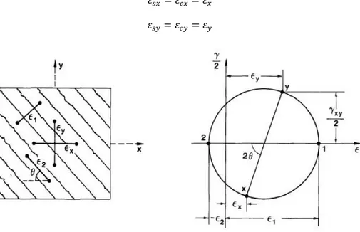
The membrane element considered is a portion of a reinforced concrete structure, containing an orthogonal grid of reinforcement with the longitudinal, x,and transverse, y,axes coincident with the reinforcement directions. Loads applied consist of uniform axial stresses 𝑓𝑥 and 𝑓𝑦, and uniform
shear stress 𝜈𝑥𝑦. The problem is to determine how the three in-plane stresses 𝑓𝑥
,
𝑓𝑦, and 𝜈𝑥𝑦 arerelated to the three in-plane strains 𝜀𝑥, 𝜀𝑦 and 𝛾𝑥𝑦. Assuming that concrete and steel bars are perfectly
bonded together corresponds to: 𝜀𝑠𝑥= 𝜀𝑐𝑥= 𝜀𝑥 and 𝜀𝑠𝑦= 𝜀𝑐𝑦= 𝜀𝑦. If 𝜀𝑥, 𝜀𝑦 and 𝛾𝑥𝑦 are known, then the
strain in any other direction can be obtained from the Mohr's circle of strain: 𝛾𝑥𝑦= 2(𝜀1−𝜀2) tan 𝜃 where 𝜀𝑥+ 𝜀𝑦= 𝜀1+ 𝜀2 and 𝑡𝑎𝑛2𝜃 = 𝜀𝑥−𝜀2 𝜀𝑦−𝜀2= 𝜀1−𝜀𝑦 𝜀1−𝜀𝑥= 𝜀1−𝜀𝑦 𝜀𝑦−𝜀2 = 𝜀𝑥−𝜀2 𝜀1−𝜀𝑥.
The forces applied to the reinforced concrete element are carried by stresses in the concrete and in the reinforcement. The requirement that forces sum to zero in the x-direction corresponds to: ∫ 𝑓𝐴 𝑥𝑑𝐴= ∫ 𝑓𝐴𝑐 𝑐𝑥𝑑𝐴𝑐+ ∫ 𝑓𝐴𝑠 𝑠𝑥𝑑𝐴𝑠, which is 𝑓𝑥= 𝑓𝑐𝑥+ 𝜌𝑠𝑥∗ 𝑓𝑠𝑥. The following equilibrium conditions:
𝑓𝑦= 𝑓𝑐𝑦+ 𝜌𝑠𝑦∗ 𝑓𝑠𝑦, 𝜈𝑥𝑦= 𝜈𝑐𝑥+ 𝜌𝑠𝑥∗ 𝜈𝑠𝑥, 𝜈𝑥𝑦= 𝜈𝑐𝑦+ 𝜌𝑠𝑦∗ 𝜈𝑠𝑦. Assuming 𝜈𝑐𝑥= 𝜈𝑐𝑦 = 𝜈𝑦𝑥, stresses in
concrete are defined: 𝑓𝑐𝑥= 𝑓𝑐1− 𝜈𝑐𝑥/ tan 𝜃𝑐, 𝑓𝑐𝑦= 𝑓𝑐1− 𝜈𝑐𝑥∗ tan 𝜃𝑐.
Constitutive relationships to link average stresses to average strains for reinforcement and concrete: 𝑓𝑠𝑥= 𝐸𝑠∗ 𝜀𝑥≤ 𝑓𝑥𝑦, 𝑓𝑠𝑦= 𝐸𝑠∗ 𝜀𝑦≤ 𝑓𝑥𝑦 and 𝜈𝑠𝑥= 𝜈𝑠𝑦= 0. Concerning the concrete, principal
stress axes and principal strain axes assume coincident: 𝜃𝑐= 𝜃.
Thanks to experimental tests was found that principal compressive stress in the concrete, 𝑓𝑐2, was a
function, not only of the principalcompressive strain, 𝜀2, but also of the co-existing principaltensile
strain, 𝜀1• The relationship suggested is: 𝑓𝑐2= 𝑓𝑐2,𝑚𝑎𝑥∗ [2 ( 𝜀2 𝜀𝑐′) − ( 𝜀2 𝜀𝑐′) 2 ] where 𝑓𝑐2,𝑚𝑎𝑥 𝑓′𝑐 = 1 0.8−0.34𝜀1 𝜀𝑐′ ≤ 1.
Concerning the average principal tensile stress in the concrete, prior cracking 𝑓𝑐1 = 𝐸𝑐∗ 𝜀1, after 𝑓𝑐1 = 𝑓𝑐𝑟
1+√200𝜀1. The stresses and strains formulations described deal with average values and do not give
information about local variation. At a crack, there are no average conditions.
As the applied external stresses 𝑓𝑥
,
𝑓𝑦, and 𝜈𝑥𝑦 are fixed, the internal stresses must be staticallyequivalent: 𝜌𝑠𝑥𝑓𝑠𝑥sin 𝜃 + 𝑓𝑐1sin 𝜃 = 𝜌𝑠𝑥𝑓𝑠𝑥𝑐𝑟sin 𝜃 − 𝑓𝑐𝑖sin 𝜃 − 𝜈𝑐𝑖cos 𝜃; the same in y
direction: 𝜌𝑠𝑦𝑓𝑠𝑦cos 𝜃 + 𝑓𝑐1cos 𝜃 = 𝜌𝑠𝑦𝑓𝑠𝑦𝑐𝑟cos 𝜃 − 𝑓𝑐𝑖cos 𝜃 − 𝜈𝑐𝑖sin 𝜃. The two equilibrium equations can
be satisfied with no shear and compression stresses on the crack, which means: 𝜌𝑠𝑦(𝑓𝑠𝑦𝑐𝑟− 𝑓𝑠𝑦) =
𝜌𝑠𝑥(𝑓𝑠𝑥𝑐𝑟− 𝑓𝑠𝑥) = 𝑓𝑐1. However, the stress in the reinforcement at a crack cannot exceed the yield
strength, that is: 𝑓𝑠𝑥𝑐𝑟 ≤ 𝑓𝑠𝑥, 𝑓𝑠𝑦𝑐𝑟 ≤ 𝑓𝑠𝑦. If the calculated average stress in reinforcement is high, it may
not be possible to satisfy the equilibrium. In this case, equilibrium will require shear stresses on the crack. The relationship between the shear on the crack 𝜈𝑐𝑖, the crack width wand the compressive
stress on the crack 𝑓𝑐𝑖 has experimentally studied, Walraven formula is: 𝜈𝑐𝑖 = 0.18 𝜈𝑐𝑖,𝑚𝑎𝑥+ 1.64 𝑓𝑐𝑖−
0.82 𝑓𝑐𝑖2
𝜈𝑐𝑖,𝑚𝑎𝑥, 𝜈𝑐𝑖,𝑚𝑎𝑥=
√−𝑓𝑐′ 0.31+24 𝑤 (𝑎+16)⁄ .
12 Obtained Results
The MCFT is a powerful analytical tool, but is simple enough to be programmed with a handheld calculator. Not only is it capable of predicting the test results reported in this paper, but it has used by other researchers to successfully predict their test results.
13
1.1.2. Article 2
Authors: Michael P. Collins, Denis Mitchell, Perry Adebar, and Frank J. Vecchio Journal: ACI Structural Journal, 1996
Title: A General Shear Design Method Focus of Research
The objective of this paper is to briefly present a simple, general shear design method based on the Modified Compression Field Theory, MCFT.
The principal compressive stress in the concrete, 𝑓2, relates to both principal compressive and tensile
strain, 𝜀1 and 𝜀2: 𝑓2= 𝑓2,𝑚𝑎𝑥[ 2𝜀2 𝜀′𝑐− ( 𝜀2 𝜀′𝑐) 2 ], where 𝑓2,𝑚𝑎𝑥= 𝑓′𝑐 0.8+170 𝜀1 ≤ 𝑓 ′
𝑐. From the first equation
derives 𝜀2= −0.002 (1 − √1 − 𝑓2
𝑓2,𝑚𝑎𝑥). After cracking: 𝑓1= 𝑓𝑐𝑟
1+√500 𝜀1, with 𝑓𝑐𝑟= 4√𝑓′𝑐. For large values
of 𝜀1, cracks become wide, the magnitude of 𝑓1is governed by the yielding of reinforcement at crack
and by the ability to transmit shear stresses, 𝜈𝑐𝑖, across the interface, which is a function of the crack
width, 𝑤, and the aggregate size, 𝑎: 𝜈𝑐𝑖 = 0.18 √𝑓′𝑐 0.3+24 𝑤 𝑎+16
. Is stirrups have reached their yielding stress and crack begins to slip, the average tensile stress in the concrete, 𝑓1 = 𝜈𝑐𝑖 𝑡𝑎𝑛𝜃.
Figure 1.1.2.1 – Approach of GSM
For the design, 𝜀𝑥, the highest longitudinal strain occurring within the web, can be approximated as
the strain in the flexural tension reinforcement: 0 ≤ 𝜀𝑥= (𝑀𝑢
𝑑𝑣)+0.5 𝑁𝑢+0.5 𝑉𝑢 𝑐𝑜𝑡𝜃−𝐴𝑝𝑠 𝑓𝑝𝑜
𝐸𝑠 𝐴𝑠+𝐸𝑝 𝐴𝑝 ≤ 0.002. From
strain compatibility: 𝜀1= 𝜀𝑥+ (𝜀𝑥− 𝜀2) 𝑐𝑜𝑡2𝜃; hence, as longitudinal strain, 𝜀𝑥, increases and the
inclination of principal compressive stress, 𝜃, reduces, the “damage indicator”, 𝜀1, increases. The
nominal strength of a member 𝑉𝑛= 𝑉𝑐+ 𝑉𝑠+ 𝑉𝑝= 𝑓1 𝑏𝑣 𝑑𝑣cot 𝜃 + 𝐴𝑣 𝑓𝑦
𝑠 𝑑𝑣cot 𝜃 + 𝑉𝑝= 𝛽√𝑓′𝑐 𝑏𝑣 𝑑𝑣+ 𝐴𝑣 𝑓𝑦
𝑠 𝑑𝑣cot 𝜃 + 𝑉𝑝, where tensile stress factor 𝛽 =
0.33 cot 𝜃 1+√500 𝜀1≤
0.18 0.3+24 𝑤
𝑎+16
, 𝑤 = 𝑠 𝜀1. The value of principal
14
strain, 𝜀2, which can be computed through equation, defined above, imposing 𝑓2= ( 𝑉𝑛−𝑉𝑝
𝑏𝑣 𝑑𝑣) (tan 𝜃 +
cot 𝜃).
Using the relationship above: 𝜀1= 𝜀𝑥+ [𝜀𝑥+ 0.002 (1 − √1 − 𝜈 𝑓′ 𝑐
(tan 𝜃 + cot 𝜃) ( 0.8 + 170𝜀1))] 𝑐𝑜𝑡2𝜃.
The amount of shear reinforcement must satisfy 𝑉𝑠≥ 𝑉𝑢
𝜑 − 𝑉𝑐− 𝑉𝑝, where 𝑉𝑢≤ 𝜑 𝑉𝑛.
The shear influences the tensile forces in longitudinal reinforcement. At the inner edge of the bearing area, the tensile force has to be: 𝑇 = (𝑉𝑢
𝜑− 0.5 𝑉𝑠) cot 𝜃. This equation gives additional tension
due to shear, and therefore, at a section subjected to shear, 𝑉𝑢, a moment, 𝑀𝑢, and an axial force, 𝑁𝑢,
longitudinal bars on the flexural tension side of the element must satisfy: 𝐴𝑠 𝑓𝑦+ 𝐴𝑝𝑠 𝑓𝑝𝑠≥ 𝑀𝑢 𝜑 𝑑𝑣+ 0.5 𝑁𝑢 𝜑 + ( 𝑉𝑢 𝜑− 0.5 𝑉𝑠− 𝑉𝑝) cot 𝜃.
The general equation of the MCFT, intended to account for the complex behaviour of diagonally cracked concrete, are more suited for computer solution, like RESPONSE-2000, than for hand calculation. With tables of 𝜃 and 𝛽, the method becomes simple enough to solve by hand. For the design. Using formulae mentioned above, the steps are the following:
1. At the design section, calculate the shear stress 𝜈; 2. Calculate the longitudinal strain 𝜀𝑥;
3. Choose the values of 𝜃 and 𝛽 4. Determine the nominal strength;
5. Check the capacity of longitudinal reinforcement. Obtained Results
This approach has verified through experimental tests. 528 specimens were tested and as many shear failures resulted. Those failures were compared to the failure shear predicted by the method presented in this paper. The proposed General Method predicts the failure shears more accurately than those given by the ACI code do. A key feature of this procedure is the explicit consideration of the influence of shear upon longitudinal reinforcement, aspect that could avoid serious errors.
15
1.1.3. Article 3
Authors: M.J. Nigel Priestley, Ravindra Verma, and Yan Xiao Journal: Journal of Engineering Mechanics, 1999
Title: Seismic Shear Strength of Reinforced Concrete Columns Focus of Research
This paper examines a number of methods to predict shear strength of columns and compares the results with existing database. A refinement and simplification of the method developed by Ang et al. (1989) and Wong et al. (1993) is proposed, which results in close agreement between predicted and measured shear strength over the full range of experimental database.
The ASCE/ACI 426 approach does not consider the influence of ductility; the Ang-Wong model work well in low ductility, but scatter increases at moderate to high ductility levels, apparently as a consequence of the residual shear strength, being assumed independent of the axial load level and the aspect ratio. The Watanabe-Ichinose approach provides good prediction for rectangular columns at low axial load levels, the lack of specific consideration about axial loads leads to increased conservatism as the axial load level increases. In this model, for ductile shear strength, the strength of both arch and truss mechanisms are reduced. Experimental data indicate a reduction in the inclination of diagonal cracking to the column axis as the ductility increases, implying an increase in the truss mechanism.
The proposed equation bases on the formulation given by Ang and Wong. The shear strength of a column is supposed to consist of three independent components: a concrete component, 𝑉𝑐, whose
magnitude depends on the level of ductility, an axial load component, 𝑉𝑝, depending on the column
aspect ratio, and a truss component, 𝑉𝑠, function of transverse reinforcement: 𝑉𝑛= 𝑉𝑐+ 𝑉𝑝+ 𝑉𝑠. The
concrete term reduces with increasing ductility: 𝑉𝑐= 𝑘 √𝑓′𝑐 𝐴𝑐, where 𝑘 depends on the member
displacement ductility level, on the system of unit used and whether the column is subjected to uniaxial or biaxial ductility demand; the effective shear area, 𝐴𝑐= 0.8 𝐴𝑔𝑟𝑜𝑠𝑠.
It is considered that the column axial force enhance the shear strength by arch action and inclined strut. In this approach, the arch action only depends on the axial load level. The enhancement of the shear strength relates to the horizontal component of the diagonal compression strut, since this component directly resists the applied force. Thus: 𝑉𝑝= 𝑃 tan 𝛼 =
𝐷−𝑐
2𝑎 𝑃, where 𝐷 is the overall section
depth or diameter, 𝑐 the depth of the compression zone, 𝑎 = 𝐿 for cantilever columns and 𝑎 =𝐿
2 for
column in reversed bending.
The contribution of transverse reinforcement to shear strength bases on truss mechanism using 30° angle between the compression diagonals, the crack pattern, and the column axis. For rectangular column: 𝑉𝑠 =
𝜋 2
𝐴𝑠ℎ 𝑓𝑦ℎ 𝐷′
𝑆 cot 30°, where 𝐷′ is the distance between centres of the peripheral hoops or
16
Figure 1.1.3.1 – Equations compared to experimental results
Obtained Results
Results reported in the figure indicates a greatly improvement prediction. The influence of ductility, axial load and aspect ratio appear to be well represented by the proposed method. With respect to the methods discussed at the beginning, the model proposed in this paper provides the closest agreement with the data, with a mean strength ratio of 1.021 and a standard deviation of 0.124. This standard deviation is less than 40% of that resulting from the ASCE/ACI 426 and Watanabe-Ichinose, and 61% than Ang-Wong model.
It could be argued that the proposed method is a predictive equation, whereas the alternative ones are design equations. Consequently, higher values of the strength ratio are desirable. This is true, but the final determination of the appropriateness of the design approach depends only on the lower limit to the data/prediction comparison. As can be observed from the figure, a strength reduction factor 𝜑𝑠= 0.85, represents a reasonable lower bound to all methods.
Also, in the comparison provided in this paper, shear strength was predicted using measured concrete compression strength and transverse reinforcement yield strength; in design situation, nominal material strength would be used, which in vast majority of cases will result in additional conservatism. Preliminary comparison of the proposed shear model with results from reinforced concrete structural walls indicates that the method may also apply, without modification, to structural walls.
17
1.1.4. Article 4
Authors: Evan C. Bentz, Frank J. Vecchio, and Michael P. Collins Journal: ACI Structural Journal, 2006
Title: Simplified Modified Compression Field Theory for Calculating Shear Strength of Reinforced Concrete Elements
Focus of Research
The research reported in this paper has resulted in a significant simplification of the MCFT. It is shown that this simplified MCFT is capable of predicting the shear strength of a wide range of reinforced concrete elements with almost the same accuracy as the full theory. The expressions developed in the paper can form the basis of a simple, general, and accurate shear design method for reinforced concrete members.
Since the used element models a section of the flexural region of a beam, it is assumed that the clamping stresses, 𝑓𝑧, will be negligible. For the transverse reinforcement to yield at failure, 𝜀𝑧,will
need to be greater than approximately 0.002, while to crush the concrete, 𝜀2 will need to be
approximately 0.002. If 𝜀𝑥 is also equal to 0.002 at failure, the maximum shear stress will be
approximately 0.28 𝑓′𝑐, whereas for very low values of 𝜀𝑥 the shear stress at failure is predicted to
reach approximately 0.32 𝑓′𝑐. It assumes that, if failure occurs before yielding of the transverse
reinforcement, the failure shear stress will be 0.25 𝑓′𝑐. For failures occurring below this shear stress
level, it assumes that at failure both 𝑓𝑧𝑠 and 𝑓𝑧𝑠𝑐𝑟 are equal to the yield stress of the transverse
reinforcement, called 𝑓𝑦. Considering the sum of the forces in the z-direction for the free body
diagram. For 𝑓𝑧= 0 and 𝑓𝑠𝑧𝑐𝑟 = 𝑓𝑦, the equation can be rearranged to give 𝜈 = 𝜈𝑐+ 𝜈𝑠= 𝜈𝑐𝑖+ 𝜌𝑧 𝑓𝑦cot 𝜃 =
𝑓1cot 𝜃 + 𝜌𝑧 𝑓𝑦cot 𝜃 = 𝛽√𝑓′𝑐+ 𝜌𝑧 𝑓𝑦cot 𝜃, where 𝛽 =
0.33 cot 𝜃
1+√500 𝜀1. The crack width 𝑤 corresponds to the
product of the crack spacing 𝑠𝜃 and the principal tensile strain 𝜀1, 𝑎𝑔represents the maximum coarse
aggregate size in mm. To relate the longitudinal strain 𝜀𝑥 to 𝜀1: 𝜀1= 𝜀𝑥(1 + 𝑐𝑜𝑡2𝜃) + 𝜀2𝑐𝑜𝑡2𝜃. The
principal compressive strain 𝜀2 depends on the principal compressive stress 𝑓2. When 𝜌𝑧 and 𝑓𝑧 are
zero: 𝑓2 = 𝑓1𝑐𝑜𝑡2𝜃.
Because the compressive stresses for these elements will be small, it is sufficiently accurate to assume that 𝜀2 equals 𝑓2/𝐸𝑐, and that 𝐸𝑐 can be taken as 4950√𝑓′𝑐 in MPa units. The equation then
becomes: 𝜀1= 𝜀𝑥(1 + 𝑐𝑜𝑡2𝜃) +
𝑐𝑜𝑡4𝜃 15000(1+√500 𝜀1.
18
Figure 1.1.4.1 – Simplified Modified Compression Field Theory charts
It can be seen that as the crack spacingincreases, 𝑠𝑥𝑒, the values of 𝛽 and, hence, the shear strengths,
decrease. The observed fact is that large reinforced beams that do not contain transverse reinforcement fail at lower shear stresses than geometrically similar smaller beams; this corresponds to the size effect in shear. It is of interest that the predictions of the MCFT agree well with the results of the extensive experimental studieson size effect done in the years since the theory has first formulated. The MCFT 𝛽 values for elements without transverse reinforcement depend on both the longitudinal strain 𝜀𝑥 and the crack spacing parameter 𝑠𝑥𝑒. Authors refer to these
two effects as the “strain effect factor” and the “size effect factor.” The two factors are not completely independent, but in the simplified version of the MCFT, this interdependence of the two factors is ignored and it assumes that 𝛽 can be taken as simply the product of a strain factor and a
size factor: 𝛽 = 0.4
1+1500 𝜀𝑥∗ 1300
1000+ 𝑠𝑥𝑒. The simplified MCFT uses the following expression for the angle of
inclination 𝜃 = (29 𝑑𝑒𝑔 + 7000𝜀𝑥) (0.88 + 𝑠𝑥𝑒
2500) ≤ 75𝑑𝑒𝑔.
Obtained Results
This paper summarizes the relationships of the MCFT. This theory can model the full load-deformation response of reinforced concrete panels subjected to arbitrary biaxial and shear loading. Solving the equations, however, requires special-purpose computer programs and the method is, thus, not practical. On many occasions, a full load-deformation analysis is not needed; rather, a quick calculation of shear strength is required. This paper presents a simplified version of the MCFT. At the heart of the method is a simple equation for 𝛽 and a simple equation for 𝜃. While simple, the method provides excellent predictions of shear strength. The average ratio of experimental-to-predicted shear strength of the simplified MCFT is 1.11 with a COV of 13.0%.
19
1.1.5. Article 5
Authors: Hossein Mostafei and Toshimi Kabeyasawa Journal: ACI Structural Journal, 2007
Title: Axial-Flexure-Shear Interaction Approach for Reinforced Concrete Columns Focus of Research
The article presents an approach for displacement-based analysis of reinforced concrete columns considering principles of axial-shear-flexure interaction.
The main objective of the study is to modify the conventional section analysis approach in case of shear behaviour, in order to be applicable for a displacement-based evaluation of reinforced concrete columns and beams subjected to shear, flexural, and axial loads.
This approach uses the traditional section analysis, also called fiber model, to assess axial-flexural behaviour, while the MCFT, Modified Compression Field Theory, is employed to determine axial-shear behaviour of the reinforced concrete element. The mechanisms of shear and flexure are coupled considering axial deformations interaction and concrete strength degradation, and satisfying compatibility and equilibrium relationships.
Thus, the ASFI method consists of two models, an axial-flexural one, which is a conventional fiber model, and an axial-shear one, which is a biaxial shear model.
Axial deformation plays a very important role by interconnecting the two models of axial-shear and axial-flexure. The axial deformation due to flexure mechanism increases shear crack width as well as principle tensile strain in the web of the column, which results into a lower shear capacity for the element. Concrete strength degradation or concrete compression softening is another interaction term in the ASFI method.
The proposed approach is simplified in order to model a reinforced concrete column using a single section analysis with a single shear model for the entire element.
Analytical results, such as ultimate lateral loads, drifts and post-peak responses, have compared with the experimental data; consistent agreements were achieved.
In the ASFI method, only axial-flexure model relates to the structural input data, such as material properties and geometry of a column. Later, input data for the axial-shear model are determined basing on the converted stresses and strains, derived from the axial-flexure model components. Thus, the ASFI method can be extended to three-dimensional analysis and for all types of section.
20
Figure 1.1.5.1 – Axial-flexure and shear-flexure models of the ASFI method
Obtained Results
To assess the efficacy of axial-shear-flexure interaction approach, the response of a reinforced concrete column specimen is evaluated following four different analyses.
First, by applying only the axial-flexure model, which corresponds to the fiber model, the displacement-based analysis was implemented for the specimen.
Then, only the axial-shear model of the ASFI method was used to obtain the shear response of the specimen considering the same displacement history.
After that, the analysis was carried out for the column by the simplified ASFI method, based on the process described in the paper.
Finally, similar to the ASFI method, the axial-shear model and the axial-flexure model were coupled as springs in series, without any axial deformation interaction and concrete strength degradation. Then the displacement-based response of the specimen was obtained by the method. Results obtained from the aforementioned four methods are derived and compared: the axial-shear-flexure interaction has a significant effect on the structural response and is an essential consideration in the analysis.
To assess the applicability of the simplified ASFI method, three full-scale columns, a reinforced – concrete column of a bridge and a beam subjected to zero axial force, were tested.
For all specimens, reasonable correlations were attained between the analytical results and the test data. Hence, it might be concluded that the simplified ASFI method is a proper analytical tool for displacement-based evaluation of reinforced concrete columns.
21
1.1.6. Article 6
Authors: H. Mostafaei and F. J. Vecchio
Journal: Journal of Structural Engineering, 2008
Title: Uniaxial Shear-Flexure Model for Reinforced Concrete Elements Focus of Research
This paper presents a performance-based analysis of RC columns subjected to shear, flexure and axial loads; the Uniaxial Shear-Flexure Model, USFM, bases on a relatively more complex approach, known as the Axial-Shear-Flexure Interaction, ASFI, method that is able to predict the full load-deformation relationships of reinforced concrete columns subjected to axial, flexure and shear force. The USFM can also predict comparable full load-deformation responses, but the formulation has simplified by eliminating the iteration process for the shear modelling.
In the ASFI method, the flexure mechanism has modelled by applying traditional sectional analysis, and shear behaviour has modelled based on the modified compression field theory. However, the application of the MCFT requires a relatively intensive computation and iteration process.
This study tries to simplify the shear modelling of the ASFI approach introducing the USFM, where axial and principal tensile strain of a RC column or beam, between two consecutive flexural sections, is determined based on the average axial strains and average resultant concrete compression strains of the two sections. This simplifies the approach significantly by eliminating the iteration process for the shear model.
The steps in an analysis performed according to the USFM method, for a given curvature, φ, and axial strain, 𝜀𝑥𝑖, are as follows:
1. Apply the section analysis procedure for two adjacent sections, at least one of them in correspondence of the section with maximum moment and the other one at the inflection point, where moment is zero; then determine the average centroidal strain and concrete principal compression strain between the two sections;
2. Compute average concrete principal tensile strain, 𝜀1,assuming an initial value of 0.56𝑓𝑡′ for 𝑓𝑐1;
3. If the transverse reinforcement has yielded, determine the average concrete principal tensile strain, 𝜀1;
22
Figure 1.1.6.1 – Approach of uniaxial Shear-Flexure Model for Reinforced Concrete Elements
4. Calculate the compression-softening factor, which represents the degradation of the concrete strength due to shear deformation, then compute the concrete compression stress of the stress block, multiplied by the compression-softening factor;
5. Obtain moment, shear force and the centroidal strain at the sections using section analysis; 6. Check for maximum shear stress on crack;
7. Obtain the total lateral drift ratio and the axial strain. Obtained Results
To verify the applicability and accuracy of the USFM approach for reinforced concrete columns and beams, specimens with various performance characteristics have selected and evaluated using the developed method. The column specimens scaled to 13 of actual columns. Comparing experimental results from the first four columns to the test outcomes of the columns with different hysteretic loading patterns indicated no significant effects on column response due to the different lateral loading patterns. Therefore, for the analysis by the USFM method, which bases on a monotonic loading pattern, the effects of hysteretic loading pattern were neglected for these specimens. Considering the symmetric conditions of the specimens, the two sections required for USFM analysis were chosen as one at the inflection point and one at an end section. As a result, the drift ratio-lateral load responses for the columns have estimated and compared to the test data; consistent correlations resulted. Furthermore, to assess the efficiency of the USFM, its outcomes have compared to those of the traditional ASFI method: results clearly indicate the benefit of using the USFM without sacrificing the accuracy of the ASFI approach. To conclude, consistently strong correlations were attained between analytical results and experimental outcomes.
23
1.2. Numerical Researches
1.2.1. Article 7
Authors: Marco Petrangeli, Paolo Emilio Pinto, and Vincenzo Ciampi Journal: Journal of Engineering Mechanics, 1999
Title: Fiber Element for Cyclic Bending and Shear of RC Structure, I: Theory Focus of Research
This paper presents a new finite-beam element for modelling the shear behaviour and its interaction with the axial force and the bending moment in RC beams and columns. This new element, based on the fiber section discretization, shares many features with the traditional fiber beam element to which it reduces, as a limit case, when the shear forces are negligible. The element basic concept is to model the shear mechanism at each concrete fiber of the cross sections, assuming the strain field of the section as given by the superposition of the classical plane section hypothesis for the longitudinal strain field with an assigned distribution over the cross section for the shear strain field. Transverse strains are instead determined by imposing the equilibrium between the concrete and the transverse steel reinforcement. The nonlinear solution algorithm for the element uses an innovative equilibrium-based iterative procedure. The resulting model, although computationally more demanding than the traditional fiber element, has proved to be very efficient in the analysis of shear sensitive RC structures under cyclic loads where the full 2D and 3D models are often too onerous.
The principal ingredients of this classical fiber element that have retained in the new model are as follows:
- Equilibrium-based integrals for the element solution;
- Fixed monitoring sections located at Gauss’s points along the element; - Fiber discretization for force and stiffness integration over the sections; - Explicit algebraic constitutive relations for concrete and steel.
The new element, while incorporating the above features, differentiates from the previous element by having two additional strain fields to be monitored at each cross section, namely, the shear strain field and the lateral field. The shear strain field comes explicitly in the element formulation the lateral field has condensed statically at each section by imposing the equilibrium between transverse steel and concrete. For a 2D beam, the section strain and stress field vectors therefore read: 𝑞(𝜉) = (𝜀0, 𝜑, 𝛾) and 𝑝(𝜉) = (𝛮, 𝛭, 𝛵). Given the section strain vector 𝑞(𝜉), the fiber longitudinal and shear
strains have found using suitable section shape functions.
Constant and parabolic shape functions have tested, with equally acceptable results in both cases. The strain of the 𝑖-th fiber found from the section kinematic variables 𝑞(𝜉) and the above-mentioned
24 hypotheses can therefore be written: 𝜀′
𝑥(𝜉) = 𝜀0(𝜉) − 𝜑(𝜉)𝑌𝑖 and 𝜀′𝑥𝑦(𝜉) = 3 2𝛾(𝜉) [1 − ( 𝑌𝑖 𝐻 2 ⁄) 2 ], where 𝑌𝑖
is the distance of the 𝑖-th fiber from the section centroid.
Since 𝜀𝑥𝑖 and 𝜀𝑥𝑦𝑖 are found from the equations above, the strain in the transverse direction 𝜀𝑦𝑖 remains
the only unknown. By imposing the equilibrium in the lateral direction, the 2D strain tensor at each concrete fiber 𝜀𝑖= (𝜀
𝑥, 𝜀𝑦, 𝜀𝑥𝑦) therefore has found. When imposing the equilibrium between concrete
and steel in the transverse direction, we can choose any solution within two extreme options, which are: (1) Impose equilibrium at each fiber separately; and (2) impose equilibrium over the whole section. The difference between the two approaches is that, in the second, there exists only one transverse steel fiber, compared with the first, where the transverse steel fibers are as numerous as the longitudinal concrete fibers subjected to its confinement action.
Figure 1.2.1.1 – Flow chart representing the approach
Obtained Results
Although much more complicated than the classical fiber model without shear flexibility and still retaining the basic limitations that are intrinsic to the beam theory, the proposed model appears to be capable of modelling the principal mechanisms of shear deformation and failure. It is also believed to represent a substantial step forward with respect to the current models based on truss, strut and tie analogies, which, apart from their grossly idealized mechanics, cannot account, on physical bases, for the interaction between axial, flexural, and shear responses. The model is capable of a good description of a broad range of existing test data, still keeping the input data and computational demand within acceptable limits.
25
1.2.2. Article 8
Authors: Marco Petrangeli
Journal: Journal of Engineering Mechanics, 1999
Title: Fiber Element for Cyclic Bending and Shear of RC Structure, II: Verification Focus of Research
Following the general theoretical formulation discussed in the companion paper, Petrangeli et al. 1999, in this paper is performed a calibration and verification of the new fiber beam model with shear modelling using test data available from literature. A qualitative description of the section behaviour has also presented.
The stress-strain law used for the micro-plane normal “weak” component bases on the work of Mander et al. (1988). The skeleton curve in compression has the following expression: 𝑠𝑘𝑤=
𝑓𝑐𝑐 𝑥 𝑟 𝑟−1.0+𝑥𝑟, where 𝑥 =𝑒𝑘𝑤 𝜀𝑐𝑐, 𝑟 = 𝐸𝑐 𝐸𝑐−𝐸𝑠𝑒𝑐, 𝐸𝑠𝑒𝑐 = 𝑓𝑐𝑐
𝜀𝑐𝑐, 𝑓𝑐𝑐 is the peak strength, 𝜀𝑐𝑐 the corresponding deformation and 𝐸𝑐
is the initial elastic modulus. For the unloading branch, defining (𝜀𝑢𝑛, 𝜎𝑢𝑛) the coordinates of the
reversal point, the unloading branch is given by the expression: 𝑠𝑘𝑤= 𝜎𝑢𝑛− 𝜎𝑢𝑛 𝑥 𝑟 𝑟−1.0+𝑥𝑟, where 𝑥 = 𝑒𝑘𝑁−𝜀𝑢𝑛 𝜀𝑝𝑙−𝜀𝑢𝑛, 𝑟 = 𝐸𝑢 𝐸𝑢−𝐸𝑠𝑒𝑐, 𝐸𝑠𝑒𝑐= 𝜎𝑢𝑛
𝜀𝑝𝑙−𝜀𝑢𝑛, 𝐸𝑢 is the unloading tangent modulus at reversal, 𝜀𝑝𝑙 = 𝜀𝑢𝑛−
(𝜀𝑢𝑛+𝜀𝑎)𝜎𝑢𝑛 𝜎𝑢𝑛+𝐸𝑐𝜀𝑎 is the
inelastic strain, 𝜀𝑎 is function of the maximum strain during the analysis. The reloading branch is
linear elastic with a polynomial transition curve joining to the skeleton curve. For tensile branch of concrete: 𝑠𝑘𝑤= 𝐸𝑐 𝑒𝑘𝑤(1 − 𝑒
[−(𝑒𝑘 𝑤
𝑒1 ⁄ )𝑃1]
), 𝑒1 and 𝑝1 are two parameters depending on the strength and
fracture energy required.
Figure 1.2.2.1 – Fiber model results compared with experimental resul ts
The first proposed simulation refers to the uniaxial compression test by van Mier (1986). The prediction of the model’s lateral response is fairly good, taking into account that in the post-peak regime these types of results are influenced by the structural response of the specimen and cannot be taken as representative of the materials’ behaviour, even on a macro-scale. The second test refers to the combined compression-shear stress state; the failure envelope of the model compared with
26
the test results by Goode and Helmy (1967). Application of the shear strain causes, in the nonlinear regime, an increase of the axial force due to the dilatancy of the material, followed by a sudden drop in both shear and axial components when failure occurs. Finally, the model’s biaxial failure envelope has compared with results by Kupfer and Gerstle (1973). In the tension-tension and compression-tension quadrants, the model response is very accurate. In the biaxial compression zone, the model failure envelope deviates from the experimental one. The stress-strain law for the longitudinal steel fibers bases on work of Menegotto and Pinto (1977).
The skeleton branch for the steel has divided in three parts: a linear elastic branch, a perfectly plastic one and a hardening branch. The hardening branch defines as: 𝜎𝑠= 𝜎𝑠𝑢+ (𝜎𝑦− 𝜎𝑠𝑢) |
𝜀𝑠𝑢−𝜀𝑠 𝜀𝑠𝑢−𝜀𝑠ℎ
|𝑝, 𝑃 = 𝐸𝑠ℎ(
𝜀𝑠𝑢−𝜀𝑠ℎ
𝜎𝑠𝑢−𝜎𝑦), 𝜀𝑠 and 𝜎𝑠 are current stress and strain in steel. Unloading and reloading branches defines
instead by the following expression 𝜎𝑠= 𝜎0+ (𝜀𝑠− 𝜀0)𝐸𝑚[𝑄 +
1−𝑄 (1+|𝐸𝑚𝜎𝑐ℎ−𝜎0𝜀𝑠−𝜀0| 𝑅 ) 1 𝑅
⁄ ], where 𝜀0 and 𝜎0 are the
coordinates of the last reversal from the skeleton branch, 𝐸𝑚, is the initial modulus of elasticity at
reversal, 𝜎𝑐ℎ, is a characteristic stress, 𝑄 is the ratio of the final tangent modulus to the initial one
at reversal, and, 𝑅 is a curvature parameter.
The analysis refers to columns that initially develop bending hinging, then significant shear deformations, and eventually fail. In these elements the interaction between axial, bending, and shear force is fundamental, as the bending both provides the initial cracking and activates the confining effect of the hoops caused by the lateral dilatancy of concrete. Examples presented are a single pier tested in the European Laboratory for Structural Assessment (ELSA) and those tested at the University of Rome “La Sapienza” (De Sortis and Nuti 1996). The numerical results found with the model reproduce the experimental findings. Piers showed a degraded strength and stiffness that had to be accounted in the numerical model, imposing two cycles at the same maximum amplitude, 20 mm, reached by the two specimens during the previous tests. Yield penetration and bond slip should be included in the model as they account for a large percentage in the flexural degradation of the specimens. Satisfactory prediction resulted also for RC beams.
27
1.2.3. Article 9
Authors: Pier Paolo Diotallevi, Luca Landi, Filippo Cardinetti
Journal: The 14th World Conference on Earthquake Engineering, 2008, Beijing, China
Title: A Fibre Beam Column Element for Modelling the Flexure-Shear Interaction in the Non-Linear Analysis of RC Structures
Focus of Research
The principal purpose of this research is to develop a fibre beam-column element able of describing the flexure-shear interaction and the shear response in the non-linear range.
Figure 1.2.3.1 – Fiber model representation
The algorithm organizes in the following step: 1. Creation of initial stiffness structural matrix;
2. Use of load increment and Newton-Rapson iteration: each NR iteration indicated by 𝑖 subscript; 3. Calculation of nodal element displacements trough a condensation and a rotation matrix; 4. Beginning of element state determination procedure: calculation of nodal forces. Each iteration
of element state determination is indicated by a superscript 𝑗; 5. Calculation of section forces in control sections;
6. Calculation of section deformations; 7. Calculation of fibre deformations;
8. Beginning DSFM at fibre level. Each fibre characterized by a deformation 𝜀 = [𝜀𝑥; 𝜀𝑦= 0; 𝛾𝑥𝑦]
Initially it assumed 𝜀 = 𝜀𝑐. With application of Mohr circle, principal strains 𝜀1 and 𝜀2 for concrete
are obtained. The average strains 𝜀𝑠𝑥 and 𝜀𝑠𝑦 for steel assumes equal to those of concrete along 𝑥
and 𝑦 axis. After calculating average stresses in concrete and steel through constitutive relations, local deformations in reinforcements 𝜀𝑠𝑥𝑐𝑟 and 𝜀𝑠𝑦𝑐𝑟 on crack location calculated
through an iterative procedure: (𝜀𝑠𝑥𝑐𝑟= 𝜀𝑠𝑥+ 𝛥𝜀1𝑐𝑟 𝑐𝑜𝑠2𝜃𝜎) and (𝜀𝑠𝑦𝑐𝑟 = 𝜀𝑠𝑦+ 𝛥𝜀1𝑐𝑟 𝑐𝑜𝑠2(𝜃𝜎− 𝜋 2). At
beginning 𝛥𝜀1𝑐𝑟= 0, then it increases at each iteration until subsequent equilibrium equation
satisfies: 𝜌𝑥(𝑓𝑠𝑥𝑐𝑟− 𝑓𝑠𝑥)𝑐𝑜𝑠2𝜃𝜎+ 𝜌𝑦(𝑓𝑠𝑦𝑐𝑟− 𝑓𝑠𝑦)𝑐𝑜𝑠2(𝜃𝜎− 𝜋
2) = 𝑓𝑐1.
Where stresses 𝑓𝑠𝑥𝑐𝑟 and 𝑓𝑠𝑦𝑐𝑟 are functions of 𝜀𝑠𝑥𝑐𝑟 and 𝜀𝑠𝑦𝑐𝑟 through constitutive relationship of
steel. Then shear stress along crack surfaces are calculated: 𝜈𝑐𝑖= 𝜌𝑥(𝑓𝑠𝑥𝑐𝑟− 𝑓𝑠𝑥) cos 𝜃𝜎sin 𝜃𝜎+
𝜌𝑦(𝑓𝑠𝑦𝑐𝑟− 𝑓𝑠𝑦) cos (𝜃𝜎− 𝜋
2) sin (𝜃𝜎− 𝜋
2), 𝜃𝜎 is the angle of principal stresses. Being 𝑠𝑥 and 𝑠𝑦 crack
28 width 𝑤: 𝑠 =sin 𝜃𝜎1
𝑠𝑥 +
cos 𝜃𝜎 𝑠𝑥
, 𝑤 = 𝜀𝑐1 𝑠. Once calculated the shear slip, it is possible to evaluate 𝛾𝑠 and
strain components due to shear slip 𝜀𝑠; then strain components, 𝜀𝑐= 𝜀 − 𝜀𝑠, are obtained.
Concerning 𝜀𝑐, an iterative procedure begins, it stops when the difference between subsequent
values are small enough. Reached the convergence, values of tangent modulus for the two principal directions are calculated form equations of constitutive laws; they are then introduced in diagonal matrices referred to principal directions. Rotation matrix allows passing from principal axes system to original one. The stiffness matrices of each fibre are assembled in order to obtain the modulus matrices 𝐸𝑠 and 𝐸𝑐 of all fibres. From these matrices, is possible to
obtain the stiffness matrix of section; 9. Calculation of section resisting forces 𝑫𝑅𝑗
(𝑥); 10. Calculation of unbalanced section forces 𝑫𝑢𝑗
(𝑥) = 𝑫𝑗(𝑥) − 𝑫 𝑅 𝑗
(𝑥); 11. Determination of section residual deformations;
12. Determination of residual nodal displacements, check of the convergence by energy criterion; 13. Calculation of resisting nodal forces 𝑭𝑅𝑖 and of stiffness matrix of structure;
14. Calculation of unbalanced nodal forces 𝑭𝑢𝑖 = 𝑷 − 𝑭𝑅𝑖 then check of the convergence at structural
level.
Obtained Results
The proposed model has calibrated and validated through a comparison with experimental results, various numerical analyses have performed in order to study the influence of non-linear flexural-shear interaction. Analyses underlined that the model was able to reproduce flexure and flexural-shear non-linear response and above all, the coupling between flexure and shear in the non-non-linear range. This aspect did affect significantly the response of examined squat reinforced concrete structural elements, especially in terms of deformation.
29
1.2.4. Article 10
Authors: Luca Martinelli
Journal: ACI Structural Journal, 2008
Title: Modelling Shear-Flexure Interaction in Reinforced Concrete Elements Subjected to Cyclic Lateral Loading
Focus of Research
This paper presents a beam-column fiber element able to describe the interaction between the bending moment, the axial and shear forces. In RC elements, shear forces are due to many complex interacting mechanisms, involving a significant part of the volume of the element; in this work, however, these are considered in an independent way and are modelled mainly at a cross section level. Each structural member is discretized in fiber elements and the stress-strain history for both steel and concrete is evaluated throughout the analysis by means of uniaxial constitutive laws at different positions within selected cross sections.
This approach bases on the consideration that, even if shear effects actually spread throughout the element, the shear-flexure interaction is more pronounced in limited zones, for example, the fixed-end region in a cantilever. Only regions where the shear-flexure coupling takes place, both for strength and stiffness, are modelled with the proposed fiber model. This strategy aims to reduce the computational effort in view of the application to seismic problems, recalling that the purpose of the element is rather to capture the behaviour of a relevant portion of the structural element than to model its complex local mechanics. The limited length of the fiber element facilitates the choice of the shape functions and allows the adoption of a stiffness-based approach that, in turn, eliminates the need for the iteration at the element level in the state determination phase, and is therefore convenient from the computational point.
The shear force is computed in the cross section by superposition of several contributions. The most important are due to the truss and the arch mechanisms and are reproduced with mechanical models coupled with the behaviour in bending of the element and depending only on the mechanical properties of the materials and geometric parameters. The truss is oriented as in the classical truss analogy, and comprises the transverse reinforcement and two concrete diagonals, reproducing the tensile strength of the concrete. This avoids the need to identify which diagonal is in compression and allows for the presence of only one truss for cyclic loading also. The model for the arch effect, coupling the axial force with bending, can be, in principle, also adopted for an element kinematics different from the one chosen herein.
The other main characteristic of this approach is the uniaxial constitutive relation for concrete, which involves that the principal direction of the compressive stress rotates during the analysis to account for the arch action, and thus it may be non-normal to the cross section.
30
In this stiffness-based element, which adopts the Timoshenko beam theory, shear and flexural behaviour are linked by means of kinematical assumptions. In bending, differently from standard fiber elements, the cross-sectional fibers have the direction of the compressive principal stress, not aligned with the element longitudinal axis. This accounts for the contributions to shear strength due to both the arch action and the inclined thrust-line developing in squat elements.
The nonlinear behaviour of materials described by means of appropriate constitutive relations.
Figure 1.2.4.1 – Model approaching
Obtained Results
Despite the limitations, the overall performance shows that the proposed element is able to represent the experimental response in selected test cases, strongly influenced by shear. A limited number of elements is required and the computational efficiency allows for the study of the dynamic behaviour of complete three-dimensional structures with very short computer times. This aspect is of interest in view of the diffusion that nonlinear analysis has gained in seismic design regulations.
31
1.3. Experimental Studies
1.3.1. Article 11
Authors: Pawan R. Gupta and Michael P. Collins Journal: ACI Structural Journal, 2001
Title: Evaluation of Shear Design Procedures for RC Members under Axial Compression Focus of Research
To understand better the response of reinforced concrete members subjected to combined axial compression, shear, and moment, 24 reinforced concrete elements were tested. The parameters that changed from specimen to specimen were the ratio of compression-to-shear N/V, the concrete strength fc, the specimen width b, and the amount of shear reinforcement z.
During loading, equal and opposite moments have applied at each end of the specimen. In each experiment, the axial load, the moment, and shear force have increased proportionally up to failure. Obtained Results
Failures were classified as either shear failures, expected to occur on diagonal planes sloping from the ends of the specimens towards the middle of the specimen, or flexural failures, expected near the ends of the specimens where the moment was highest. Eighteen of the specimens had classified as having failed in shear, while six of them in flexure.
For these six specimens, the longitudinal reinforcement yielded and the moment at the ends of the specimens, ME, approximately equalled or exceeded the predicted failuremoment Mo. Priestley and Parkhave reported that for members under high compression,confinement can increase flexural capacity by more than 30%; for one specimenthe ratio ME/Mo reached 1.19. Even for the flexural failures, the final failure involved opening of significant diagonal cracks as is typical of shear failures.
32
The shear stresses at failure for the 24 specimens had compared. Based on concrete strengths and amount ofshear reinforcement, the specimens can be divided into sixgroups. Within each group, the shear stress at failure increasesas the compression-shear loading ratio N/V is increased from0 to 4, then stays approximatelyconstant or decreases from4 to 8.
Three of the groups have the same amount of shear reinforcement but have different concrete strengths. For each loading ratio, as the concrete strength increases from 43 to 60 MPa, the shear stress at failure increases, from 60 to 86 MPa stays constant or decreases.
Wider specimens, more representative of concrete walls, typically failed at a lower shear stress than the comparable narrower specimens. For what concerns the influence of the ratio of N/V on the load-deformation response and crack development for very similar specimens, when there was no axial compression, the response was very ductile. Flexural cracks initiated at the ends of the member at approximately 20% of the maximum load. Some of the flexural cracks developed into flexural-shear cracks when the load reached 40% of the maximum. At 2/3 of the maximum, new diagonal cracks inclined at approximately 25 degrees to the vertical formed. As the load was further increased, new diagonal cracks formed and existing cracks widened. The loading stopped when the shear reached 490 kN because the 50 mm displacement was near the limit of the equipment; at this stage, the largest diagonal crack was more than 3 mm wide. The application of compression increased the stiffness of the members by suppressing the formation of cracks until higher levels of load. Thus, when the axial compression was four times the shear, flexural cracks at the ends of the member did not form until 35% of the failure load, while small flexural-shear cracks developed at approximately 60% of failure load. Even at 90% of the failure load, there were relatively few cracks. The specimen failed at 680 with the opening of a diagonal crack inclined at approximately 12 degrees to the vertical. For the specimens loaded with very high ratios of compression-to-shear, no significant cracking appeared until just prior to failure, at which vertical splitting cracks appeared in the flexural compression zones near the ends of the members. Specimens failed in a very violent way with the formation of a new nearly vertical diagonal crack, which perhaps started from the existing vertical splitting cracks.
The specimen loaded at a compression-to-shear ratio of 20, failed at only 52% of the failure shear of Specimen with N/V equal to 8. A large amount of shear reinforcement caused the members loaded at low compression-to-shear ratios to display a very ductile response, and the specimens at intermediate levels of compression-to-shear to show some ductility. This amount of shear reinforcement, however, was not sufficient to prevent the very brittle response of elements loaded at high levels of compression-to-shear. Increasing the amount of shear reinforcement can significantly increase both the strength and ductility of the specimen. Under higher levels of compression, however, the beneficial effects of shear reinforcement reduced considerably.
For the 10 specimens that failed in shear and were loaded with compression-shear ratios of between 3 and 6, the failure shear was, on average, only 68% of the detailed ACI value. The simple ACI expression for Vc was found to give more consistent predictions for shear strength and mode of failure. Experimental tests demonstrated that the AASHTO-LRFD method gave the most accurate estimates of the failure shear.
33
1.3.2. Article 12
Authors: Liping Xie, Evan C. Bentz, and Michael P. Collins Journal: ACI Structural Journal, 2011
Title: Influence of Axial Stress on Shear Response of Reinforced Concrete Elements Focus of Research
Many structures contain members subjected to significant axial and shear forces. There is strong disagreement between different code provisions concerning the influence of axial stress on shear strength. This research clarifies the effect of both axial compression and axial tension on shear response. To examine this influence, six nominally identical reinforced concrete panels, representing web regions of girders or walls, were loaded under different combinations of shear stress and uniaxial compression or tension. This enabled, for the first time, to experimentally determine the interaction between the shear strength and longitudinal axial stress of such elements. In the paper, the experimentally determined influence of axial stress on shear response was compared with the predictions of shear strength expressions given by the ACI,the Canadian and the European Code,along with the shear strength and response predictions made by the MCFT.
The tested specimens were made of reinforced concrete with strengths of approximately 40 MPa, with dimensions of 890 x 890 mm square and 73 mm thick, specific amount of reinforcements both in longitudinal and transversal direction. The loads were applied to the specimens in a monotonic and proportional manner, meaning that the axial stress, fx, and shear stress, v, both simultaneously
increased at a fixed ratio, fx/v. The specimens were loaded until they failed by concrete crushing,
reinforcement rupturing, or sliding on an existing crack.
34 Obtained Results
The experimental tests showed that specimens with fx /v ratios of +1.0, 0.0, and –1.0 all failed at
approximately the same shear stress vu, indicating only a small effect of axial stress, fxu, on shear
strength. The element with the highest tension, failed by rupture of both the transverse and longitudinal reinforcement. The two specimens with higher compression-to-shear ratios, failed by sudden crushing of the concrete.
For the members subjected to pure shear or shear and tension, the peak shear stress occurred at a shear strain of approximately 1%, whereas for the compression and shear specimens, the shear strains at peak shear stress were smaller. In terms of post-peak response, the most gradual loss of resistance was for specimens with fx /v ratios of +1.0, 0.0, and -1.0.
The longitudinal strain at peak shear stress is only compressive for the most highly compressed specimen. For all the others, the strain is tensile with strains increasing as the loading ratio becomes more tensile. Only for element with the highest tension, the longitudinal strain in the longitudinal reinforcement exceed the yield strain.
The transverse strain at peak stress considerably exceeded the longitudinal strain and was in excess of the yield strain for all specimens, except the highly compressed one, which reached 98% of the yield strain. The calculated principal compressive strain 2, compression positive, was highest for
the members resisting the highest shear stress and considerably smaller than the strain at peak stress for the cylinders even for the specimens that failed by diagonal crushing.
For the two highest compression-to-shear ratios, these load-deformation predictions were reasonable, whereas for the other axial load levels, they were excellent.
The results demonstrated that the application of the basic ACI shear approach could significantly overestimate both the beneficial effect of compression, both the disadvantageous effect of tension on shear strength. The ACI simple expression for the benefits of compression gave excellent predictions, whereas the simple expression for tension was very conservative. The CSA shear provisions, based on the modified compression field theory, provided the best code-based estimates of the shear strength. The full MCFT provided not only the best estimates of conditions at failure, including failure shear stresses and failure crack angles for the full range of axial stresses, but also provided predictions of the complete load-deformation response of the elements, although the prediction is not as good for higher axial compression levels.
35
1.3.3. Article 13
Authors: Matthew T. Smith, Daniel A. Howell, Mary Ann T. Triska, and Christopher Higgins Journal: ACI Structural Journal, 2014
Title: Effects of Axial Tension on Shear-Moment Capacity of Full-Scale Reinforced Concrete Girders Focus of Research
Many cast-in-place reinforced concrete deck-girder bridges remain in the national inventory, and routine bridge evaluations have conducted to ensure operational performance. Many of these bridges exhibit varying degrees of diagonal-tension cracking in the girders and bent caps. Diagonal-tension cracks have attributed to the design practice at the time, which overestimated the concrete contribution to shear resistance and resulted in poorly detailed flexural reinforcement as well as increasing service load magnitudes and volume. Current codes for rating and evaluation of bridges permit analysts to neglect axial force effects due to temperature and shrinkage effects when calculating load ratings for bridge components with well-distributed reinforcement. The proportions and details of many older bridges, however, are unlikely considered well detailed; moreover, this definition is not clearly established. To develop new data on the influence of axial load on the shear-moment behaviour of reinforced concrete girders, experimental tests have performed using seven full-scale realistically proportioned girders with straight-bar cut-offs and light shear reinforcement to study the role of externally applied axial tension on shear-moment capacity. Specimens were loaded to failure, with varying amounts of axial tension applied in combination with vertical load. Results showed that axial tension and the presence of flexural cut-offs reduced member stiffness and strength. Using these results, different analytical and design methods have compared.
Figure 1.3.3.1 – Tested elements
Obtained Results
Based on the experimental observations and analysis results, the following conclusions presented: 1. Presence of axial tension reduced global member stiffness and its shear-moment capacity;
36
2. Flexural reinforcement cut-offs in the flexural tension region combined with axial tension, reduced global member stiffness, but not significantly the shear-moment capacity of the specimens beyond that resulting from axial tension alone;
3. Applied axial tension reduced the magnitude of vertical load required to initiate diagonal cracking and more vertically oriented diagonal expected to occur in the field of tension stresses combined with live and dead load ones than those produced by live and dead loads alone; 4. Axial load applied in proportion to and simultaneously with transverse load, further reduced
the magnitude of the transverse load required to initiate diagonal cracking;
5. Presence of axial tension tended to reduce specimen capacity below that considering shear and flexure alone. This may indicate lower reserve strength for in-place bridge members that have shrinkage- and temperature-induced axial tensions than previously considered;
6. R2K slightly overestimated shear capacity of specimens for axial tension forces of 890 kN, and underestimated capacity for the higher tension force level;
7. AASHTO LRFD (2013) and ACI 318-11 methods underestimated shear capacity for axial tension forces at or below 1334 kN;
8. Nonlinear finite element analyses captured the general behaviour from axial tension loading, but given the modelling assumptions considered, it underestimated shear capacity and mid-span displacement;
9. Present ACI 318 methods for discounting the concrete contribution to shear strength in the presence of axial tension stresses were quite conservative over the range of parameters considered;
10. The inclination of diagonal cracks in the field may be an indicator of the presence of shrinkage- or temperature-induced axial stress, or both, in the members with steeper crack angles, indicating higher axial tension stress;
11. For the poorly detailed flexural anchorage in the present study, there was not a significant change in the member strength compared with an otherwise similar specimen.